Article

A Study of Regional Power Generation Efficiency in China: Based on a Non-Radial Directional Distance Function Model

1
College of Economics and Management, Nanjing University of Aeronautics and Astronautics, Nanjing 211106, China
2
School of Economics and Management, Southeast University, Nanjing 211102, China
3
Institute of Industrial Economics, Jiangsu University, Zhenjiang 212013, China
4
School of Environmental Science and Engineering, Shanghai Jiao Tong University, Shanghai 200240, China
*
Authors to whom correspondence should be addressed.
Sustainability 2019, 11(3), 659; https://doi.org/10.3390/su11030659
Submission received: 14 December 2018 / Revised: 17 January 2019 / Accepted: 23 January 2019 / Published: 27 January 2019

Abstract

:
With the deterioration caused by environmental pollution, studies on the low-carbon economy have received more attention. As far as we know, electricity production accounts for a large portion of total carbon emissions. Therefore, based on panel data from 2005 to 2014, we used the non-radial directional distance function model based on the data envelope analysis (DEA) to evaluate the static electricity product efficiency of various provinces in China. Further, the global Malmquist index was introduced to analyze the main factors. The relationship between the environmental policy stringency and the regional power production efficiency was also investigated. Static results show that China’s regional power production efficiency has a significant difference between coastal developed and inland areas. Dynamic evaluation further proved that the difference is mainly due to technological change. Finally, regression results show that technological change is the only factor directly affecting regional environmental policy stringency.

1. Introduction

Since the beginning of the 21st century, China has experienced industrialization and expansion of high-energy-consuming industries, and energy consumption has increased year by year. According to the National Bureau of Statistics of China, the proportion of China’s total energy consumption to global energy consumption has risen to 23%. As of the end of 2014, China accounted for 61% of net energy consumption growth [1]. The rapid growth of energy consumption has brought tremendous pressure on China’s energy supply and has had a profound impact on China’s sustainable development. Due to the influence and constraints of social productivity, geographical environment, and technological factors, China has the ambition to transform its existing energy structure into renewable energy. However, only solar energy, wind energy, and hydropower are available for recycling development and utilization, which accounts for a relatively low proportion. According to the National Bureau of Statistics of China, clean energy consumption, such as natural gas, hydropower, nuclear power, and wind power, accounted for 20.8% of total energy consumption, an increase of 1.3% compared with 2016 [2]. At the same time, coal power generation still accounts for about 70% of China’s main supply. In this case, thermal power generation will continue to play an important role in national power generation. [3].
Under the current energy consumption structure, the power industry wastes a great deal of energy. In addition, emissions of various solid or gaseous contaminants (e.g., CO2) can also damage the environment. At the same time, the Chinese government hopes to improve the production efficiency of the thermal power industry and issue regional environmental regulations in the hope of achieving sustainable development. However, whether the production efficiency of China’s thermal power industry is improving and how such efficiency changes affect regional environmental supervision still have many problems.
This paper studies the production efficiency of thermal power systems in 30 provinces of China from a static and dynamic perspective. In addition, based on the global Malmquist index and its decomposition of efficiency assessment, the relationship between the production efficiency of thermal power systems and China’s environmental policy stringency is analyzed. On the basis of the research results, the conclusions and policy recommendations for further improving the production efficiency of China’s thermal power industry are put forward.

2. Literature Review

In the field of energy efficiency study, sustainable development is always the dominant theme. In many studies, it is mentioned that addressing the energy shortages humanity is facing today requires potential long-term action for sustainable development. Renewable energy seems to be one of the most significant solutions to energy shortages. Various studies have discussed how to use hybrid renewable energy systems for improving energy efficiency and reducing CO2 emissions [4,5,6,7,8].
Also, an empirical study by Lund et al. (2007) examined the perspective of renewable energy in the formulation of sustainable development strategy. Based on the case of Denmark, the potential problems and prospects of renewable energy system were also discussed [9]. Kaygusuz (2014) discussed the issues related to sustainable development and evaluated the potential for renewables in Turkey. The current status of energy, and the technical and economic potential of renewable energy sources in Turkey, were also reviewed in his study [10]. The status quo of energy resources in China urgently requires us to take the road of energy sustainable development. Jiang et al. (2010) reported that the emissions from China’s economy and energy industry development has to be reduced significantly as long as the long-term goal of 50% mitigation of the greenhouse gas before 2050 was set. To promote China’s economic growth and energy security, a low-carbon economy should be adopted [11].
Meanwhile, Zhang (2010) discussed China’s policies on promoting the use of clean coal technologies and nuclear power. From the perspective of China, some recommendations were provided that China cannot continue to on the traditional path of encouraging economic growth at the expense of the environment and China needs to transform the economy to adequately address concerns about a range of environmental issues [12]. Hou et al. (2011) pointed out that utilization of potential for energy savings is necessary for alleviating energy shortages, protecting the environment, and achieving sustainable economic and social development. China’s energy-saving opportunities were comprehensively evaluated, and the primary challenges and deficiencies in China’s energy savings policies were systematically analyzed [13]. Zhang et al. stated that the Chinese government needs to promote energy efficiency and use renewable technologies to accomplish its social and economic development goals [14].
Since the concept of energy efficiency was put forward and popularized, evaluating the effectiveness of the energy industry and further guiding sustainable development has been a crucial issue for economically sustainable development. Also, many scholars have not only given a series of definitions but also carried out case studies in many countries. Martin et al. (1994) first defined energy efficiency as the amount of human activity provided by each unit of energy in the power industry [15]. Bagdadioglu et al. (1996) used a non-parametric methodology to create a benchmark measure for the performance of Turkish electricity power industries [16]. Pollitt (1998) examined the productive efficiency of 78 public nuclear power plants and privately owned nuclear power plants in the U.K. [17]. Nagesha (2008) analyzed energy consumption and associated issues in the textile dyeing cluster of Tirupur in the Indian state of Tamil Nadu and estimated the Cobb–Douglas production function to establish the importance of energy among the inputs [18]. Cui and Li (2015) built an evaluation index system and calculated the energy efficiency improving capacities of 15 countries from 2001 to 2010 using a combined weight multilayer evaluation model. Also, they constructed the evolution equation for an energy efficiency improvement driving force to analyze the changing trend of energy efficiency improving capacity based on the case of 15 countries [19].
In addition to the research mentioned above, there are also some scholars who have carried out their studies from the perspective of carbon emissions. Mielnik and Goldemberg (1999) proposed the carbon index, defined as the carbon emissions per unit of energy consumption [20]. The concept of energy consumption intensity and emissions per unit of gross domestic product (GDP) per capita was also proposed [21]. Soytas et al. (2007) investigated the effect of energy consumption and output on carbon emissions in the United States [22]. The power industry is a significant source of carbon emissions in China, and researchers have devoted considerable attention to researching these emissions. For example, Yuan et al. (2006) examined the causal relationship between electricity consumption and GDP in China for the period 1978–2004 based on the cointegration theory [23].
Meanwhile, Soytas et al. (2007) investigated the effect of energy consumption and output on carbon emissions in the United States [24]. Moreover, Zeng et al. (2010) discussed the adjustable carbon emissions allocation mechanism in the context of the electricity market [25]. Zhao et al. (2013) studied the significant factors influencing CO2 emissions from China’s power industry using an autoregressive distributed lag model and found that the installed capacity of power plants had the most considerable influence on CO2 emissions [26]. At the same time, three elements for constructing a carbon emission trading market system for the power industry were proposed in Chu and Zeng’s study (2010) [27]. Yang and Lin (2016) reported that electricity intensity and economic activity were the primary drivers of increasing emissions from China’s power industry [28]. Yan et al. (2017) investigated the carbon emission efficiency of China’s power industry and found that regional differences and agglomeration effects occurred simultaneously [29].
In the field of energy industry efficiency evaluation and development sustainability evaluation, many researchers have proposed a variety of energy efficiency evaluation methods and have accurately measured energy efficiency performance over the past few decades. Li and Tao (2017) stated that energy efficiency of energy-intensive industries is vital for the social sustainability, economic efficiency, and environmental protection of any country. Four main evaluation methodologies of energy efficiency in industries were concluded, and the utilization of the methods in energy efficiency evaluations was illustrated, based on which related policies and suggestions were provided [30]. With respect to research methods for estimating the sustainability of industrial development, domestic and foreign scholars have carried out relevant research in recent years and proposed many methods (e.g., the analytic hierarchy process (AHP) approach [31,32], the principal component analysis (PCA) approach [33,34], or the distance function approach [35]). Methods based on multi-index analysis were applied in many studies, which include a variety of representative indicators. Xie and Wang (2015) proposed that AHP and PCA are not suitable for this task because the value of weights in AHP is determined using subjective scoring, and the dimension reduction in PCA is accompanied by information compression [36].
Among the energy efficiency evaluation methods mentioned above, there are a growing number of studies that have adopted the directional distance function (one of the distance function approaches) in China most recently. The directional distance function (DDF) was first proposed by Chung (1997) [37]. In many studies, the radial directional distance function (DDF) approach was employed to estimate the efficiency of industrial development. However, the drawback of the radial DDF approach is that it aims to expand the goods outputs and contract the bad outputs at the same rate, which is inconsistent with the actual production process. Besides, the estimation using the radial DDF approach is based on contemporaneous benchmark technology, and the techniques over the years are different, in which case the estimation results cannot be compared over time. Thus, a non-radial directional distance function (NDDF) approach has been applied in many studies in recent years. Zhou and Wang (2012) proposed a non-radial directional distance function approach to model energy and CO2 emission performance in electricity generation from the perspective of production efficiency and several indexes were developed to measure energy and CO2 emission performance of electricity generation [38]. Wang et al. (2013) employed a non-radial directional distance function approach to empirically investigate energy efficiency and energy productivity by including CO2 emissions as an undesirable output [39]. Wang et al. (2016) employed the non-radial directional distance function approach to evaluating the carbon emission efficiency and reduced cost in 30 provinces of mainland China from 1996 to 2012 [40]. Wang and Xie (2017) employed a non-radial directional distance function approach to measuring the performance of green industrial development [41]. Liang and Long (2017) extended a non-radial directional distance function (DDF), based on the regional industrial unified efficiency (operational efficiency and environmental efficiency) in China between 2005 and 2014. The results of the study indicated that a non-radial DDF under natural and managerial disposability has a higher discriminating power than a non-radial DDF under either of the disposability and the radial DDF [35].
According to the preceding, there is not much research on the productivity and efficiency of the electric power industry in China. For the energy industry, most of the investigation remains focused on a single consideration of energy efficiency or environmental efficiency. These studies rarely focus on the comprehensive assessment of sustainable development considering both economic and ecological impacts, along with a lack of discussion regarding the relation between the power industry efficiency and regional environment regulation policies, especially in the thermal power industry.

3. Research Methods and Data Description

3.1. Calculation of Electricity Carbon Emissions

Like many countries, China’s power system includes thermal power, hydropower, wind power, and nuclear power. The latter three are considered clean energy and do not generate carbon emissions. Therefore, the carbon emission data in this paper mainly relates to the energy consumption generated by the thermal power system. Hence for both the static and dynamic data envelope analysis (DEA) in paper, we choose stander coal consumption, province thermal power installed capacity, and electricity industry employment in each province as input variables, selected province level thermal power production quantity as a desirable output, and carbon emissions by the provinces’ thermal power industry as an undesirable output to calculate the power system productivity efficiency for different provinces. The data are collected from the China Electric Power Yearbook [42] and China Energy Statistical Yearbook [1]. The carbon emissions were equal to the amount of conventional coal consumed by coal-fired power generation multiplied by the corresponding carbon emission coefficient. The reason for choosing regional data for analysis is because China’s regional (provincial) government usually has discretionary power over deciding its regional power industry plan with the provincial level power industry (e.g., state grid). Although China’s major power companies are nationally owned companies, when it comes to specific projects, it is usually for the provincial governments and national power company’s provincial subsidiaries to decide the details such as the technical standard for local power projects.

3.2. Non-Radial Directional Distance Function Model

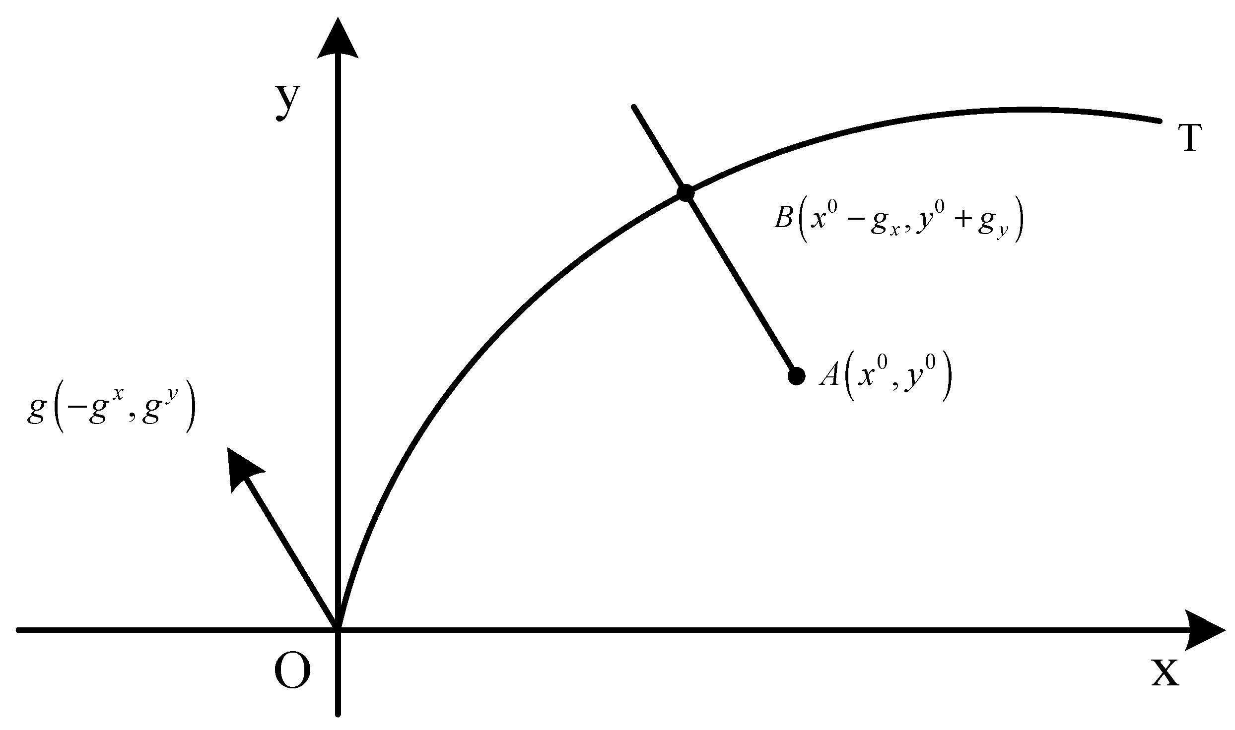
3.2.1. Traditional Directional Distance Function

In the field of efficiency evaluation, the directional distance function is one of the most representative frontier models in the world. The directional distance function (DDF) is a model derived from the DEA model. The basic idea of the directional distance function used in this paper is to reduce the input or undesired output by setting a direction vector to simultaneously expand the desired output.
We assume that a production process uses N input vectors x = ( x 1 , x 2 , , x n ) R N + to produce M desirable outputs y = ( y 1 , y 2 , , y m ) R M + . The production possibility set T ( x ) can be expressed as follows:
T = { ( x , y ) , x   can   produce   y }
The production possibility set T ( x ) has three characteristics, namely closed, bounded, and convex. In addition, the production possibility set T ( x ) is assumed to satisfy the following assumptions:
(1)
Input and output are disposed of at will. For example: if ( x , y ) T and ( x , y ) ( x , y ) , then ( x , y ) T .
(2)
Without input, there is no output, that is for ( x , y ) T , if x = 0 , then y = 0 .
(3)
The nature of inputs and outputs at the zero point is also possible without production, that is ( 0 , 0 ) T .
Based on the shortage function of Luenberger (1992) [43], this method can increase the output on the path specified by the direction vector used in the research and reduce the input, that is, the directivity distance function. The definition is as follows:
D r ( x , y , g ) = max { β : ( x β g x , y + β g y ) T }
where g = ( g x , g y ) is the direction vector that represents the maximum expansion of the output in the g x direction and the maximum reduction of the input in the g y direction. In addition, the traditional radial DDF approach assumes that the solution of the linear program reduces the inputs (or undesirable outputs) and expands the outputs at the same rate, denoted as β in Equation (2). β * = max β is the maximum ability to achieve the desired output expansion and the undesired output reduction. This model takes both expected and undesired outcomes into account. However, specific calculations and analyses cannot be performed alone. Therefore, the concept of a directional distance function is introduced in this paper. A directional distance function combines a desired output with an undesired output.
As shown in Figure 1, point A is the production point of the actual decision-making unit, while g = ( g x , g y ) is the direction vector, where g y and g x are the expansion of the output along the positive direction and the expansion of the input along the negative direction, namely the reduction of the input, respectively. Point A moves along the direction of g to point B, that is, the closer to the production frontier, the higher the production efficiency we get at this point. Therefore, we can use β to represent the ineffective part of input and output, The bigger β is, the lower the efficiency of the input and output is. If β = 0 , then the production efficiency has been achieved. According to this definition, we can use 1 β to express the total factor productivity.
About the directional distance function, there are several features:
(1)
D r ( x , y , g ) 0 , ( x , y ) T . This indicates that in the production possibility set, the value of the directional distance function is non-negative, and when ( x , y ) is on the production frontier, the value is equal to zero.
(2)
If ( x , y ) ( x , y ) T , then D r ( x , y , g ) D r ( x , y , g ) . This indicates that the value of the directional distance function will not increase if the output increases under the given input.
(3)
If ( x , y ) ( x , y ) T , then D r ( x , y , g ) D r ( x , y , g ) . This indicates that the value of the directional distance function will not decrease when the input increases under the given output.
(4)
D r ( x , y , g ) is a concave function.
In addition, the directional distance output function has the following conversion characteristics as shown in the following Equation (3):
D r ( x α g x , y + α g y , g ) = D r ( x , y , g ) α
It is obvious that the output y expands α g y , and x reduces α g x , which is equivalent to the value of the directional distance output function minus α .
The calculation of the optimal solution β can be solved using the non-parametric method data envelope analysis model. The solution for the mathematical programming is as follows:
D r ( x , y , g ) = max { β : ( x β g x , y + β g y ) T }
β * = max β s . t . { k = 1 K z k y m k ( 1 + β ) y 0 , m = 1 , , M k = 1 K z k x n k ( 1 β ) x 0 , n = 1 , , N z k 0 , k = 1 , , K
where k is the decision-making unit, that is, there are k = 1 , , K decision-making units.

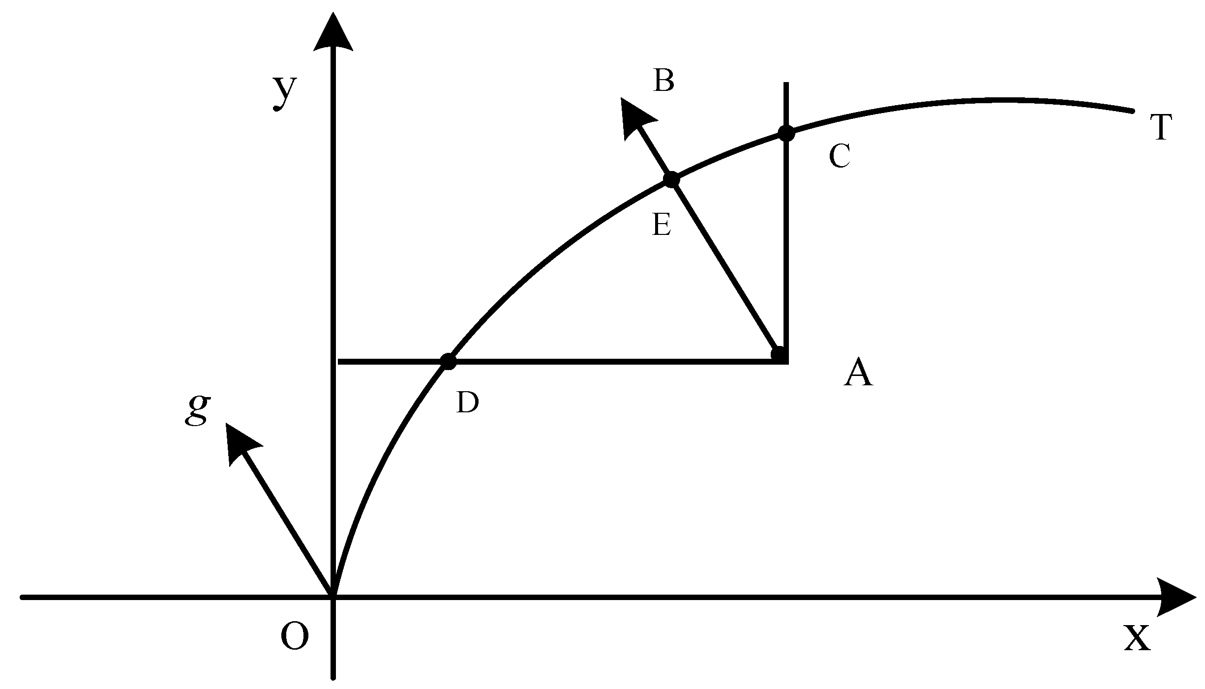
3.2.2. Non-Radial Directional Distance Function

The directional distance function assumes that the increase of output and the decrease of input are carried out in the same proportion according to a given direction, so it can be regarded as a radial efficiency evaluation method. From the point of view of an axiomatic method, the radial method of measuring efficiency is a popular method because it has some ideal mathematical characteristics. However, when there are non-zero slack variables, the efficiency values obtained using the radial method may be overestimated. Therefore, Zhouab et al. (2012) made a correction to the above model of the directional distance function. He stated that the above formula will overestimate the efficiency because the above method considers that the different inputs and outputs have equal impact on the total productivity by default. However, in fact, the impact of input and output factors is different for a company or industry [38].
The definition of the non-radial direction distance function is as follows:
D o ( x , y , g ) = max { w T β : ( x , y ) + g d i a g ( β ) T }
where w = ( w x , w y ) T refers to a standardized weight vector, which is related to the number of inputs and outputs. g = ( g x , g y ) represents a specifically set direction vector, which stipulates the direction of changes in input and output. β = ( β x , β y ) T is the proportion of changes in input reduction and output increase.
The solution of the corresponding optimal solution is also the application of the data envelope analysis model, and its mathematical programming is expressed as follows:
D O ( x , y , g ) = max w x β x + w y β y
s . t . { k = 1 K z k y m k ( 1 + β y g y ) y 0 , m = 1 , , M k = 1 K z k x n k ( 1 β x g x ) x 0 , n = 1 , , N z k 0 , k = 1 , , K , β x , β y 0
In order to better explain the difference between the non-radial distance function and the traditional radial direction distance function, a simple schematic diagram is drawn, as shown in Figure 2.
In Figure 2, for the point A, if the traditional directional distance function is used according to the direction g , then the reference point on the frontier is obtained as point B. If the non-radial direction distance function is used, the reference point obtained may be any point on the DEC section. It can be seen clearly that the non-radial direction distance function is more general and flexible than the traditional direction distance function in the efficiency evaluation.

3.3. Global Malmquist Index Analysis

The global Malmquist index model is a Malmquist index calculation method proposed by Pastor and Lovell (2005) [44]. Taking the sum of all periods as a reference set, that is, the standard reference set for each period is:
S g = S 1 S 2 S p = { ( x j 1 , y j 1 ) } { ( x j 2 , y j 2 ) } { ( x j n , y j n ) }
Since each period refers to the same frontier, the calculated result is also a single Malmquist index:
M g ( x t + 1 , y t + 1 , x t , y t ) = E g ( x t + 1 , y t + 1 ) E g ( x t , y t )
Although the next period refers to the same global frontier when calculating the Malmquist index, the calculation of efficiency changes still uses their respective leading edges:
E C = E t + 1 ( x t + 1 , y t + 1 ) E t ( x t , y t )
The degree of the frontier t + 1 close to the global frontier can be represented using E g ( x t + 1 , y t + 1 ) E t + 1 ( x t + 1 , y t + 1 ) . The larger the ratio is, the closer the frontier t + 1 is to the global frontier. The degree of the frontier t close to the worldwide frontier can be represented using E g ( x t , y t ) E t ( x t , y t ) . The larger the ratio is, the closer the frontier t is to the global frontier. Compared with the frontier t , the variation of the frontier t + 1 can be represented using the ratio of two ratios:
T C g = E g ( x t + 1 , y t + 1 ) / E t + 1 ( x t + 1 , y t + 1 ) E g ( x t , y t ) / E t ( x t , y t ) = E g ( x t + 1 , y t + 1 ) E t + 1 ( x t + 1 , y t + 1 ) E t ( x t , y t ) E g ( x t , y t )
The Malmquist index can be decomposed into efficiency changes and technological changes:
M g ( x t + 1 , y t + 1 , x t , y t ) = E g ( x t + 1 , y t + 1 ) E g ( x t , y t ) = E t + 1 ( x t + 1 , y t + 1 ) E t ( x t , y t ) ( E g ( x t + 1 , y t + 1 ) E t + 1 ( x t + 1 , y t + 1 ) E t ( x t , y t ) E g ( x t , y t ) ) = E C × T C g
Since the evaluated “DMU (Decision-Making Unit)” is included in the global reference set, there is no feasible solution to the VRS (Variable Returns to Scale) model in the Global Malmquist index:
M g ( 2 , 1 ) × M g ( 3 , 2 ) = M g ( 3 , 1 )

4. Empirical Analysis

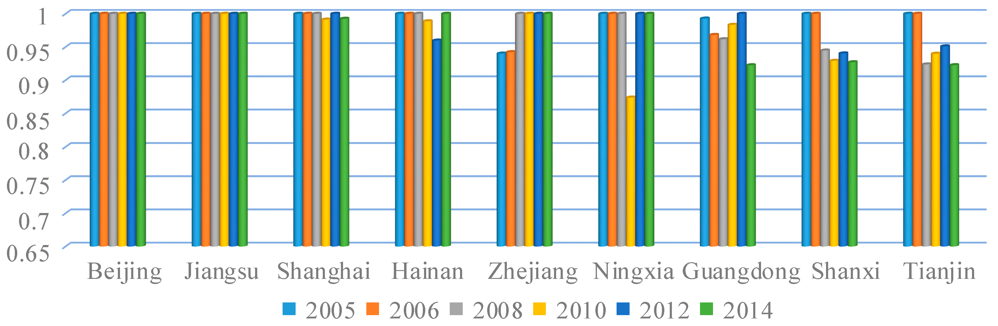
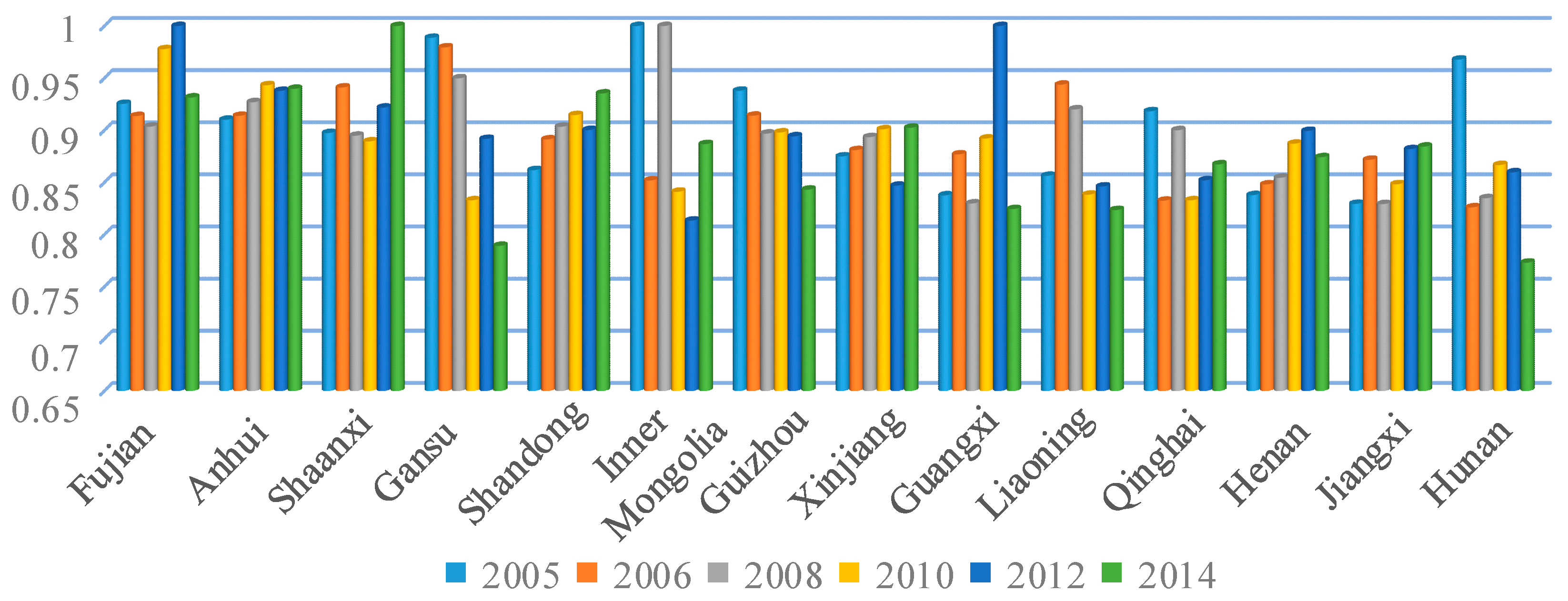
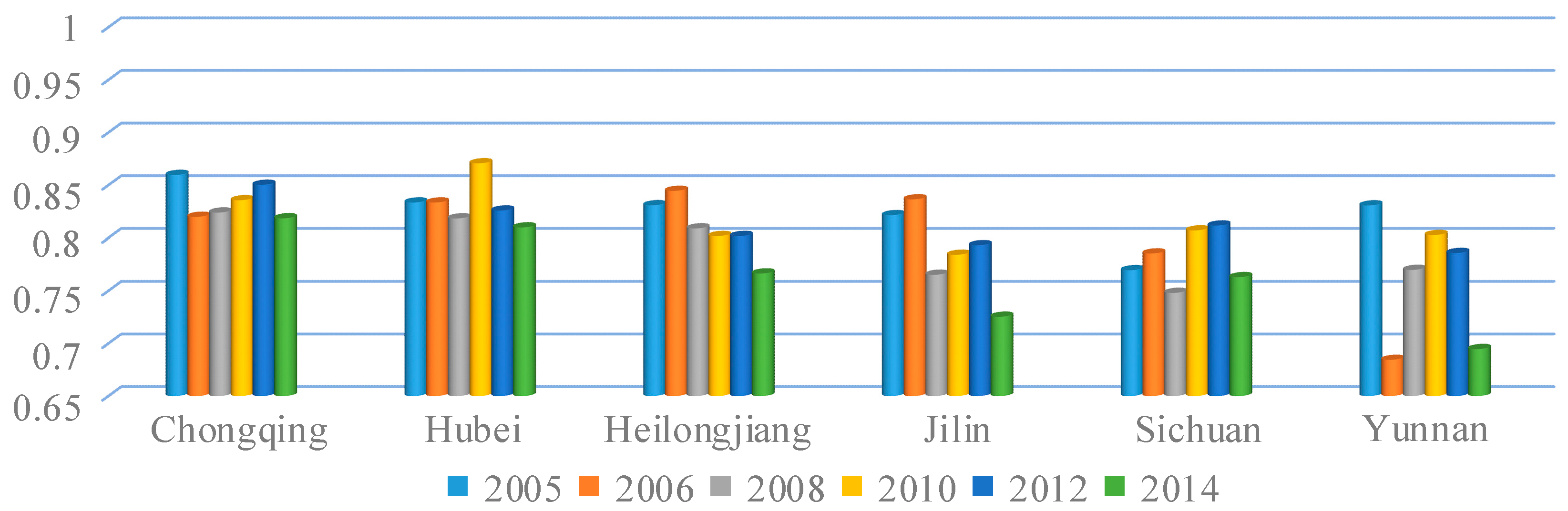
4.1. Static Result in Power System Productivity Efficiency

Through empirical study, we first calculated the static productivity efficiency for each province based on non-radial directional distance function, which considered carbon emissions as an undesirable output. Table 1 presented the result from 2005 to 2014 and the average productivity efficiency for each province. Also, we separated the results according to high efficiency (average productivity over 0.95), middle efficiency (average productivity over 0.85), and low efficiency group (all the rest) through Figure 3, Figure 4 and Figure 5, to present the distribution of power system productivity efficiency in China.
As the results shows, most high efficiency provinces during the entire observe period are located in the coastal area of China. At the same time, the largest efficiency group in China (14 provinces in total 30) have regional power system productivity efficiencies around 0.85 to 0.95, but most of these region’s power system productivity efficiency has been increasing during the last two years. While checking the low productivity efficiency group, it is clear that the mid-west area (include Chongqing, Hubei, Sichuan, and Yunnan), and the northeast part of China (Heilongjiang and Jilin, two out of three northeast provinces) were the less efficient part through the evaluation. These areas have also been treated as less developed areas in China.
Although the static results based on the non-radial directional distance function gave a general view of China’s region power system efficiency, are such results robust throughout a dynamic process?

4.2. Dynamic Efficiency Measurement

The global Malmquist index is a dynamic measurement method that can more effectively reflect the change of the maximum possible relative position between each decision-making unit and production boundary (efficiency change) and the movement of production boundaries (technology change). Table 2 shows the global Malmquist index of productivity efficiency of Chinese power systems for the period from 2005 to 2014.
First, we analyzed the global Malmquist index of productivity efficiency of Chinese power systems in 30 provinces during the same period. In 2014, it was found that the global Malmquist index of productivity efficiency of power systems in China’s economic developed provinces (Beijing, Tianjin, Jiangsu, Zhejiang, etc.) was generally high, while the t index of productivity efficiency of power systems in China’s undeveloped provinces (Shanxi, Mongolia, Guangxi, Shaanxi, Xinjiang, etc.) was generally low. In Mongolia, for example, although Mongolia’s efficiency change was high (up to 1), the global Malmquist index of productivity efficiency of power systems in Mongolia was still not high (only 0.624481). The reason is that the technical level in Mongolia is limited, resulting in low technological change (only 0.624481), which affected the global Malmquist index of productivity efficiency of power systems in Mongolia (only 0.624481). In contrast, the global Malmquist index of productivity efficiency of power systems was significantly higher due to the improvement of the technical level (technology change exceeding 1) in Gansu, Jiangxi, and Hebei.
From the perspective of efficiency change, in Guizhou, for example, the efficiency change was 1.002156, which shows that the efficiency of the thermal power system in Guizhou had dramatically improved. Meanwhile, compared with other provinces, due to the low improvement of the technical level (technology change was only 0.995762), the global Malmquist index of emission efficiency of power systems in Guizhou was significantly affected (only 0.997909). In contrast, due to high technology change and efficiency change, the global Malmquist index of emission efficiency of power systems in Yunnan and Guangdong was higher.
From the perspective of a different period in the same region, it was found that the improvement of production efficiency was mainly due to the development of the technical level. At the same time, to some extent, it was also affected by the efficiency improvement. In Yunnan, for example, although there were slight fluctuations, the global Malmquist index of productivity efficiency of power systems gradually rose from 2005 to 2014. In 2005, the Malmquist index was only 0.966891, but by 2014, it had reached 1.006. In this process, it is clear that the improvement of the global Malmquist index of emission efficiency of power systems resulted in the growth of efficiency change and technology change.
It can be concluded that the improvement of production efficiency was mainly due to the increase in technological change. Since 2005, China has paid more attention to environmental protection and has begun to improve the level of environmental protection technology and energy efficiency, which has brought about an improvement of the technical level.

4.3. Impact via Production Efficiency of Regional Thermal Power Systems to Regional Ecological Regulation Intensity

The correlation analysis in this section is based on panel data from the provinces in the mainland of China, with a time span of 2005–2014. The description of variables is as follows:
Stringency is the environmental regulation index, used as the core explained variable. Regarding the choice of environmental regulation index, it is still controversial because it cannot be directly quantified. The two major types of algorithm are the ones based on the measurement of pollution control inputs [45,46,47] and the one based on the measurement of pollution emissions [48]. This study followed the first path, establishing its environmental regulation stringency index as follows:
s t r i n g e n c y = A c t u a l   i n v e s t m e n t   i n   p o l l u t i o n   c o n t r o l i n d u s t r i a l   o u t p u t   v a l u e
Malm, EFF, and TECH are explained variables based on Section 4.2’s analysis. Malm is the global Malmquist index, which can more effectively reflect efficiency change and technology change. EFF is an efficiency change that indicates the evolution of the maximum possible relative position. TECH is a technology change that reflects each decision-making unit and production boundary.
Three control variables (Pub, Industry, Unemp) are added in the robustness test to analyze the correlation between environmental regulation intensity and the production efficiency of regional thermal power systems in 30 provinces. Among them, Pub is the proportion of fiscal expenditure in GDP, which reflects the government’s investment in power generation. Industry is the proportion of third industry GDP in total GDP, which reflects the industrial structure. Unemp is the unemployment rate, which reflects economic vitality. Table 3 gives the descriptive statistics for all data.
Then, we made a maximum likelihood regression and utilized the fix effect model and the random effect model to make a regression on Malm, EFF, and TECH. In the specific operation, a stepwise regression method was adopted, and 300 data points were randomly selected from the provinces of the country as sample sizes.
Meterage regression results for Malm and EFF are shown in Table 4 and Table 5. From both tables, it can be seen that when the impact of the Malmquist index and efficiency change on environmental regulation was tested separately, the adverse effect was not significant through testing; that is, the Malmquist index or the efficency change cannot directly affect environmental regulation. Control variables—Pub, Industry, and Unemp—were added in turn to analyze the influence by both index (Malmquist Index and Efficency change index). It can be observed that fiscal expenditure and third industry GDP had a direct negative effect on both indexes. The decrease in fiscal spending and third industry GDP had a negative impact on both indexes. Meanwhile the increase in the unemployment rate had a negative effect on both indexes.
It is shown in Table 6 that technology change had a significant adverse effect on stringency through hypothesis testing; that is, technology change directly affected environmental regulation. Control variables—Pub, Industry, and Unemp—were added in turn to examine the correlation between fiscal expenditure, third industry GDP, unemployment rate, and technology change. The results show that the decrease in fiscal expenditure and third industry GDP had a negative effect on technology change. While the increase in the unemployment rate had a negative effect on technology change.
By analyzing the results of meterage regression, it can be concluded that the technology change of production efficiency for China’s regional thermal power systems was the only factor that could directly decrease China’s regional environment stringency. Also, all of the control variables we selected had a significant impact on technology change. Among them, fiscal expenditure and third industry GDP had a negative effect on technology change because the government’s financial investment and third industrial spending effectively improved the level of technology, driving technological change. While the increase in the unemployment rate had a negative effect on technology change because the increase in unemployment reflected the lack of vitality in the economy, in which case, it was difficult to improve the technical level.

5. Conclusions and Recommendations

Using a non-radial directional distance function based on the DEA method, this study calculated the static electricity production efficiency of 30 Chinese provinces. Through the analysis of the global Malmquist index, the study further investigated the dynamic production efficiency of Chinese power systems. It was found that the main factor affecting the dynamic production efficiency was technological change. After the efficiency evaluation, an econometric analysis was conducted to investigate the relationship between environment stringency and the production efficiency of China’s regional thermal power systems. Based on empirical study results, we offer the following suggestions for improving the efficiency of China’s power system.
First, as provinces that had relatively high power production efficiencies, Jiangsu, Zhejiang, Shanghai, Beijing, and Tianjin had a higher degree of economic development. These cities and provinces were all well-known as being part of the “coastal developed area” of China. These areas already had fully exploited their advantages regarding resources and thermal industry construction. As empirical results show, the production efficiency for the thermal industry in these places had already reached their frontier. Therefore, these regions should start to transform their energy consumption and economic development to the renewable energy-based path faster than other regions of China.
Second, for provinces such as Inner Mongolia and Shanxi, the most coal-rich areas in China, the local government should consider quickly helping the region get rid of the development path of resource dependence. Although empirical results from this study may show the efficiency of thermal power production technology far exceeding the national average, it should be noted that this efficiency change only occurred in the short observation interval. However, this technical efficiency improvement was only based on the technological transformation of these provinces in the relevant year. Although the engineering transformation had improved the local thermal power production efficiency, it also brought the fact that the undertaking transformation cannot be quickly depreciated in the short term. Hence, such areas should further push their production efficiency to the efficiency frontier and accelerate the pursuit of technical efficiency to reduce the local environmental burden. At the same time, this type of region also needs to actively explore the development path of the service industry and upgrade the local industrial structure to achieve sustainable development.
Third, for provinces that are nearby areas with high power production efficiencies (e.g., Anhui, Jiangxi, and Hebei), radiation effects brought about by developed neighboring regions should be actively utilized. These less efficient provinces should rely on the industrial structure transformation of the developed coastal areas and absorb their transforming industries. Based on the transfer of these industries, the thermal power utilization efficiency for less efficient provinces will be further improved to optimize the overall thermal power production efficiency in the province to achieve further development of the region.
Finally, the central government should further focus on policy adjustment at the national level. For example, China’s central government should establish an effective multilateral exchange mechanism to promote the exchange of technology, expertise, and resources between regions with high power production efficiencies to surrounding regions, and throughout the country, to achieve sustainable development. Also, as technology has been demonstrated as the primary factor that can improve the power industries’ production efficiency, the contribution of technological advancements leading to a transition to a low-carbon power sector in China should be further exploited. The power industry must continue to show technological progress, acquire expert foreign personnel, and decommission small thermal power units with high rates of energy consumption and pollution, while simultaneous investing in coal-fired units with high efficiency and low carbon emissions. At the same time, further consideration should be given by China. For example, the central government should distinguish the technical efficiency of energy production in different regions, use both incentive and regulation policies to improve the power production efficiency for all regions, so the country can finally reach a balanced and sustainable future development.

Author Contributions

Z.P. and D.Z. conceived and designed the experiments; J.Z. performed the experiments; H.S. and J.Z. analyzed the data; Z.P. contributed analysis tools; Z.P. and J.Z. wrote the paper.

Funding

This research is supported by the China Social Science Fund (fund number 15CJL048), National Natural Science Foundation of China (fund number 71573121, 71774071), Jiangsu Social Science Fund (fund number 17ZTA001) and the Fundamental Research Funds for the Central Universities (fund number 3214007103).

Conflicts of Interest

The authors declare no conflict of interest.

References

  1. China Energy Statistical Yearbook 2015; China Statistic Press: Beijing, China, 2015.
  2. Statistical Bulletin of National Economic and Social Development of the P. R. China 2017. China Stat. 2018, 3, 7–20. (In Chinese)
  3. Chai, Q.; Zhang, X. Technologies and policies for the transition to a sustainable energy system in China. Energy 2010, 35, 3995–4002. [Google Scholar] [CrossRef]
  4. Nikolovski, S.; Reza Baghaee, H.; Mlakić, D. Anfis-based peak power shaving/curtailment in microgrids including pv units and besss. Energies 2018, 11, 2953. [Google Scholar] [CrossRef]
  5. Baghaee, H.R.; Mirsalim, M.; Gharehpetian, G.B.; Talebi, H.A. Reliability/cost-based multi-objective pareto optimal design of stand-alone wind/pv/fc generation microgrid system. Energy 2016, 115, 1022–1041. [Google Scholar] [CrossRef]
  6. Baghaee, H.R.; Mirsalim, M.; Gharehpetian, G.B.; Talebi, H.A. Decentralized sliding mode control of wg/pv/fc microgrids under unbalanced and nonlinear load conditions for on- and off-grid modes. IEEE Syst. J. 2017, 12, 3108–3119. [Google Scholar] [CrossRef]
  7. Baghaee, H.R.; Mirsalim, M.; Gharehpetian, G.B.; Talebi, H.A. A decentralized power management and sliding mode control strategy for hybrid AC/DC microgrids including renewable energy resources. IEEE Trans. Ind. Inform. 2017. [Google Scholar] [CrossRef]
  8. Baghaee, H.R.; Mirsalim, M.; Gharehpetian, G.B. Multi-objective optimal power management and sizing of a reliable wind/PV microgrid with hydrogen energy storage using MOPSO. J. Intel. Fuzzy Syst. 2017, 32, 1753–1773. [Google Scholar] [CrossRef]
  9. Lund, H.; Afgan, H.; Bogdan, Z. Renewable energy strategies for sustainable development. Energy 2007, 32, 912–919. [Google Scholar] [CrossRef] [Green Version]
  10. Kaygusuz, K.; Kaygusuz, A. Renewable energy and sustainable development in Turkey. Renew. Energy 2014, 25, 431–453. [Google Scholar] [CrossRef]
  11. Jiang, B.; Sun, Z.Q.; Liu, M.Q. China’s energy development strategy under the low-carbon economy. Energy 2010, 35, 4257–4264. [Google Scholar] [CrossRef]
  12. Zhang, Z.X. China in the transition to a low-carbon economy. Energy Policy 2010, 38, 6638–6653. [Google Scholar] [CrossRef] [Green Version]
  13. Hou, J.; Zhang, P.; Tian, Y.; Yuan, X.; Yang, Y. Developing low-carbon economy: Actions, challenges and solutions for energy savings in China. Renew. Energy 2011, 36, 3037–3042. [Google Scholar] [CrossRef] [Green Version]
  14. Zhang, N.; Lior, N.; Jin, H. The energy situation and its sustainable development strategy in China. Energy 2011, 36, 3639–3649. [Google Scholar] [CrossRef]
  15. Martin, N.; Worrell, E.; Schipper, L.; Blok, K. International Comparisons of Energy Efficiency, Workshop Proc; Utrecht University: Berkeley, CA, USA, 1994. [Google Scholar]
  16. Bagdadioglu, N.; Price, C.M.W.; Weyman-Jones, T.G. Efficiency and ownership in electricity distribution: A non-parametric model of the Turkish experience. Energy Econ. 1996, 18, 1–23. [Google Scholar] [CrossRef]
  17. Pollitt, M.G. Ownership and Efficiency in Nuclear Power Production. Oxford Econ. Pap. 1996, 48, 342–360. [Google Scholar] [CrossRef]
  18. Nagesha, N. Role of energy efficiency in sustainable development of small-scale industry clusters: An empirical study. Energy Sustain. Dev. 2008, 12, 34–39. [Google Scholar] [CrossRef]
  19. Cui, Q.; Li, Y. An empirical study on energy efficiency improving capacity: The case of fifteen countries. Energy Effic. 2015, 8, 1049–1062. [Google Scholar] [CrossRef]
  20. Mielnik, O.; Goldemberg, J. Communication The evolution of the “carbonization index” in developing countries. Energy Policy 1999, 27, 307–308. [Google Scholar] [CrossRef]
  21. Ang, B.W. Is the energy intensity a less useful indicator than the carbon factor in the study of climate change? Energy Policy 1999, 27, 943–946. [Google Scholar] [CrossRef]
  22. Soytas, U.; Sari, R.; Ewing, B.T. Energy consumption, income, and carbon emissions in the United States. Ecol. Econ. 2007, 62, 482–489. [Google Scholar] [CrossRef]
  23. Yuan, J.; Hu, Z.; Hu, Z. Cointegration and co-feature analysis on electricity consumption and economic growth in China. In Proceedings of the WSEAS International Conference on Applied Computer Science Canary Islands, Tenerife, Spain, 16–18 December 2006; pp. 347–351. [Google Scholar]
  24. Zeng, M.; Ma, X.C.; Yang, L.L. Design and analysis of adjustable carbon emissions allocation mechanism in electricity market. Power Syst. Technol. 2010, 34, 141–145. [Google Scholar]
  25. Zhao, X.; Ma, Q.; Yang, R. Factors Influencing CO2 Emissions in China’s Power Industry: Co-integration Analysis. Energy Policy 2013, 57, 89–98. [Google Scholar] [CrossRef]
  26. Chu, J.; Zeng, M.; Yang, L. Carbon Emissions Trading and Sustainable Development of Power Industry. In Proceedings of the International Conference on Electrical and Control Engineering, Wuhan, China, 25–27 June 2010; pp. 3443–3446. [Google Scholar]
  27. Yang, L.; Lin, B. Carbon dioxide-emission in China’s power industry: Evidence and policy implications. Renew. Sustain. Energy Rev. 2016, 60, 258–267. [Google Scholar] [CrossRef]
  28. Yan, D.; Lei, Y.; Li, L.; Song, W. Carbon emission efficiency and spatial clustering analyses in China’s thermal power industry: Evidence from the provincial level. J. Clean. Prod. 2017, 156, 518–527. [Google Scholar] [CrossRef]
  29. Li, M.J.; Tao, W.Q. Review of methodologies and polices for evaluation of energy efficiency in high energy-consuming industry. Appl. Energy 2017, 187, 203–215. [Google Scholar] [CrossRef]
  30. Yang, Q.; Wan, X.; Ma, H. Assessing Green Development Efficiency of Municipalities and Provinces in China Integrating Models of Super-Efficiency DEA and Malmquist Index. Sustainability 2015, 7, 4492–4510. [Google Scholar] [CrossRef] [Green Version]
  31. Huang, M.; Wang, B. Evaluating green performance of building products based on gray relational analysis and analytic hierarchy process. Environ. Progress Sustain. Energy 2015, 33, 1389–1395. [Google Scholar] [CrossRef]
  32. Bernard, J.T.; Côté, B. The measurement of the energy intensity of manufacturing industries: A principal components analysis. Energy Policy 2005, 33, 221–233. [Google Scholar] [CrossRef]
  33. Shang, L.; Wang, S. Application of Improved Principal Component Analysis in Comprehensive Assessment on Thermal Power Generation Units. Power Syst. Technol. 2014, 38, 1928–1933. [Google Scholar]
  34. Fan, Z.; Song, C.X.; Li, M.J. Study on Energy Efficiency Evaluation Index System for Fossil-fuel Power Plant. Energy Procedia 2014, 61, 1093–1098. [Google Scholar] [Green Version]
  35. Liang, J.; Long, S. Unified efficiency evaluation of regional industries in China: A nonradial directional distance function approach. Appl. Econ. Lett. 2017, 24, 1154–1160. [Google Scholar] [CrossRef]
  36. Xie, H.L.; Wang, W. Exploring the Spatial-Temporal Disparities of Urban Land Use Economic Efficiency in China and Its Influencing Factors under Environmental Constraints Based on a Sequential, Slacks-Based Model. Sustainability 2015, 7, 10171–10190. [Google Scholar] [CrossRef]
  37. Chung, Y.H.; Färe, R.; Grosskopf, S. Productivity and Undesirable Outputs: A Directional Distance Function Approach. Microeconomics 1997, 51, 229–240. [Google Scholar] [CrossRef]
  38. Zhou, P.; Wang, H. Energy and CO emission performance in electricity generation: A non-radial directional distance function approach. Eur. J. Oper. Res. 2012, 221, 625–635. [Google Scholar] [CrossRef]
  39. Wang, H.; Zhou, P.; Zhou, D.Q. Scenario-based energy efficiency and productivity in China: A non-radial directional distance function analysis. Energy Econ. 2013, 40, 795–803. [Google Scholar] [CrossRef]
  40. Wang, S.; Chu, C.; Chen, G. Efficiency and reduction cost of carbon emissions in China: A non-radial directional distance function method. J. Clean. Prod. 2016, 113, 624–634. [Google Scholar] [CrossRef]
  41. Wang, W.; Xie, H.; Lu, F. Measuring the Performance of Industrial Green Development Using a Non-Radial Directional Distance Function Approach: A Case Study of Jiangxi Province in China. Sustainability 2017, 9, 1757. [Google Scholar] [CrossRef]
  42. Luenberger, D.G. Benefit functions and duality. J. Math. Econ. 1992, 21, 461–481. [Google Scholar] [CrossRef] [Green Version]
  43. China Electric Power Yearbook; China Statistic Press: Beijing, China, 2015.
  44. Pastor, J.T.; Lovell, C.A.K. A Global Malmquist productivity index. Econ. Lett. 2005, 88, 266–271. [Google Scholar] [CrossRef]
  45. Becker, R.A. Air pollution abatement costs under the clean air act: Evidence from the pace survey. J. Environ. Econ. Manag. 2005, 50, 144–169. [Google Scholar] [CrossRef]
  46. Cole, M.A.; Elliott, R.J. Do environmental regulations cost jobs? an industry-level analysis of the UK. J. Econ. Anal. Policy 2007, 7, 1668. [Google Scholar] [CrossRef]
  47. Levinson, A. Environmental regulations and manufacturers’ location choices: Evidence from the census of manufactures. J. Public Econ. 1996, 62, 5–29. [Google Scholar] [CrossRef]
  48. Xing, Y.; Kolstad, C.D. Do lax environmental regulations attract foreign investment? Environ. Resour. Econ. 2002, 21, 1–22. [Google Scholar] [CrossRef]
Figure 1. The directional distance function that achieves the increase or decrease of the maximum ratio of output and input.
Sustainability 11 00659 g001
Figure 2. The difference between the non-radial distance function and radial distance function.
Sustainability 11 00659 g002
Figure 3. High efficiency group.
Sustainability 11 00659 g003
Figure 4. Middle efficiency group.
Sustainability 11 00659 g004
Figure 5. Low efficiency group.
Sustainability 11 00659 g005
Table 1. Emission efficiency of Chinese power systems for the period 2005–2014.
Province200520062008201020122014Average Productivity Efficiency
Beijing1.0001.0001.0001.0001.0001.0001.000
Tianjin1.0001.0000.9240.9400.9510.9230.956
Hebei0.9520.9630.8581.0001.0000.9640.956
Shanxi1.0001.0000.9450.9290.9400.9270.957
Inner Mongolia1.0000.8521.0000.8410.8130.8870.899
Liaoning0.8560.9440.9200.8380.8460.8240.871
Jilin0.8210.8360.7650.7840.7930.7250.788
Heilongjiang0.8310.8450.8090.8020.8020.7660.809
Shanghai1.0001.0001.0000.9911.0000.9930.997
Jiangsu1.0001.0001.0001.0001.0001.0001.000
Zhejiang0.9400.9421.0001.0001.0001.0000.980
Anhui0.9100.9140.9270.9430.9380.9400.929
Fujian0.9250.9140.9040.9781.0000.9310.942
Jiangxi0.8290.8720.8290.8480.8820.8840.857
Shandong0.8620.8910.9030.9150.9000.9350.901
Henan0.8380.8480.8540.8870.8990.8740.867
Hubei0.8340.8330.8180.8710.8260.8100.832
Hunan0.9680.8260.8350.8670.8600.7730.855
Guangdong0.9930.9680.9620.9831.0000.9220.971
Guangxi0.8380.8770.8300.8921.0000.8240.877
Hainan1.0001.0001.0000.9890.9601.0000.991
Chongqing0.8600.8200.8240.8360.8500.8180.835
Sichuan0.7700.7850.7480.8070.8120.7630.781
Guizhou0.9380.9140.8970.8980.8940.8430.897
Yunnan0.8310.6840.7700.8030.7860.6950.761
Shaanxi0.8970.9410.8950.8890.9221.0000.924
Gansu0.9890.9790.9500.8330.8920.7890.905
Qinghai0.9180.8330.9000.8330.8520.8670.867
Ningxia1.0001.0001.0000.8741.0001.0000.979
Xinjiang0.8750.8810.8930.9010.8470.9020.883
Table 2. Global Malmquist index of emission efficiency of Chinese power systems for the period 2005–2014.
Province200520072009201120132014
Malmquist IndexEfficiency ChangeTech ChangeMalmquist IndexEfficiency ChangeTech ChangeMalmquist IndexEfficiency ChangeTech ChangeMalmquist IndexEfficiency ChangeTech ChangeMalmquist IndexEfficiency ChangeTech ChangeMalmquist IndexEfficiency ChangeTech Change
Beijing0.99816710.9981671.00759611.0075961.00120711.0012070.99963310.999633111111
Tianjin0.99497110.9949711.00031811.0003180.9990650.9946821.0044060.99427910.9942791.0068110.9981611.0086661.0009140.9970851.00384
Hebei0.99183310.9918330.993130.8631911.1505331.0244151.0359010.9889120.97538110.9753811.0327310.9830741.0505121.0089660.9992271.009747
Shanxi1.00189211.0018921.0057840.9288491.0828281.0089920.9750961.0347610.9867321.0772390.9159831.1262681.0906331.0326740.9083840.9000881.009216
Inner Mongolia0.9812091.2064230.8133210.9781751.4609360.6695540.9978360.2402184.1538840.29152115.7628480.0184940.4342141.2021720.3611910.62448110.624481
Liaoning0.9966741.0575990.9423941.0034210.8995281.1154980.9947340.9051821.0989330.9817361.0220890.960520.9997130.9741141.0262791.0078761.0144760.993494
Jilin0.9974161.0333680.9652090.9993840.9821571.017541.0146631.0227580.9920840.9918611.0138650.9782971.0055220.9888191.0168910.9960970.9944291.001677
Heilongjiang1.0022981.0470810.9572311.0026750.9978071.0048791.0048860.9983341.0065630.9933531.0132590.9803551.0252561.0134311.0116690.9867860.9848041.002013
Shanghai1.00164111.0016411.00158711.0015871.00356311.0035631.0000671.0016530.9984171.01034311.010343111
Jiangsu0.97872610.9787260.9912110.991211.04298411.042984111111111
Zhejiang0.991741.0148260.9772520.97484610.9748461.03230411.0323041.00487911.0048791.04115211.041152111
Anhui0.9986720.9608181.0393971.0001810.9872271.0131221.0008910.979811.0215151.0068571.0361720.9717091.0370240.9991961.0378580.9886350.994650.993952
Fujian1.0012461.0059670.9953071.000831.0009630.9998671.0108741.0256320.985610.995940.9950821.0008621.01190.9845561.0277730.9902460.9909540.999286
Jiangxi0.9997991.0229680.977350.9920530.9853531.00681.0008550.9987131.0021450.9986991.0075370.9912281.0055640.9999081.0056561.0010960.9995291.001568
Shandong0.9474250.9932750.953840.9911621.2606010.7862611.0079091.50.6719390.996871.1092270.8987061.2645031.1587961.0912210.9067880.9199490.985694
Henan0.9894261.2032530.8222930.9863160.9568741.0307691.0386521.0759280.9653550.9476571.0445820.9072111.0621910.8948011.1870690.9743970.9881760.986055
Hubei1.0022151.0287490.9742081.0016010.9984611.0031441.0075131.005191.0023111.0000671.0092530.9908991.0134691.0089791.004451.0025370.9917171.01091
Hunan1.015491.0718260.9474391.0014950.997451.0040551.0052361.0007691.0044640.9905050.9989650.9915311.0130231.0004781.0125390.9955330.9938991.001644
Guangdong0.98628410.9862841.04587711.0458771.03633911.0363390.99623210.9962321.0156950.9735031.043341.0333841.0272181.006002
Guangxi1.0007221.019080.9819850.9911790.989461.0017381.0033841.0002711.0031110.9948751.0039360.9909751.02769911.0276990.9766560.9776150.999019
Hainan1110.99953610.9995360.99973810.9997380.99901110.999011111111
Chongqing1.0003381.0145120.9860290.994780.9871551.0077241.0022871.001411.0008760.999711.0257510.9746131.0061241.0068380.9992910.9955160.9859551.009698
Sichuan0.9958991.0354670.9617871.0013221.003940.9973921.008091.0069861.0010960.9999991.0079630.9920991.0066680.9780271.0292840.9897650.9896211.000145
Guizhou0.99260610.9926060.9971890.9752291.0225170.9994681.0514190.950590.9886551.0105950.978291.0078320.9886151.0194390.9979091.0021560.995762
Yunnan0.9668910.9558081.0115961.0178161.0324390.9858361.0045751.0069240.9976670.9905251.0141650.976691.0128280.9976321.0152331.0060021.004161.001835
Shaanxi1.0006661.0158350.9850680.9950880.9606261.0358740.9950270.9787441.0166361.0068481.021160.9859851.0530781.029361.0230410.96943610.969436
Gansu0.9985140.9986210.9998920.9984130.9761091.022850.9958070.9828981.0131341.0056731.019250.986680.9933040.9836621.0098021.0008020.998631.002175
Qinghai1111.00060111.0006011.00163211.0016320.99602810.9960281.00586311.0058630.99519910.995199
Ningxia0.99843410.9984340.99878910.9987890.9975910.972561.0257371.0005731.0367980.965061111111
Xinjiang1.000981.0172750.9839820.9992020.9905861.0086980.9918760.9828241.009210.9895860.9982870.9912841.0077580.9917911.0160990.9869820.9896690.997286
Table 3. Descriptive statistical results.
VariableMeaningUnitNMeanMaxMinSD
StringencyEnvironment Regulation -30042.83353280.393.5934.60319
MalmMalmquist Index-3001.0049294.26710.29150.19878
EFFEffinecy Change-3001.04871215.76280.2402180.8571323
TECHTechnology Change-3001.0248464.8136930.0184940.3395874
PubFiscal expenditure/GDP%30020.7641361.217.988.9759
IndustryThird Industry GDP/GDP%30040.144577.9528.628.1988
UnempUnemployment rate%3003.60325.71.210.6477
Table 4. Panel Regression Result for Global Malmquist Index with Regional Environmental Regulation Strength.
Independent Variables123456789101112
Malm−10.33−10.2−10.27−9.87−10.41−9.78−9.78−9.59−10.33−10.2−10.27−9.87
(7.28)(7.37)(7.36)(7.25)(7.3)(7.19)(7.21)(7.17)(7.28)(7.37)(7.36)(7.25)
Pub −0.23−0.210.07 −1.2 ***−1.2 ***−0.71 −0.23−0.210.07
(0.32)(0.32)(0.33) (0.39)(0.4)(0.48) (0.32)(0.32)(0.33)
Industry −0.340.01 0.0040.09 −0.340.01
(0.38)(0.4) (0.52)(0.52) (0.38)(0.4)
Unemp 12.91 *** 10.95 * 12.91 ***
(4.52) (5.67) (4.52)
Constant53.22 ***58 ***71.54 ***4.0453.3 ***77.63 ***77.78 ***23.7453.22 ***58 ***71.54 ***4.04
(8.72)(10.72)(18.09)(29.8)(7.47)(10.74)(21.53)(35.23)(8.72)(10.72)(18.09)(29.8)
Fix EffectNNNNYYYYNNNN
Random EffectNNNNNNNNYYYY
R-square0.0030.02430.0020.02410.0030.06470.06460.00660.0030.02430.0020.0241
N300300300300300300300300300300300300
* p < 0.1, ** p < 0.05, *** p < 0.01.
Table 5. Panel Regression Result for Efficiency Change Index with Regional Environmental Regulation Strength.
Independent Variables123456789101112
EFF−0.57−0.54−0.58−0.49−0.63−0.53−0.529−0.469−0.57−0.54−0.58−0.49
(1.75)(1.77)(1.77)(1.74)(1.76)(1.73)(1.74)(1.72)(1.75)(1.77)(1.77)(1.74)
Pub −0.24−0.220.07 −1.22 ***−1.22 ***−0.72 −0.24−0.220.07
(0.32)(0.32)(0.34) (0.39)(0.4)(0.47) (0.32)(0.32)(0.34)
Industry −0.340.021 0.0010.1 −0.340.021
(0.38)(0.4) (0.52)(0.52) (0.38)(0.4)
Unemp 12.99 *** 11.02 * 12.99 ***
(4.52) (5.68) (4.52)
Constant43.43 ***48.38 ***61.87 ***−5.7943.49 ***68.62 ***68.58 ***14.2843.43 ***48.38 ***61.87 ***−5.79
(5.08)(8.09)(16.69)(28.96)(2.34)(8.34)(20.46)(34.61)(5.08)(8.09)(16.69)(28.96)
Fix EffectNNNNYYYYNNNN
Random EffectNNNNNNNNYYYY
R-square00.0690.00750.02100.0720.0720.009200.0690.00750.021
N300300300300300300300300300300300300
* p < 0.1, ** p < 0.05, *** p < 0.01.
Table 6. Panel Regression Result for Technology Change Index with Regional Environmental Regulation Strength.
Independent Variables123456789101112
TECH−7.85 *−7.71 *−7.7 *−7.77 *−8.28 *−8.01 *−8.01 *−8.03 *−7.84 *−7.71 *−7.7 *−7.77 *
(4.57)(4.62)(4.61)(4.54)(4.61)(4.54)(4.55)(4.52)(4.57)(4.62)(4.61)(4.54)
Pub −0.24−0.220.07 −1.2 ***−1.2 ***−0.7 −0.24−0.220.07
(0.32)(0.32)(0.33) (0.38)(0.4)(0.47) (0.32)(0.32)(0.33)
Industry −0.340.029 0.020.12 −0.340.029
(0.38)(0.4) (0.52)(0.51) (0.38)(0.4)
Unemp 13.05 *** 11.07 * 13.05 ***
(4.5) (5.6) (4.5)
Constant50.88 ***55.67 ***68.82 ***1.0351.32 ***76.05 ***75.33 ***20.8950.88 ***55.67 ***68.82 ***1.03
(6.66)(9.13)(17.1)(29.06)(4.94)(9.28)(20.65)(34.55)(6.66)(9.13)(17.1)(29.06)
Fix EffectNNNNYYYYNNNN
Random EffectNNNNNNNNYYYY
R-square0.00170.0190.00210.02350.00170.06280.06340.00640.00170.0190.00210.0235
N300300300300300300300300300300300300
* p < 0.1, ** p < 0.05, *** p < 0.01.

