Article

Simulation of Drainage Capacity in a Coastal Nuclear Power Plant under Extreme Rainfall and Tropical Storm

1
Guangdong Key Laboratory of Coastal Ocean Variability and Disaster Prediction, Guangdong Ocean University, Zhanjiang 524088, China
2
School of Resource and Environmental Science, Wuhan University, Wuhan 430072, China
*
Author to whom correspondence should be addressed.
Sustainability 2019, 11(3), 642; https://doi.org/10.3390/su11030642
Submission received: 29 November 2018 / Revised: 21 January 2019 / Accepted: 23 January 2019 / Published: 26 January 2019

Abstract

:
To ensure the safety of coastal nuclear power plants, accurately simulating water depth due to flooding resulting from heavy rainfall and tropical storms is important. In this paper, a combined model is developed to analyze and simulate the drainage capacity in a coastal nuclear power plant under the combined action of extreme rainfall and wave overtopping. The combined model consist of a surface two-dimensional flood-routing model, a pipe network model, and an offshore wave model. The method of predictive correction calculation is adopted to calculate the node return flow. The inundated water depth varying with time for different design rainstorm return periods (p = 0.1 and 1%) was simulated and analyzed by the combined model. The maximum inundated water depth is calculated for the important entrances of the workshop. The model was validated and calibrated with the data of the rainfall, outflow discharge, and flow velocity measured on 23 June 2016 in plant. Modeling indicates that the simulated depths are consistent with the observed depths. The results show that the water depths in the left and right of the nuclear power plant are 0.2–0.4 m and 0.3–0.8 m, respectively. The water depth increases of Monitoring Point 22 are the largest in different design rainstorm return periods (p = 0.1 and 1%), which increase by 16% for a rainstorm once every thousand years compared to events occurring once in one hundred years. The main factor influencing water accumulation is wave overtopping, and the seawall, revetments, and pipe system play an important role in decreasing the inundated water depth. Through scientific analysis, a certain decision-making basis has been provided for flood disaster management and a certain security guarantee has also been provided for regional sustainable development.

1. Introduction

Intense rainfall and tropical storms in coastal areas often generate flooding due to the limited capacity of drainage systems, especially for coastal nuclear power plants. The flood inundation can lead to large casualties and property losses [1,2,3]. The nuclear accidents triggered by the 2011 earthquake and the tsunami in Japan have raised concerns over the safety of nuclear power use. These concerns underscore both the importance of flood control systems for coastal nuclear plants and the influence of flood control design on the safety and efficiency of nuclear power plants [4,5]. Environmental security is a guarantee of sustainable development. Therefore, the prediction and assessment of flood risk is not only an important basis for regional flood risk management but also a universal need for regional disaster prevention and reduction and for sustainable development.
Numerical simulation is an important method used for predicting and assessing overland flooding and underground network drainage [6,7,8,9,10,11,12,13]. A number of combined models have been widely used to analyze inundation by flooding in recent years. Lin et al. integrated a two-dimensional (2D) model (depth-integrated velocities and solute transport (DIVAST)) with a one-dimensional (1D) flood and a channel model to enhance its ability to simulate floodplain flows; in the study, complex flow situations were considered [14]. Adeogun et al. estimated flood damage due to sewer overflow using a 1D storm-water management model (SWMM) with a 2D hydrodynamic model. The flow back into the sewer network from the surface during the recession limb of the hydrograph was not considered [15]. Son et al. employed a 1D–2D combined mathematical modeling technique to represent the effect of underground spaces on flood characteristics, including the flood depth, area, and velocity of urban overland floodwaters [16]. Xie et al. used an SWMM and a low-impact development (LID) model to contrast the rainfall regulation effect between permeable pavement and grassed swales [17]. Yazdi employed an SWMM–EPA (Environmental Protection Agency) simulation model and combination entropy theory to predict the time series of water quality parameters in selected pipes or channels of the network [18]. These studies effectively simulated urban surface runoff and flow within a drainage pipe network.
Many scholars have studied coastal floods caused by natural phenomena such as typhoons, tropical storms, and heavy rainfall [19,20,21,22]. For example, Chen et al. developed a combined model to simulate the flood process under the combined action of extreme rainfall, wave overtopping, and tidal flow in a coastal nuclear power plant [23]. Ren et al. employed a complex hydrological–hydraulic model that included the tide of the sea, slope runoff from the rain, a pipe flow, and urban channel flow to simulate municipal drainage and urban channel flooding in a coastal city [24]. Hsu et al. estimated extreme wave conditions and storm surges by numerical simulation using the wind wave model (WWM), the Princeton ocean model (POM), and the analytic hierarchy process (AHP) to establish a risk map of the study areas [25]. Lopes et al. assessed marine-induced inundation in coastal lagoons under extreme sea levels induced by astronomic tide and storm surge events. The approach employed integrated joint probability analysis of sea surface elevation (SSE) data to determine extreme sea levels for a given return period of storm surges [26]. Karim et al. used a calibrated numerical hydrodynamic model to simulate surge wave propagation through the rivers and overland flooding, and the study focused on the impacts of sea surface temperature (SST) rise and sea-level rise (SLR) in terms of intensified surge heights at the coast [27]. These studies indicate the importance of model coupling in flood calculation. Compared with the diversity of the combined calculation method for horizontal connection, the calculation method of vertical connection is not mature, which needs further research. At present, it mainly includes the weir flow formula method or the simplified weir flow formula method, the orifice outflow method, and so on. A new method for calculating vertical water flow exchange was proposed in the study, and a vertical connection between the 1D and 2D models was established. The method of predictive correction calculation was adopted to calculate the node return flow, and the result was more accurate.
In this study, the combined model includes a surface 2D flood-routing model, an offshore wave model, and a hydrodynamic model of a drainage pipe network. This model is used to simulate flooding inundation caused by wave overtopping and heavy rainfall at a coastal nuclear power plant. The different design rainstorm return periods (p = 0.1 and 1%) and the overtopping effect of high waves are considered. The maximum inundated water depth is calculated for different scenarios at important entrances to the workshop.

2. Mathematical Model

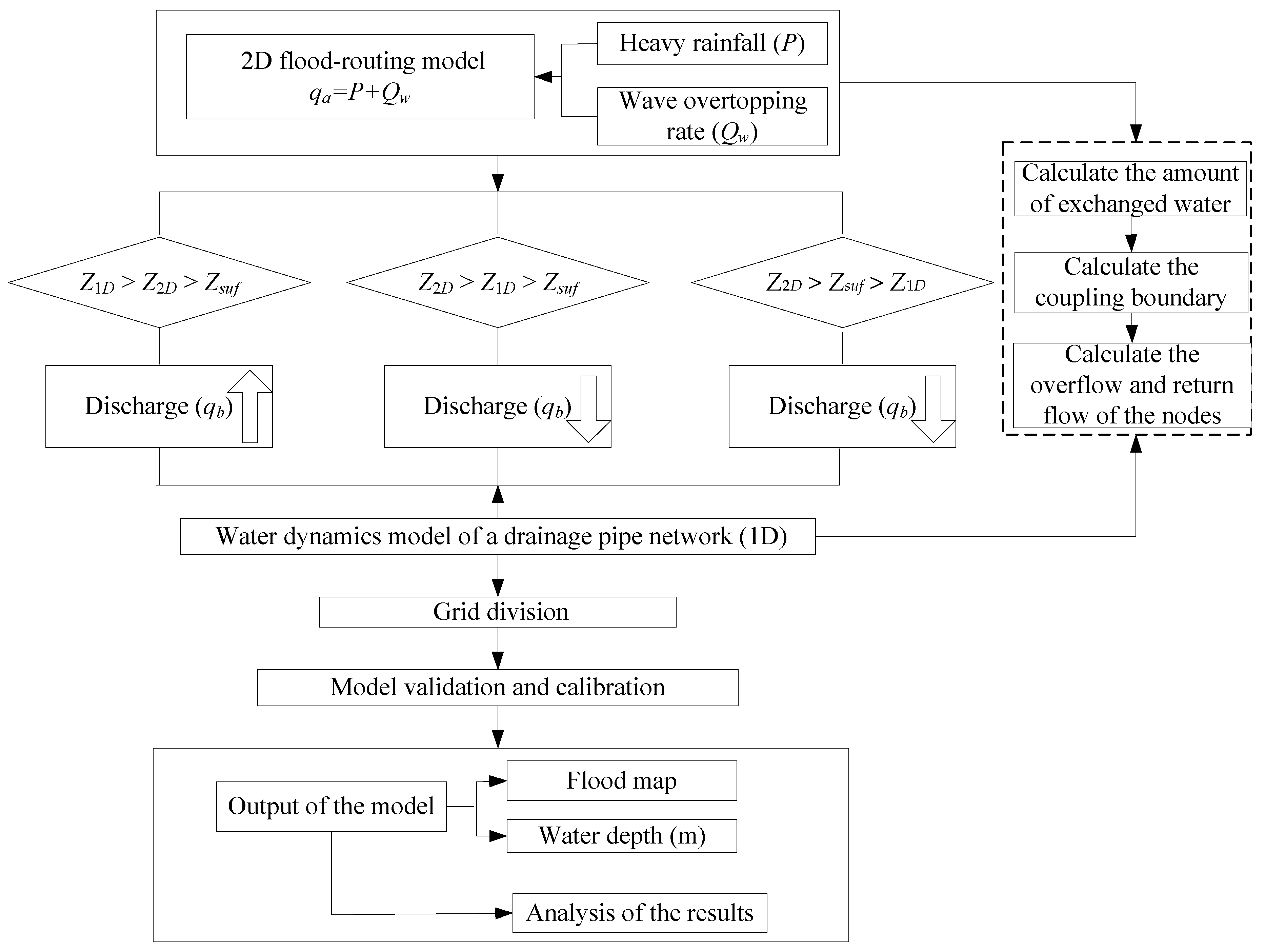
2.1. The 2D Flood-Routing Model

The continuity equation and the 2D shallow-water equation were incorporated in 2D Saint-Venant equations for overland flow. The equation under a rectangular coordinate system can be expressed as [28]
h t + ( h u ) x + ( h v ) y = q a q b .
The momentum equation for the x-axis can be written as
h u t + h u u x + h v u y + g h z x + g n 2 h u 2 + v 2 u h 4 3 = x ( h γ t u x ) + y ( h γ t u y ) .
The momentum equation for the y-axis can be written as
h v t + h u v x + h v v y + g h z y + g n 2 h u 2 + v 2 v h 4 3 = x ( h γ t v x ) + y ( h γ t v y )
where h is the water depth (m); u and v are the vertical average velocities (m/s) on the x- and y-axes, respectively; t is time (s); qa is the source term used to reflect precipitation and the wave overtopping rate; qb is the source term to reflect the discharge exchange between the surface flow and pipe flow; Z is the bottom elevation; n is the Manning roughness coefficient; γt is the turbulent viscosity coefficient (m2/s).

2.2. The Water Dynamics Model of a Drainage Pipe Network

The continuity equation and the one-dimensional Saint-Venant equation are adopted in SWMM for the flow through a drainage pipe network [23]:
A t + Q x = 0
where Q is the discharge in the pipe (m3/s), and A is the cross-sectional flow area (m2).
The momentum equation is
g A H P x + ( Q 2 / A ) x + Q t + g A S f + g A h L = 0
where HP is the water level in the pipe (m), Sf is the friction slope, and hL is the local resistance loss of the unit length, expressed as follows:
S f = K g A R 4 / 3 Q | V |
h L = K V 2 2 g L
where K = gn2, R is the hydraulic radius of the flow cross-section (m), V is the flow velocity (m/s), and L is the conduit length (m). The absolute value indicates that the direction of resistance from friction is opposite to the direction of the flow.
We only considered pressurized flows through the drainage structures and the drainage pipe, and the flow exchange was assumed to be influenced primarily by the head difference between the street and pipe flows. Thus, the simulation excluded the effects of transition from free surfaces to pressurized flow in the pipe.

2.3. Wave Overtopping Model

The offshore wave model (SWAN) was adopted to simulate the offshore wave near the nuclear power plant. In SWAN, the evolution of the wave spectrum is described by the spectral action balance equation, which is expressed by Cartesian coordinates as follows [29,30].
In the process of wave propagation to the front of the seawall at the site of the plant, the phenomena of refraction, diffraction, and reflection are caused by the blocking of the island and the change in local topography. Therefore, the BW model developed by the DHI (Danish Institute of Hydraulics) was used to calculate the wave elements in front of the embankment. This model is based on the improved Boussinesq equation [31,32].

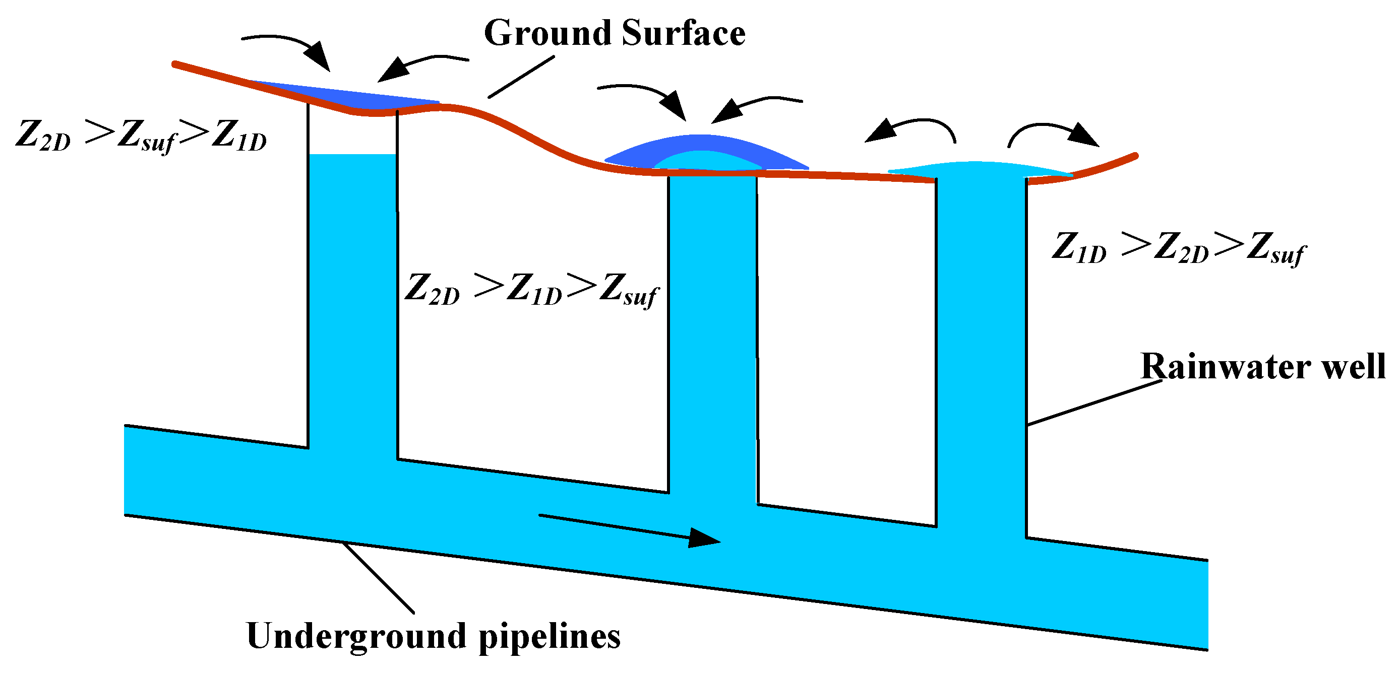
2.4. Coupling Calculation of Surface Runoff and Drainage Pipe Network Flow

The coupling of one- and two-dimensional models in the vertical direction—the surface and underground coupling of one- and two-dimensional models—mainly addresses the problems between the underground drainage network and surface runoff exchange. The exchange of flow is assumed to occur mainly through nodes (catch-basin, inspection wells, etc.), with the water level of the nodes set as Z1D, the water level of the surface runoff set as Z2D, and the level of the ground surface set as Zsuf (Figure 1). The water flow interaction of the 1D model and the 2D model in the vertical direction can be divided into the following two cases [33]:
(1) The Node Overflow
When the drainage capacity is insufficient, the water level of the drainage system in the 1D model is greater than the water level in the 2D model and, as a consequence, the ground surface level, i.e., Z1D > Z2D > Zsuf. In this case, the water flows from the pipe network to the surface, that is the node overflows. The key to model coupling is to calculate the amount of water flowing from the pipeline to the surface, that is, the amount of overflow.
Taking into account the current flow condition of the next time step of the pipe network, the method of fixing the node water level was used to calculate the overflow flow. The main steps are as follows:
(a) Assume that the node does not overflow, and calculate the water level of the node. At this time, the water balance of the node mainly considers the amount of water flowing into and out of each pipe segment and the change in the water volume of the node.
(b) Compare the node and surface water level. If the node water level is lower than the surface water level, the node does not overflow and terminates the calculation of the overflow. If the node water level is higher than the surface water level, the node is considered to be overflowing, and the node water level should be reset. Reset the node water level to be equal to the surface water level, that is Znod = Zsuf, and, based on this, calculate the flow rate of each pipe segment connected to the node.
(c) Calculate the amount of exchanged water. Assume that there are m pipes connected to the nodes and that the exchange flow of the nodes to the surface is Q n s . The exchange flow of the nodes to the surface can thus be
Q n s = i = 1 m Q i t A n o d ( Z n o d n + 1 Z n o d n ) t
where Anod is the water storage area of the node. Z n o d n + 1 and Z n o d n are the water level values of the current time step and the previous time step of the node, respectively. Qi is the flow rate of the ith pipe segment connected to the node, with positive inflow and negative outflow.
(2) The return Flow of the Node
The water level in the 1D model was lower than the water level in the 2D model, but greater than the ground surface level, i.e., Z2D > Z1D > Zsuf. The water level in the 1D model was lower than the ground surface level and, as a consequence, the 2D water level, i.e., Z2D > Zsuf > Z1D. In this case, the water flows from the surface to the pipe network, that is, the return flow of the node. The key to model coupling is to calculate the amount of water flowing from the surface to the node. The amount of return flow can be calculated according to different coefficients, such as the flow coefficient, the side contraction coefficient, the perimeter of the node, etc.
In this study, a predictive correction method was used to calculate the return flow. In this method, the weir flow formula is used to estimate the maximum possible backflow, and the model is calculated and iteratively solved. If the water level of the node is lower than the surface water level and no overflow occurs, no correction is needed. Otherwise, the flow rate is corrected according to the overflow flow.
(a) Estimate the return flow. According to the current time step, the water level difference between the surface and the node is used to estimate the maximum possible return flow using the weir flow formula, which can be shown as follows:
Q s n u n _ p r o = { m 1 ε C n o d h s u r 2 g h s u r i f h n o d h s u f 2 3 m 2 ε C n o d h n o d 2 g ( h s u r h n o d ) i f 2 3 < h n o d h s u f 1
where m1 and m2 are flow coefficients, varying from 0 to 1. ɛ is the side contraction coefficient. Q s n u n _ p r o is the unrestricted estimated node return traffic. hsur and hnod are the differences between the surface water level, the node water level, and the surface elevation, and Cnod is the perimeter of the node or the width of the rain.
In order to ensure the stability of the model, the following formula is used to limit the return flow:
Q s n p r o = m i n ( Q s n u n _ p r o , Q e m )
where Q s n p r o is the estimated node return traffic, and Q e m is the maximum allowed exchange flow.
(b) Calculate the amount of backflow correction. The estimated backflow is substituted into the node water level iteration process of the one-dimensional model, and the backflow is corrected according to the node overflow:
Q s n = { Q s n p r o i f Q n s c o r = 0 Q s n p r o Q n s c o r i f Q n s c o r > 0   a n d   Q n s c o r Q s n p r o
where Q s n p r o is the overflow amount that may occur, and Q s n is the corrected return flow amount.
(c) Substitute the corrected return flow amount as a source term into the two-dimensional model and update to the next time step.
It can be seen from the node overflow and the return flow calculation process that the vertical coupling of the model will update the one-dimensional model first, and the two-dimensional model a time step afterward. Whether it is an iterative solution of node overflow or a predictive correction calculation of node reflow, the solution method used in this paper was realized in the iterative solution process of node water level without additional iterative solution, which not only ensures the accuracy of the result but also keeps its model efficiency. The flowchart for the numerical scheme is shown in Figure 2.

3. Model Application

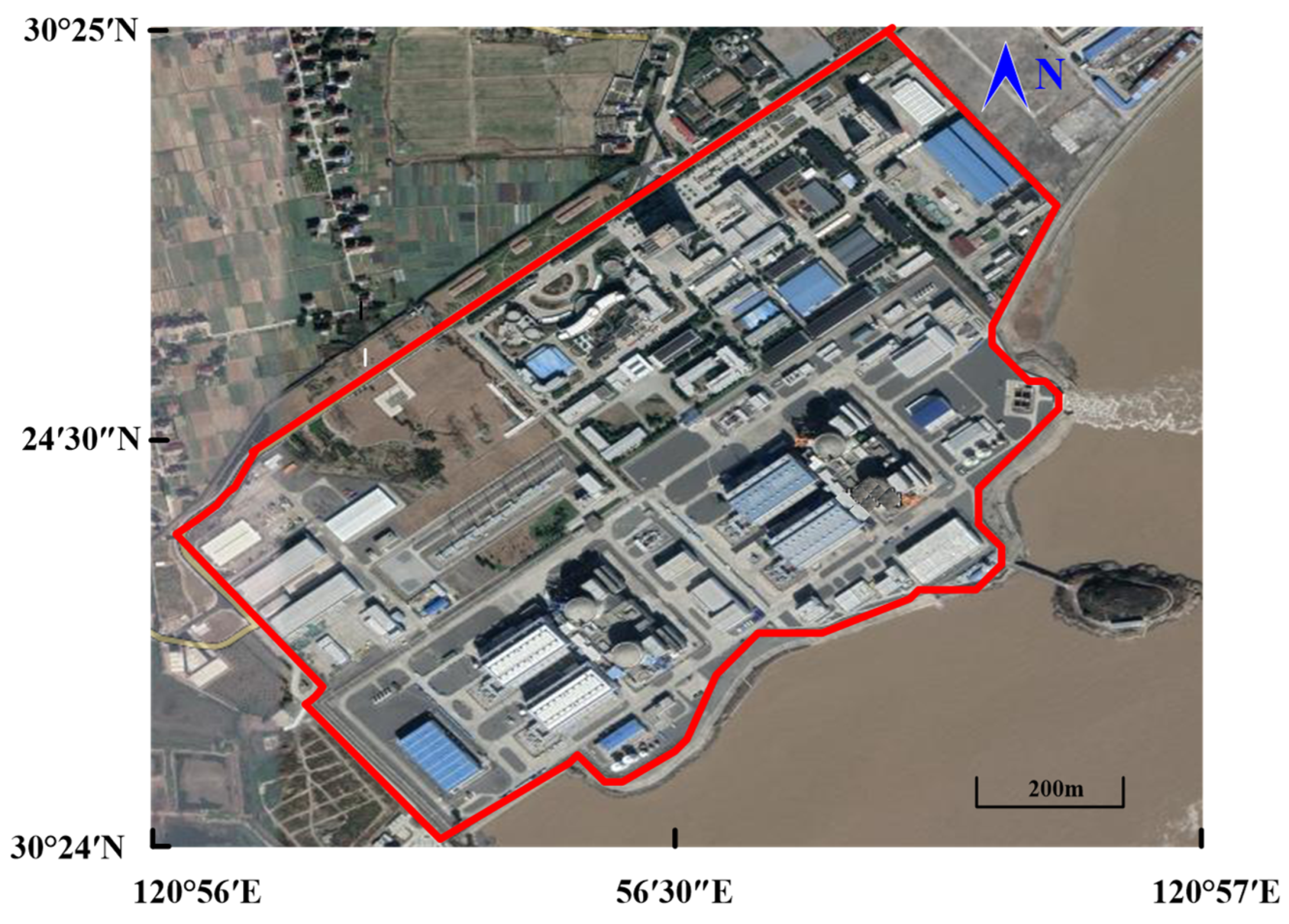
3.1. Description of Case Study Area

The nuclear power plant is close to the coast, and is extremely vulnerable to floods caused by typhoons and tropical storms. Its geographical position is shown in Figure 3. The site of the nuclear power plant is located on a mountain. Prior to the construction of the plant, the highest elevation of the plant was 83.2 m. Because the nuclear island of the nuclear power plant and other buildings need to be located on the bedrock so that the foundation has sufficient bearing capacity, the geological conditions determine the upper limit of the design plant elevation. According to the design flood and geological conditions of the nuclear power plant, the designed plant elevation of the nuclear power plant was set as 10.93 m. Based on the highest elevation of 83.2 m of the plant, a 72.27 m excavation was completed at the nuclear power plant. The eastern elevation of the nuclear power plant is lower than the other areas. The target area is not near to a river that can overflow its banks during a flood. According to the local exposure to storms, nuclear plants that face gulfs require an arc seawall 1.5 m high. Hence, the south and southeast flanks of the nuclear power plant are protected by a wave wall approximately 500 m from the plant site. As such, the wave wall can effectively reduce the foreshore and flow height. The elevation of the nuclear power plant is 10.93 m. The absolute elevation of the main technical workshop is 11.23 m.

3.2. Calculation Area and Grid Division

The grid, using the topographic map of the ground surface of the plant, was generated according to the size of the pipe network entrance, the pipe network segment, the catch-basin and pipeline node distribution, the surface elevation, and the building distribution in the plant area. This map was combined with the layout and elevation data of the nuclear power plant building using TECPLOT software (Tecplot 10.0, Tecplot Inc, Bellevue, WA, USA) to generalize the building. The model computing grid was generated, an irregular mesh was adopted, and local grid refinement was conducted based on the characteristics of the catch basin.

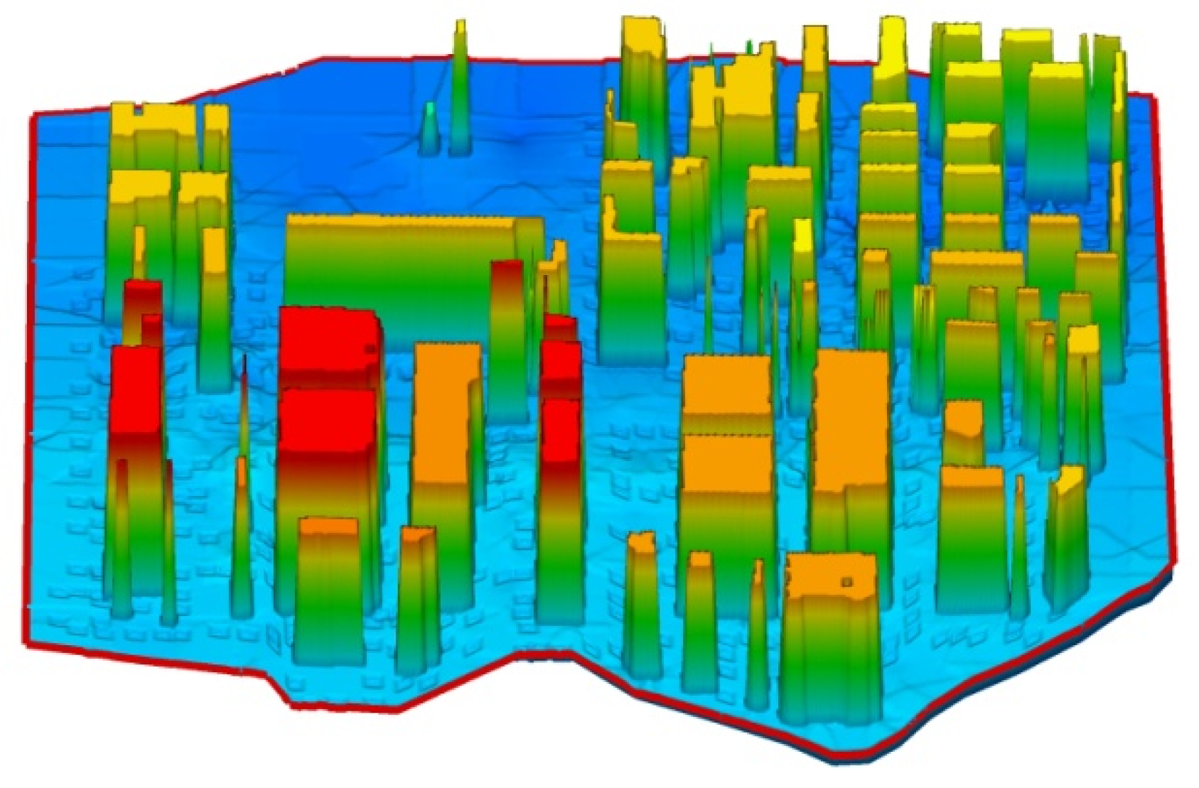
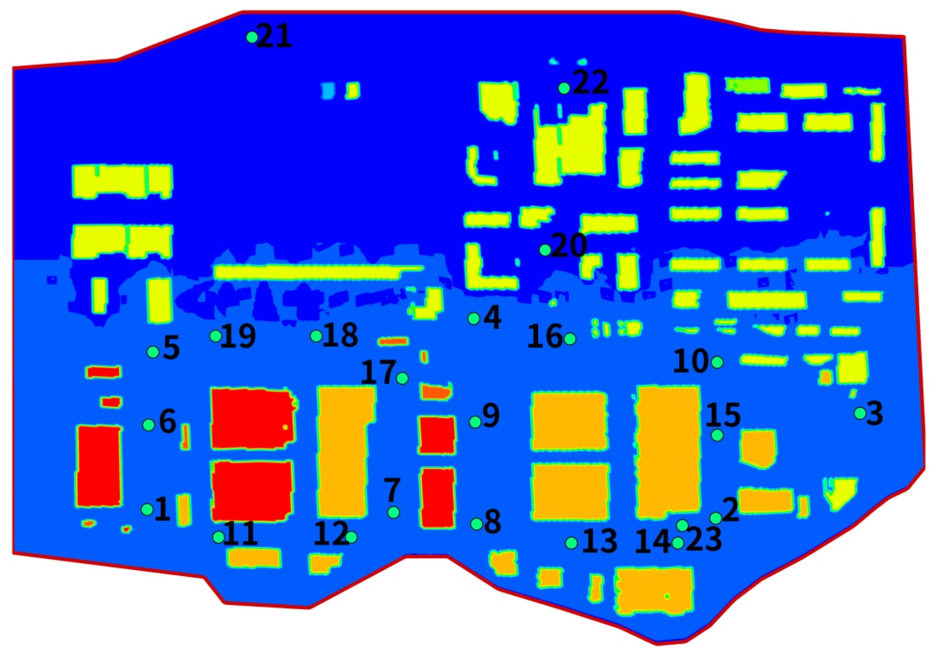
3.2.1. Generalized Building

The buildings were generalized according to the building layout of the nuclear power plant and its elevation, as shown in Figure 4.

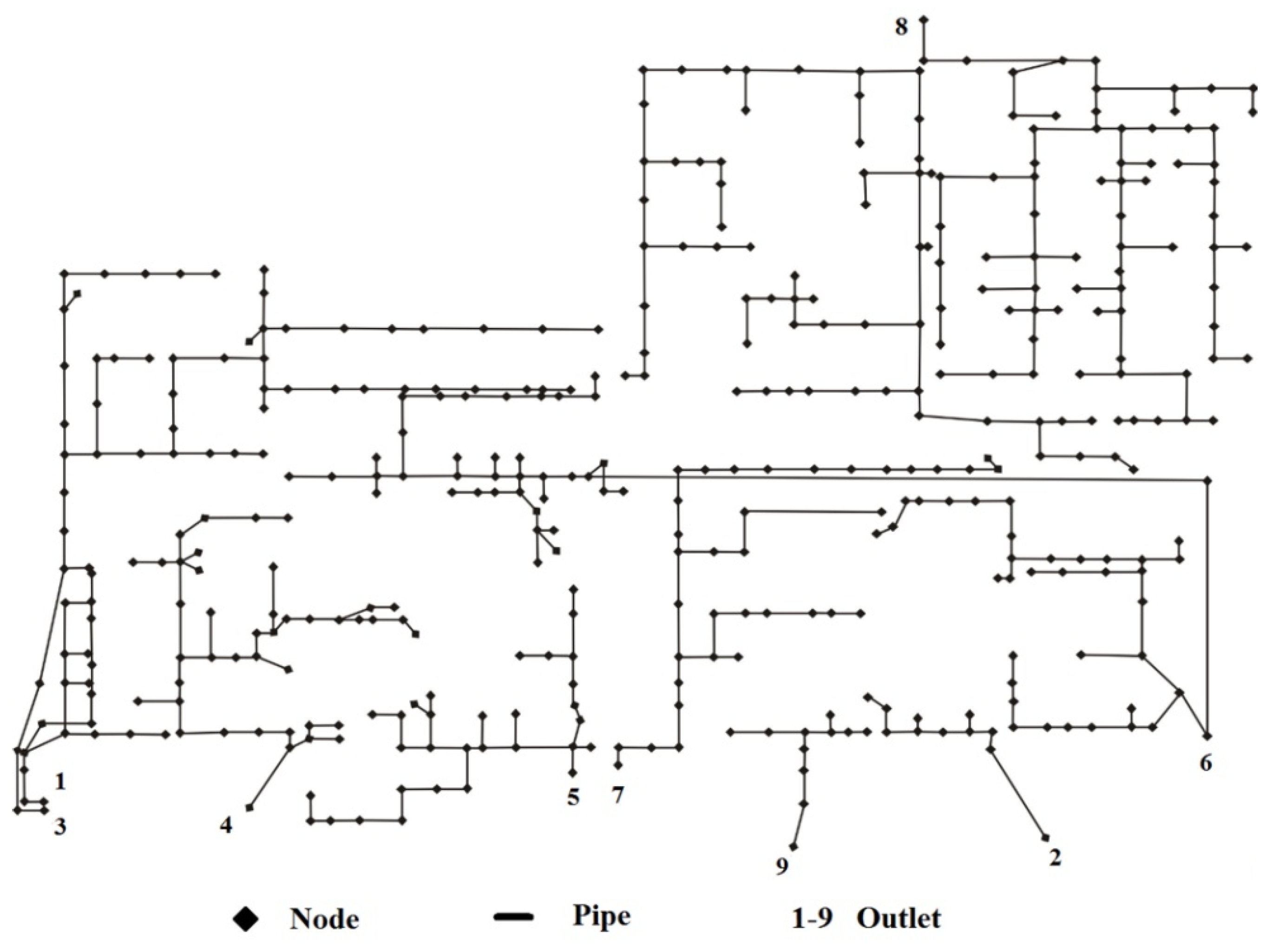
3.2.2. Generalized Drainage Pipe Network

The total area of the nuclear power plant is 652,000 m2. The vacant land area, which is the total area excluding the building area, is approximately 149,000 m2. The vacant land area was modeled as the flooded area in this study. The nuclear power plant has nine water outlets and one drainage ditch in the water pump room. The outline of the drainage pipe network was summarized according to the layout data of the nuclear power plant water wells and pipelines, as shown in Figure 5.

3.2.3. Grid Generation

The computational domain covers an area of 652,000 m2 and is divided into 173,641 rectangular grids (481 × 361), with the maximum grid measuring 6.5 m long and 6.00 m wide, and with the minimum grid measuring 2.17 m long and 2.00 m wide.

3.2.4. Wet and Dry Grid Treatment

For the dry-wet process in the computational domain, the grid freeze method was used. The dried, submersed, and wet water depth was set. When the depth of a certain grid unit was less than the dried water depth (0.005 m), these grids were frozen without participating in the calculation until they were submerged again. When the water depth was between, for example, more than 0.005 m and less than 0.05 m, for the dry water depth and wet water depth, respectively, the equations for these units were adjusted. Only the continuity equation was calculated, whereas the momentum equation was not calculated. When the water depth of the grid unit was greater than the wet water depth, the continuity and momentum equations were simultaneously calculated.

3.3. Model Input Parameters

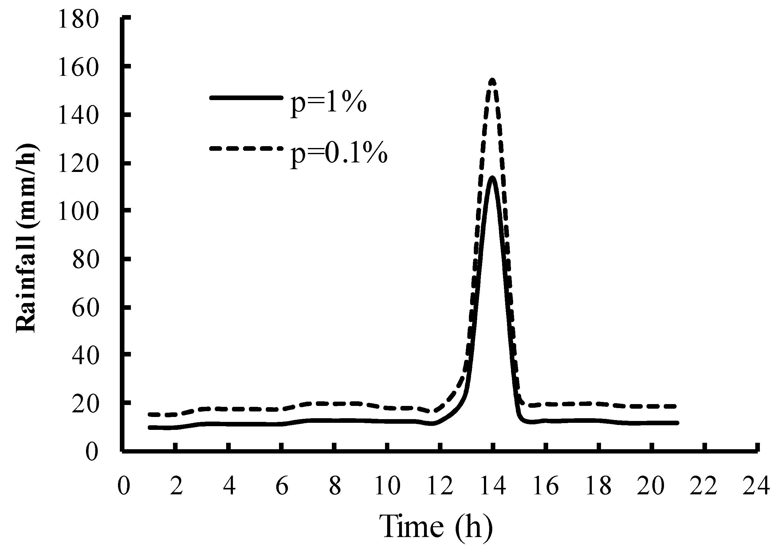
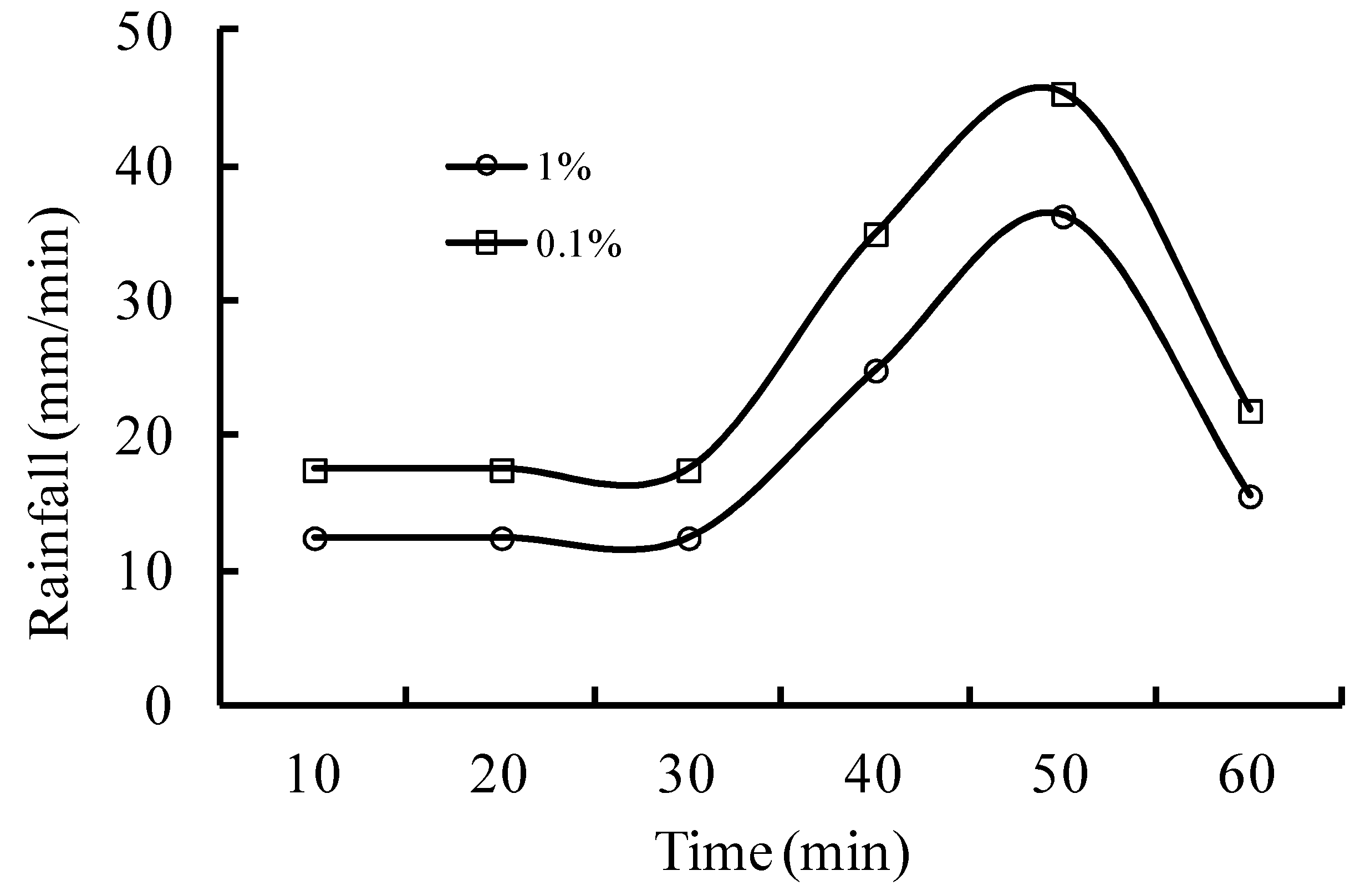
3.3.1. Rainfall and Wave Overtopping Data

The time distribution of the design storm was calculated based on the designed rainstorm data and the probable maximum precipitation (PMP) using the design storm distribution calculation method. This method considers the attenuation index and matches the index with calculation time. Based on the rainfall pattern distribution for three consecutive days (72 h), the third day, which was the day of maximum rainfall intensity (HIII = H24), was selected as the PMP of the nuclear power plant. The changing process of rainfall intensity over time was also expressed as the changing process of p over time t. The PMP of the plant at different rainfall durations is shown in Table 1, which reflects the corresponding relationship between accumulated rainfall (AR) and rainfall duration. The distribution of rainfall over 24 h and the distribution of rainfall within a maximum of 1 h in different rainfall conditions (p = 0.1 and 1%) are shown in Figure 6 and Figure 7, respectively.
The changing wave overtopping process in a typical seawall can be expressed as the changing process of the wave overtopping rate Qw over time t.
According to previous research results and engineering practice analyses [34,35], the overflow calculation should be set in the determination method, which, after considering embankment adjustment, ultimately establishes the high-water level of the site design as 10.01 m. To better assess and predict the safety of nuclear power plants, we assumed that heavy rainfall and overtopping flow occur simultaneously. The rainfall actually starts at the first hour and ends at 21 h (Figure 6). During the calculation, the design rainstorm distribution within 21 hours was included in the calculation, and the overtopping flow continued from 0 to 4 h (Table 2). Therefore, 1–4 hours is the time during which the heavy rainfall and the overtopping flow occur simultaneously. The wave overtopping rate of the three seawall sections at different times was simulated using the simulating waves nearshore model (SWAN), which can be used to calculate the generation, growth, and propagation of stormy waves in coastal waters. There are three typical seawall sections at the nuclear power plant, which are all located in the nuclear island area, that is Sections 1-1, 1-2, and 1-3 (Figure 8). Due to the protection of the reef, the wave overtopping rate of seawall Section 1-2 is relatively low. The total amount of wave overtopping for the three seawall sections is approximately 1.157 million m3, which combines the results of the largest typhoon wave calculation with the wave overtopping test results of typical seawall sections in the plant.

3.3.2. Initial and Boundary Conditions

The initial flow velocity and the water depth of surface runoff were zero. Thus, the initial flow velocity and the water depth of the pipe were zero [28].
Q t = 0 = 0 ,   u t = 0 = 0 ,   v t = 0 = 0 ,   h t = 0 = 0
where Q is the discharge in the pipe (m3/s), h is the water depth (m), and u and v are velocity components of velocity vector u in the x- and y-directions, respectively.
The boundary of the model includes the surface runoff as a moving boundary and the pipeline boundary.
(1)
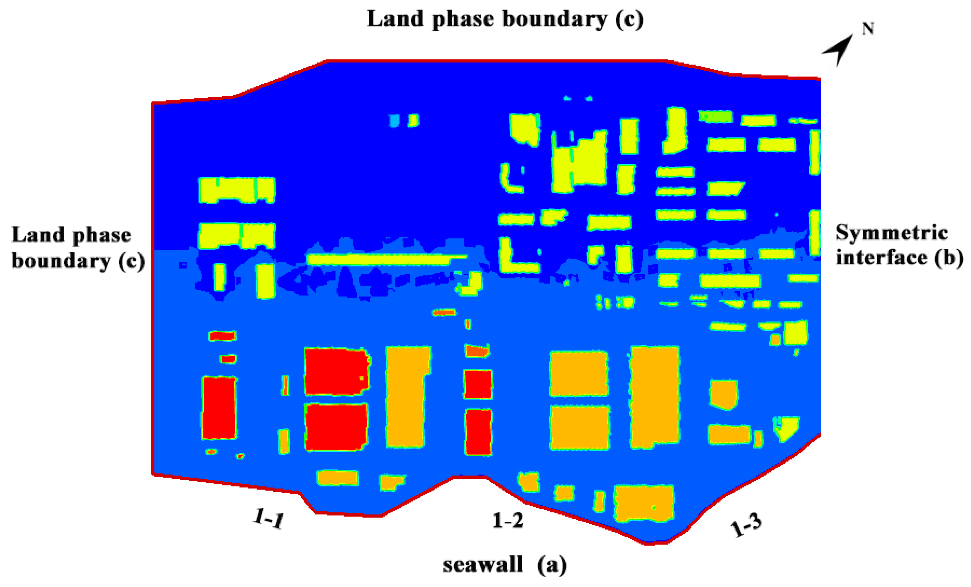
The surface boundary was divided into three parts: (a) the seawall boundary, (b) the symmetric interface of the plant, and (c) the land-phase boundary.
(a)
Seawall boundary: The seawall boundary refers to the inlet boundary given the wave overtopping rate.
(b)
Symmetric interface of the plant: The northeastern area of the nuclear power plant is relatively low, and the top of the breakwater embankment is higher than the elevation of the plant. Thus, the overtopping waves are large at this position, and the backwater affects the nuclear power plant. Another plant was constructed northeast of the nuclear power plant. Therefore, the northeastern boundary was considered the symmetric interface in the calculation. However, regardless of the backwater effect in the northeastern area, the normal velocity is zero for the nuclear power plant site at the interface.
(c)
Land-phase boundary: The land-phase boundary refers to the outlet border after considering the land elevation outside the boundary. This boundary is considerably lower than the elevation inside the plant. The water depth at point hi in the area, and the bottom level zi of the boundary, was calculated using the floodplain or weir flow formula [36]:
u n = { 0 h i z i 2 g ( h i z i ) h i > z i .
(2)
The pipeline boundary considers whether or not the pipe outlet is submerged. The flow or water level of the pipeline boundary is determined by the formulas for free and submerged discharge.

3.3.3. Pipeline Computational Conditions

The pipeline computational conditions were as follows: (1) the initial flow (Qin) and water depth (H) in the pipeline, (2) the inflow process of the catch-basin in the pipeline network (qb), and (3) the pipeline network outflow discharge process is the changing process of Qout over time t.

3.4. Numerical Discretization and Solution

The governing equations are discretized in the framework of the finite volume method (FVM). The convective flux on non-orthogonal, quadrilateral grids is evaluated using the second-order upwind scheme with a deferred correction [28]. The velocity–pressure coupling relationship is realized by using the SIMPLE algorithm based on the method described by Liu et al. [37].

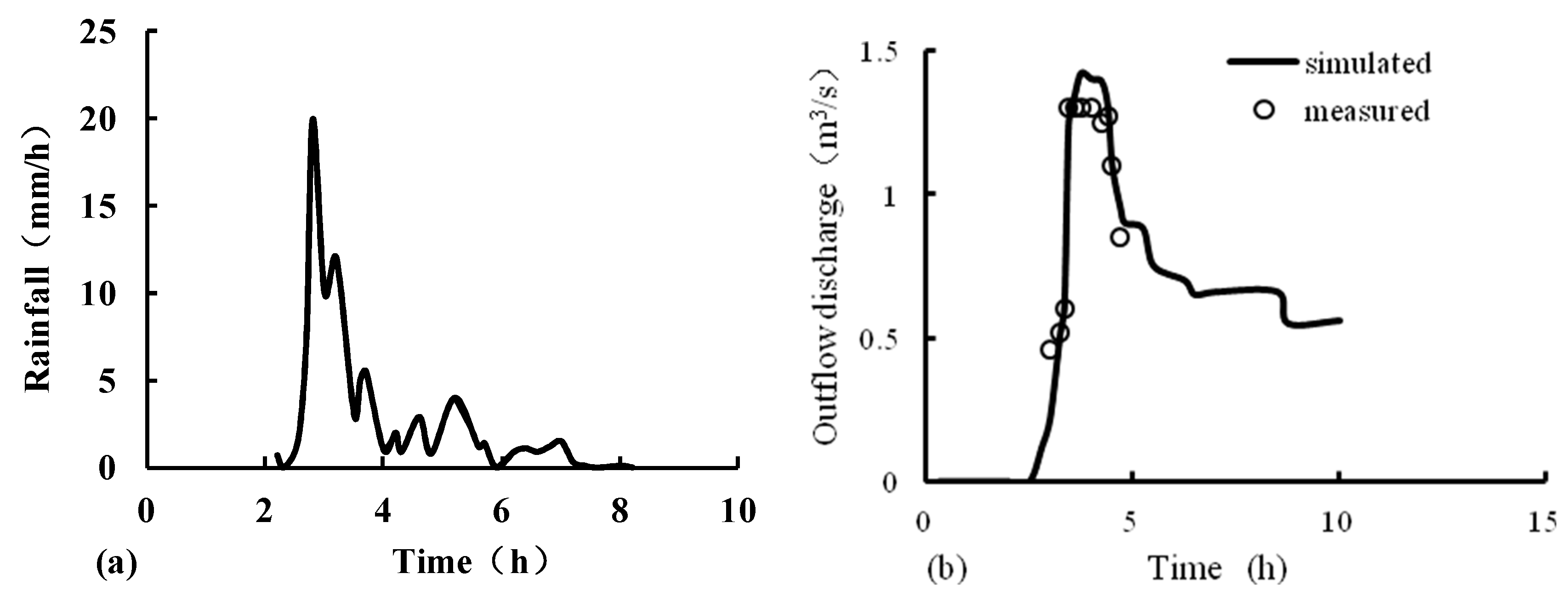
3.5. Model Validation and Calibration

The surface of the nuclear power plant uses different materials, so the roughness evidently varies along with the variation in the cross-section of the wetted perimeter. The roughness of different parts was calculated using a comprehensive roughness formula. The formula for calculating the comprehensive Manning roughness coefficient n is as follows:
When   n max n min > 1.5 2 , n = ( x 1 n 1 1.5 + x 2 n 2 1.5 + + x m n m 1.5 x 1 + x 2 + + x m )
When   n max n min < 1.5 2 , n = ( x 1 n + x 2 n 2 + + x m n m x 1 + x 2 + + x m )
where nmax and nmin are the maximum and minimum roughness for the same channel section, respectively, and x1, x2, …, xm are the wetted perimeters corresponding to each part of the roughness. The wetted perimeters are the boundary between the liquid and solid wall in the crossflow section.
The soil property and nuclear power plant surface protection material differ. Thus, according to the formula for calculating the comprehensive Manning roughness coefficient, the Manning coefficients of the pipe network and the land outside the pipe network are 0.02 and 0.035, respectively.
The model was validated using a heavy rainfall event that occurred on 23 June 2016. The rain lasted for six hours, and the total rainfall was approximately 96.7 mm. The outflow discharge and peak flow velocity of Water Outlet 1 were observed and simulated. The rainfall process is shown in Figure 9a. The outflow discharge of the pipeline validation results is shown in Figure 9b, and the peak flow velocity validation results are shown in Table 3.
The inundated water depth at the right of the plant was higher than the center and left of the plant, which is consistent with the actual measurements of the inundated water depth in each sub-area of the nuclear power plant during model validation (Figure 10). H is the inundated water depth (m) in Figure 10. Results showed that the rule for the outflow discharge of the pipeline and the peak flow velocity appropriately match the actual conditions and that the relative error of the peak flow velocity was within 20%. Thus, using the proposed model to study water depth in nuclear power plants is feasible.

4. Results and Discussion

To analyze the water depth in different locations of the nuclear power plant under different scenarios, 23 monitoring points in different locations of the plant were selected. The position of each monitoring point is shown in Figure 11.

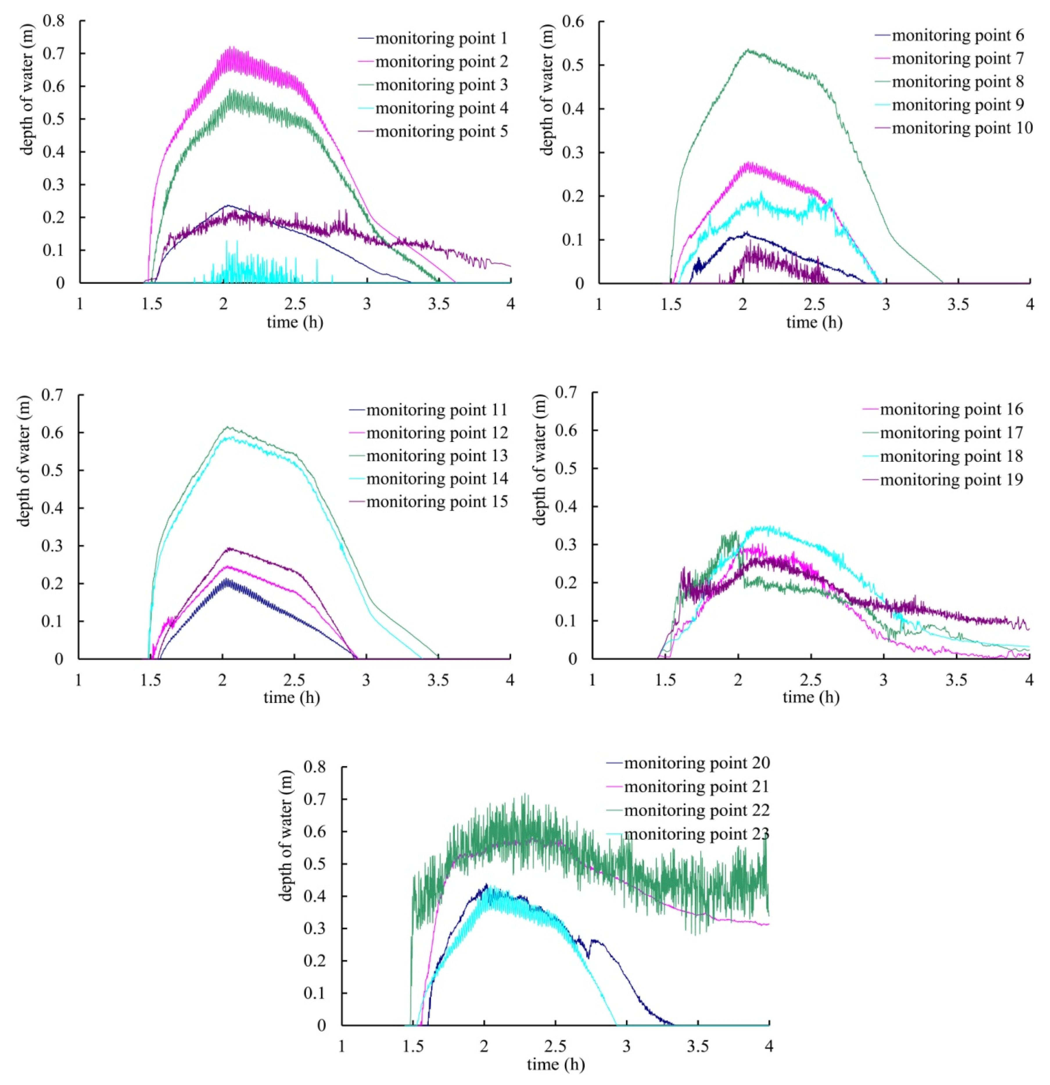
4.1. Temporal Distribution of Water Depth at the Nuclear Power Plant

In general, the inundated water depth right of the plant was higher than the center and left of the plant, reaching the maximum in approximately two hours. The water depth to the right of the plant was approximately 0.3–0.8 m, and the water depth to the left of the plant was approximately 0.2–0.4 m.
The south side of the nuclear plant is influenced directly by the wave overtopping rate. Thus, the inundated water depth in this area is higher than in other areas. The influences of the waves constrain rainwater drainage, resulting in deeper inundated water. The results also showed that the peak of the inundated water depth was high at all monitoring points, but the peak duration is short. From the point of the peak of inundated water depth, the water level was less than 11.63 m for the majority of the monitoring points. In our study, the peak of rainfall occurred at 14 h, and the results showed that stagnant water was present on the ground only in the first four hours (Figure 12). During the calculation, the design rainstorm distribution within 21 h was included in the calculation. The result indicated that the study area is more vulnerable to flooding due to wave overtopping than to flooding due to heavy rainfall. Corresponding to the tidal process, the wave overtopping rate of each seawall section in the wave process also increased first and then decreased, as shown by the wave overtopping rate for the three seawall sections at different times in Table 2. The peak of the wave overtopping rate and maximum inundated water depth of the nuclear power plant occurred at the same time (2 h). The water depth reached zero at about four hours (Figure 12).

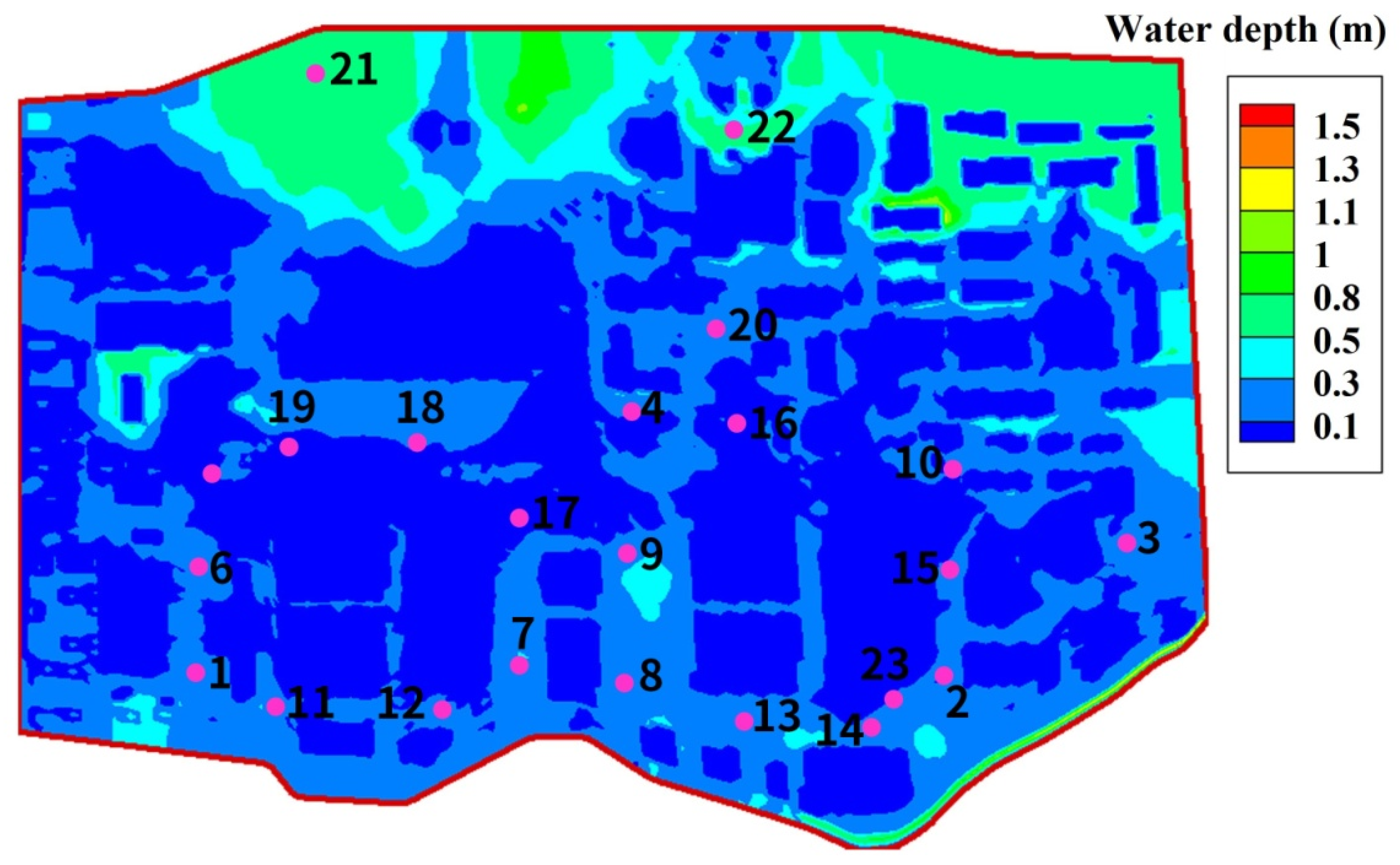
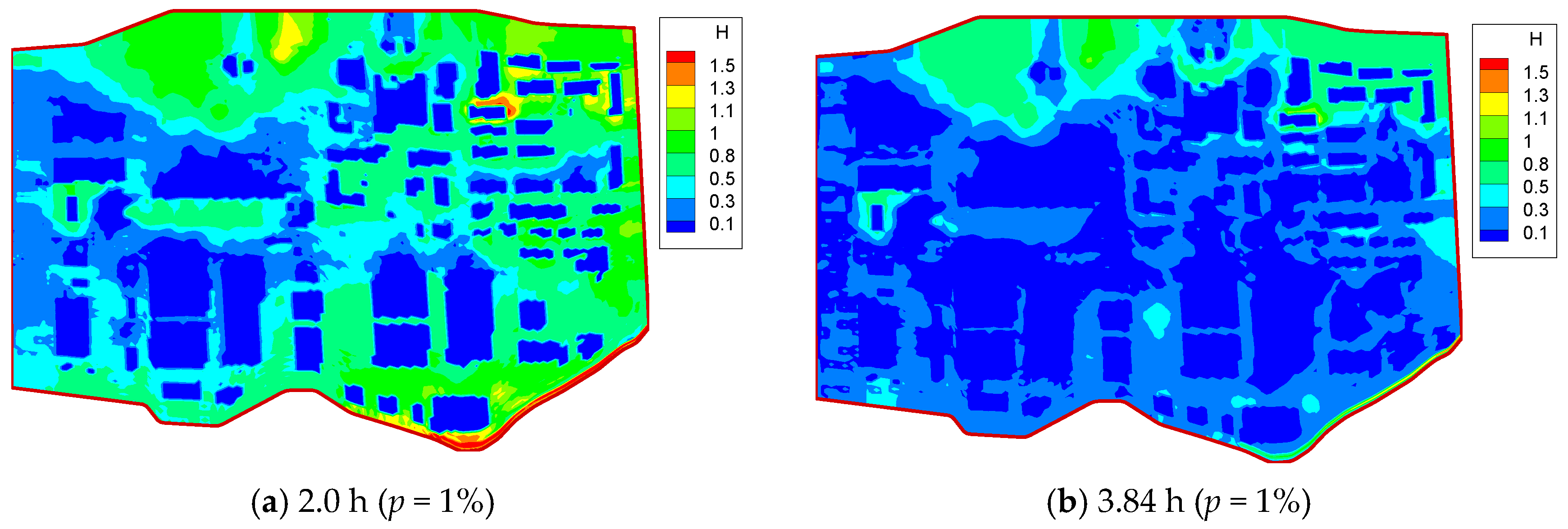
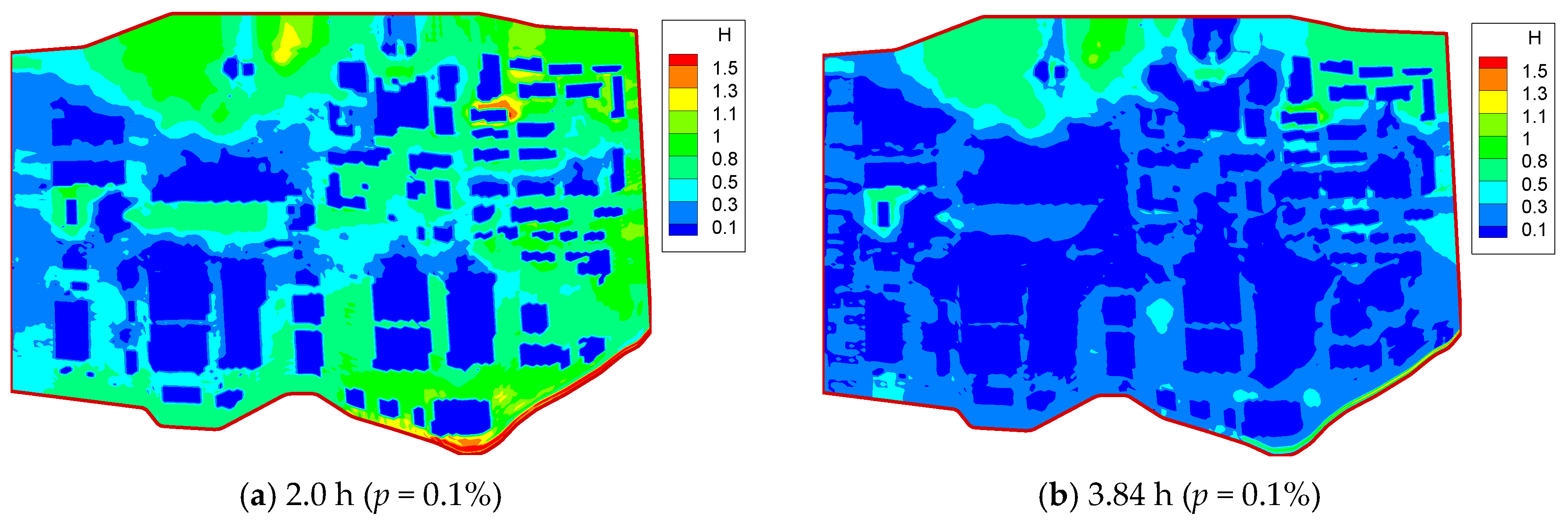
4.2. Spatial Distribution of Flooding Water at the Nuclear Power Plant

Under the combined effect of a designed once-in-a-century rainstorm (p = 1%) and the offshore design-based flood, the inundated water depth in the plant would be 0.12–0.72 m, and the maximum water depth of the 22 monitoring points would be 0.71 m (Figure 13). H is the inundated water depth (m). The inundated water depth would be 0.29–0.71 m at the nuclear island, and the inundated water depth of Monitoring Point 2 would be 0.71 m. The ground elevation of Monitoring Point 2 would be relatively high compared to the other points; thus, the deeper water at Monitoring Point 2 would not affect Monitoring Point 23. The inundated water depth for Monitoring Point 23 would be 0.42 m. The water depth curve of Monitoring Point 22 would vary due to the influence of the buildings.
Under the combined effect of a designed once-in-a-thousand years rainstorm (p = 0.1%) and the offshore design-based flood, the inundated water depth in the plant would be 0.13–0.75 m, and the maximum water depth of the 22 monitoring points would be 0.75 m. The water depth curve of Monitoring Points 19 and 22 would vary due to the influence of the buildings (Figure 14).
Monitoring Points 13, 14, 23, and 2 in the southeastern part of the nuclear power plant belong to the nuclear island area. The results show that the water depth of these monitoring points is relatively higher in different calculation schemes (Figure 12, Figure 13 and Figure 14). That is, the area near the nuclear island where the peak value of the water depth is higher, but the peak duration is short, so the temporary sealing and isolating method can be adopted in practical engineering to solve the problem of water accumulation in the nuclear island area. In addition, because of the low terrain in the right of the plant area, and the backwater may affect the nuclear island area. It is suggested that the way of sealing and isolating the area between the nuclear island area and the right side of the plant area should be used to solve the problem of back-flowing in the nuclear island area.
Based on the calculated spatial distribution of flood water at the nuclear power plant, different rainfall processes (p = 0.1, 1%) minimally influence the calculation results of the inundated water depth. The main factor influencing the flood water problem in a nuclear power plant is wave overtopping, which confirms the results of previous studies. Du et al. reported that wave overtopping is an important nearshore process that plays a vital role in nearshore morphological evolution and coastal flood disasters [38]. Lopes et al. observed that lagoon flood occurrences tend to be exacerbated under mean sea level rise scenarios, intensifying the landward intrusion [26].
In addition to taking some non-engineering measures (flood forecast etc.), some engineering measures should also be taken for the protection of extreme hydrological phenomena in this study area. Flood protection engineering measures usually include breakwaters, revetments, flood walls, and drainage facilities behind the breakwater around coastal nuclear power plants [21,22]. The design standards of flood control projects should be properly adjusted, appropriate structural designs should be adopted, various types of levees should be repaired and reinforced, drainage ditches should be provided inside the breakwaters, and seawater passing over the flood walls should be collected to the drain through the hardened drainage slopes. A drainage pipe from the ditch slope leading to the sea should be provided in the drainage ditch at an interval of 50 m, and the sea water over the embankment should be collected and discharged to the sea again. With the guarantee of engineering measures, the wave overtopping of the plant area should be reduced as much as possible to protect the critical infrastructure of nuclear power plants, so as to ensure the safety of nuclear power plant, reduce economic losses and casualties, and achieve the sustainable development of nuclear power plants.

5. Conclusions

The direct targets of flood disasters to human society include not only human beings but also the production and living facilities on which humans depend, which affects the sustainable development of the society, economy, and ecology. In this paper, a combined model was developed to simulate the flood process in a coastal nuclear power plant under the combined action of extreme rainfall and wave overtopping. We considered extreme rainfall and wave overtopping in the nuclear power plant as important input conditions for the model, including (1) the process of rainfall p with time t and (2) the progression of the wave overtopping rate QW with time t in typical seawall sections. Based on the above studies, the following conclusions can be drawn:
1. The peak wave overtopping rate and the maximum inundated water depth of the nuclear power plant occurred at the same time: two hours after the initiation of the heavy rainfall event. Therefore, the most important factor affecting the inundation in the plant area is wave overtopping.
2. The results showed that the water depth in the low-lying right area is deeper than that in other areas, which could cause backflow. This area was isolated for calculation, and the results indicated that back-flowing water can be prevented by sealing and isolating the middle portion of this area.
Given that the overtopping rate in our study is one of the boundary conditions for the surface 2D model, the descriptions for this part are relatively simple. On the basis of the results of this study, the inundated water depth of nuclear power plants should be studied in the future on the basis of the wave overtopping rate produced by different storm surges. The model of this study can simulate flooding inundation caused by wave overtopping and heavy rainfall at the nuclear power plant. Therefore, the numerical model can be employed as a tool for flood forecasting.

Author Contributions

S.W. acquired the data. S.W. and F.C. designed and wrote the paper. S.W. and W.Z. contributed to the conception of the paper and the interpretation of the data.

Funding

The authors are grateful for the financial support from the Guangdong Natural Science Foundation of China (2016A030312004), the International Science and Technology Cooperation Project (GASI-IPOVAI-04), the National Key Research and Development Plan (2016YFC1401403), and the Project of Enhancing School with Innovation of Guangdong Ocean University (GDOU2014050201, GDOU2013010203, GDOU2013050201, GDOU2013050215, GDOU2013050315).

Conflicts of Interest

The authors declare no conflict of interest.

References

  1. Tondel, M.; Granath, G.; Wålinder, R. 137 Cs activity in Sweden after the Chernobyl Nuclear Power Plant accident in relation to quaternary geology and land use. Appl. Geochem. 2017, 87, 38–43. [Google Scholar] [CrossRef]
  2. Fernández, D.S.; Lutz, M.A. Urban flood hazard zoning in Tucumán Province, Argentina, using GIS and multicriteria decision analysis. Eng. Geol. 2010, 111, 90–98. [Google Scholar] [CrossRef]
  3. Dewals, B.J.; Archambeau, P.; Duy, B.K.; Erpicum, S.; Pirotton, M. Semi-explicit modelling of watersheds with urban drainage systems. Eng. Appl. Comput. Fluid Mech. 2012, 6, 46–57. [Google Scholar] [CrossRef]
  4. Shibahara, S. The 2011 Tohoku Earthquake and Devastating Tsunami. Tohoku J. Exp. Med. 2011, 223, 305–307. [Google Scholar] [CrossRef] [PubMed] [Green Version]
  5. Hsu, M.H.; Chen, S.H.; Chang, T.J. Inundation simulation for urban drainage basin with storm sewer system. J. Hydrol. 2000, 234, 21–37. [Google Scholar] [CrossRef] [Green Version]
  6. Kopytko, N.; Perkins, J. Climate change, nuclear power, and the adaptation mitigation dilemma. Energy Policy 2011, 39, 318–333. [Google Scholar] [CrossRef]
  7. Dolif, G.; Engelbrecht, A.; Jatobá, A. Resilience and brittleness in the ALERTA RIO system: A field study about the decision-making of forecasters. Nat. Hazards 2013, 65, 1831–1847. [Google Scholar] [CrossRef]
  8. Rossman, L.A. Storm Water Management Model User’s Manual Version 5.0; National Management Research Laboratory Office of Research and Development U.S. Environmental Protection Agency Cincinnati: Cincinnati, OH, USA, 2004.
  9. Schmitt, T.G.; Thomas, M.; Ettrich, N. Analysis and modeling of flooding in urban drainage systems. J. Hydrol. 2004, 299, 300–311. [Google Scholar] [CrossRef]
  10. Fang, X.; Su, D.H. An integrated one-dimensional and two-dimensional urban stormwater flood simulation model. J. Am. Water Resour. Assoc. 2006, 42, 713–724. [Google Scholar] [CrossRef]
  11. Liu, X.Z.; Kang, S.Z.; Liu, D.L. A SCS model based on geography information and its application on rainfall runoff of typical small watershed on loess plateau. J. Hydrol. Eng. 2005, 24, 57–61. (In Chinese) [Google Scholar]
  12. Bruen, M.; Yang, J.Q. Combined hydraulic and black-box models for flood forecasting in urban drainage systems. J. Hydrol. Eng. 2006, 11, 589–596. [Google Scholar] [CrossRef]
  13. Tran, D.H.; Ng, A.W.M.; Perera, B.J.C. Neural networks deterioration models for serviceability condition of buried stormwater pipes. Eng. Appl. Artif. Intell. 2007, 20, 1144–1151. [Google Scholar] [CrossRef]
  14. Lin, B.L.; Wicks, J.M.; Falconer, R.A.; Adams, K. Integrating 1D and 2D hydrodynamic models for flood simulation. Water Manag. 2006, 159, 19–25. [Google Scholar] [CrossRef]
  15. Adeogun, A.G.; Pathirana, A.; Daramola, M.O. 1D-2D hydrodynamic model coupling for inundation analysis of sewer overflow. J. Eng. Appl. Sci. 2012, 7, 356–362. [Google Scholar] [CrossRef]
  16. Son, A.L.; Kim, B.; Han, K.Y. A simple and robust method for simultaneous consideration of overland and underground space in urban flood modeling. Water 2016, 8, 494. [Google Scholar] [CrossRef]
  17. Xie, J.; Wu, C.; Li, H.; Chen, G. Study on storm-water management of grassed swales and permeable pavement based on SWMM. Water 2017, 9, 840. [Google Scholar] [CrossRef]
  18. Yazdi, J. Water quality monitoring network design for urban drainage systems, an entropy method. Urban Water J. 2018, 15, 1–7. [Google Scholar] [CrossRef]
  19. Karim, M.F.; Tingsanchali, T. A coupled numerical model for simulation of wave breaking and hydraulic performances of a composite seawall. Ocean Eng. 2006, 33, 773–787. [Google Scholar] [CrossRef]
  20. Ebersole, B.A.; Westerink, J.J.; Bunya, S. Development of storm surge which led to flooding in St. Bernard Polder during Hurricane Katrina. Ocean Eng. 2010, 37, 91–103. [Google Scholar] [CrossRef]
  21. Hubbard, M.E.; Dodd, N. A 2D numerical model of wave run-up and overtopping. Coast. Eng. 2002, 47, 1–26. [Google Scholar] [CrossRef]
  22. Losada, I.J.; Lara, J.L.; Guanche, R. Numerical analysis of wave overtopping of rubble mound breakwaters. Coast. Eng. 2008, 55, 47–62. [Google Scholar] [CrossRef]
  23. Chen, X.; Ji, P.; Wu, Y.; Zhao, Y.; Zeng, L. Coupling simulation of overland flooding and underground network drainage in a coastal nuclear power plant. Nucl. Eng. Des. 2017, 325, 129–134. [Google Scholar] [CrossRef]
  24. Ren, X.; Yu, D.; Ruan, Y.; Yu, G. Modeling of municipal drainage and urban channel flooding in coastal city in the south of china. J. Risk Anal. Crisis Response 2015, 5, 74–86. [Google Scholar] [CrossRef]
  25. Hsu, T.W.; Shih, D.S.; Li, C.Y. A Study on Coastal Flooding and Risk Assessment under Climate Change in the Mid-Western Coast of Taiwan. Water 2017, 9, 390. [Google Scholar] [CrossRef]
  26. Lopes, C.L.; Dias, J.M. Assessment of flood hazard during extreme sea levels in a tidally dominated lagoon. Nat. Hazards 2015, 77, 1345–1364. [Google Scholar] [CrossRef]
  27. Karim, M.F.; Mimura, N. Impacts of climate change and sea-level rise on cyclonic storm surge floods in Bangladesh. Glob. Environ. Chang. 2008, 18, 490–500. [Google Scholar] [CrossRef]
  28. Zhang, W.S.; Zhao, Y.X.; Xu, Y.H. 2-D numerical simulation of radionuclide transport in the lower Yangtze River. J. Hydrodyn. 2012, 24, 702–710. [Google Scholar] [CrossRef]
  29. Ou, S.H.; Liau, J.M.; Hsu, T.W.; Tzang, S.Y. Simulating typhoon waves by swan wave model in coastal waters of Taiwan. Ocean Eng. 2002, 29, 947–971. [Google Scholar] [CrossRef]
  30. Akpınar, A.; Vledder, G.P.V.; Kömürcü, M.İ.; Özger, M. Evaluation of the numerical wave model (swan) for wave simulation in the black sea. Cont. Shelf Res. 2012, 50–51, 80–99. [Google Scholar] [CrossRef]
  31. Abott, M.B.; Madsen, P.A.; Sorensen, O.R. Scientific Documentation of Mike21 BW—Boussinesq Wave Module; MIKE by DHI: Hørsholm, Denmark, 2001. [Google Scholar]
  32. Panigrahi, J.K.; Padhy, C.P.; Murty, A.S.N. Inner harbour wave agitation using boussinesq wave model. Int. J. Nav. Archit. Ocean Eng. 2015, 7, 70–86. [Google Scholar] [CrossRef] [Green Version]
  33. Nasello, C.; Tucciarelli, T. Dual multilevel urban drainage model. J. Hydraul. Eng. 2005, 131, 748–754. [Google Scholar] [CrossRef]
  34. Reeve, D.E.; Soliman, A.; Lin, P.Z. Numerical study of combined overflow and wave overtopping over a smooth impermeable seawall. Coast. Eng. 2008, 55, 155–166. [Google Scholar] [CrossRef]
  35. Miao, Q.; Jiang, W.; Zhang, C.L. Common calculation methods of wave run-up and overtopping. Guangdong Water Resour. Hydropower 2008, 8, 11–13. (In Chinese) [Google Scholar]
  36. Vandenbroeck, J.M.; Keller, J.B. Weir flows. J. Fluid Mech. 1987, 176, 283–293. [Google Scholar] [CrossRef]
  37. Liu, S.H.; Luo, Q.S.; Mei, J.Y. Simulation of sediment-laden flow by depth-averaged model based on unstructured collocated grid. J. Hydrodyn. 2007, 19, 525–532. [Google Scholar] [CrossRef]
  38. Du, Y.; Pan, S.; Chen, Y. Modelling the effect of wave overtopping on nearshore hydrodynamics and morphodynamics around shore-parallel breakwaters. Coast. Eng. 2010, 57, 812–826. [Google Scholar] [CrossRef]
Figure 1. Sketch map of surface and underground coupling.
Sustainability 11 00642 g001
Figure 2. Flowchart for the numerical scheme.
Sustainability 11 00642 g002
Figure 3. Geographical position of the study area.
Sustainability 11 00642 g003
Figure 4. Three-dimensional (3D) stereogram of the buildings at the nuclear power plant.
Sustainability 11 00642 g004
Figure 5. Diagram of the generalized drainage pipe network at the nuclear power plant.
Sustainability 11 00642 g005
Figure 6. Designed 24-hour rainstorm distribution.
Sustainability 11 00642 g006
Figure 7. Distribution of rainfall within a maximum of 1 h.
Sustainability 11 00642 g007
Figure 8. Sketch map of the boundary conditions at the nuclear power plant.
Sustainability 11 00642 g008
Figure 9. (a) The rainfall process. (b) The outflow discharge of the pipeline validation results.
Sustainability 11 00642 g009
Figure 10. The flooded map of the nuclear power plant.
Sustainability 11 00642 g010
Figure 11. The position of each monitoring point in the nuclear power plant.
Sustainability 11 00642 g011
Figure 12. Temporal distribution of the water depth of the different monitoring points at the nuclear power plant.
Sustainability 11 00642 g012
Figure 13. Spatial distribution of flooding water at the nuclear power plant at different times (p = 1%).
Sustainability 11 00642 g013
Figure 14. Spatial distribution of flooding water at the nuclear power plant at different times (p = 0.1%).
Sustainability 11 00642 g014
Table 1. The probable maximum precipitation (PMP) of the nuclear power plant at different rainfall durations.
Rainfall Duration (h)0.5123456789101112
HPMP,AR (mm)185261364446514574628661691720746769790
Rainfall duration (h)131415161718192021222324
HPMP,AR (mm)8108308508708909089269439599749871000
Table 2. Wave overtopping rate of three seawall sections at different times.
Time (h)Tidal Level (m)Seawall Section 1-1Seawall Section 1-2Seawall Section 1-3
HS (m)Qw (m3/m/s)HS (m)Qw (m3/m/s)HS (m)Qw (m3/m/s)
0:006.041.4901.0302.120
1:008.992.750.0052.020.0013.450.05
1:309.763.600.102.790.064.210.23
2:0010.014.340.253.580.194.900.44
2:309.544.470.163.860.114.970.38
3:008.464.420.093.990.064.620.14
4:005.693.780.0013.560.0023.860.001
Note: HS is the incident wave height; Qw is the wave overtopping rate.
Table 3. The peak flow velocity validation results.
Time (h)Measured Value (m/s)Calculated Value (m/s)Relative Error
2:500.50.536%
3:451.251.19−4.80%
4:501.221.241.60%
5:100.80.9215%
7:201.241.413%

