Two-Stage Optimization Model for Two-Side Daily Reserve Capacity of a Power System Considering Demand Response and Wind Power Consumption

Abstract

Today, wind power is becoming an important energy source for the future development of electric energy due to its clean and environmentally friendly characteristics. However, due to the uncertainty of incoming wind, the utilization efficiency of wind energy is extremely low, which means the problem of wind curtailment becomes more and more serious. To solve the issue of wind power large-scale consumption, a two-stage stochastic optimization model is established in this paper. Different from other research frameworks, a novel two-side reserve capacity mechanism, which simultaneously takes into account supply side and demand side, is designed to ensure the stable consumption of wind power in the real-time market stage. Specifically, the reserve capacity of thermal power units is considered on the supply side, and the demand response is introduced as the reserve capacity on the demand side. At the same time, the compensation mechanism of reserve capacity is introduced to encourage generation companies (GENCOs) to actively participate in the power balance process of the real-time market. In terms of solution method, compared with the traditional k-means clustering method, this paper uses the K-means classification based on numerical weather prediction (K-means-NWP) scenario clustering method to better describe the fluctuation of wind power output. Finally, an example simulation is conducted to analyze the influence of reserve capacity compensation mechanism and system parameters on wind power consumption results. The results demonstrate that with the introduction of reserve capacity compensation mechanism, the wind curtailment quantity of the power system has a significant reduction. Besides, the income of GENCOs is gradually increasing, which motivates their enthusiasm to provide reserve capacity. Furthermore, the reserve capacity mechanism designed in this paper promotes the consumption of wind power and the sustainable development of renewable energy.

1. Introduction

1.1. Background and Motivation

With the excessive consumption of fossil energy, energy transformation has been paid attention by all countries worldwide. Renewable energy is favored because of its cleanness, environmental protection, and renewability [1]. Therefore, renewable energy generation will become the main method of electric energy production in the future. However, these clean energy sources also have some disadvantages. For instance, some kinds of renewable energy supply such as PV (photovoltaic) and wind power, due to the randomness and fluctuation during the generation process, will increase the volatility of system power generation output. What is more, with their large-scale penetration, the uncertainty of market balance will also increase, resulting in the power system operation facing serious challenges. For this reason, countries around the world have not been very effective in large-scale use of clean energy. In China, the utilization efficiency of wind energy is very low, and wind curtailment is a serious problem [2]. In 2017, the wind curtailment rate in Xinjiang and Gansu province reached 33% and 29% respectively [3]. Consequently, how to use renewable energy such as wind energy efficiently and reduce spillage of wind power is the main problem to be solved in this paper. Specifically, we further discuss the root cause of wind spillage, and we found that it is mainly the uncertainty of wind in nature that leads to the failure of accurate prediction of wind power output, which leads to the deviation of real-time wind power output, and finally affects the scheduling and production arrangement of the real-time spot market. In order to realize large-scale consumption of wind power, reserve capacity in the real-time stage is necessary, but a free reserve makes power generation companies gradually lose interest [4]. Therefore, the establishment of a compensation mechanism for reserve capacity will encourage more and more power generation manufacturers to provide more reserve capacity in the real-time stage, offer sufficient reserve space for wind power, and promote wind power consumption.

1.2. Literature Review

With large-scale wind power penetrating into the power system, the significant increase of the frequency modulation (FM) reserve unit is an inevitable trend [5]. However, considering the uncertainty of wind power, how to reasonably arrange the production of these reserve units is the main issue we need to focus on. In view of this problem, many studies have been done in previous research. The following is an overview of the methodology used by predecessors’ studies to solve this problem.

For the uncertainty processing of wind power, most of the processing methods adopted in the previous research can be divided into two categories, namely robust optimization and stochastic optimization. References [6,7,8,9,10] adopt the idea of robust optimization to cope with the volatility of wind power. Reference [6] studies the wind power uncertainty of gas-electric integrated system coordination optimization and puts forward a two-stage distributionally robust optimization (DRO) model with the goal of minimum system total operating cost to analyze the impact of residents of gas load, abandon the wind punishment cost coefficient, and climb rate parameters on the final optimization results. Based on robust optimization, the literature [7] establishes an optimization model for joint scheduling of energy and auxiliary services markets that considered wind power uncertainty in the real-time power market and proposes redundant constraint reduction strategy to improve the computational efficiency of robust joint scheduling. Reference [8] utilizes distributionally robust chance constrained and interval optimization to handle the impact of wind power fluctuation. In reference [9], a robust unit commitment model with multi objectives (minimizing the operating cost and maximizing the peak shaving capacity of the power system) is proposed to resist the disturbance of wind power stochastic fluctuation. In addition, reference [10] utilizes robust optimization to deal with the uncertainty of wind power and photovoltaic power output, and the Gaussian process method is used to predict the confidence interval of uncertain parameters, which support a day-ahead market scheduling strategy formulation. However, both robust optimization and distributionally robust optimization have drawbacks, which are that scheduling decisions are too conservative and at the expense of economic interests.

Therefore, stochastic optimization, another method to solve uncertain problems, is favored by researchers. Reference [11] formulates a stochastic optimization model to accomplish the day-ahead economic dispatch fully considered wind power volatility. In reference [12], a scheduling model for the coordinated operation of hydro and wind power is established by utilizing the complementary characteristics of hydro and wind energy, and a stochastic programming model is adopted to cope with the uncertainty of wind power output. In addition, reference [13], in considering the influence of solar radiation intensity and wind power uncertainty on the whole scheduling process, establishes a stochastic optimal scheduling model for centralized wind-solar power stations. Moreover, a day-ahead stochastic scheduling model of thermal-hydro-wind-photovoltaic power system is presented in reference [14], which adopts Monte Carlo simulation to generate the output scenarios of wind power and photovoltaic power to describe their uncertainty. Yet all of the above studies did not consider the impact of wind power uncertainty on the power system concretely. Specifically, wind power in the electricity spot market is divided into two stages, i.e., the first stage is day-ahead market dispatch phase, and the second stage is a real-time market, whereas the actual deviation of the wind power output often occurs in the second stage. Therefore, the established stochastic programming model divided into two stages should be taken into account, which can restore the real-time situation of actual scheduling.

Generally, the consumption of wind power not only considers the reserve capacity market but also other methods to realize the safe and reliable connection of wind power to the grid. For example, demand response management (DRM) [15], joint operation of energy storage units, and other cooperative operation mechanism can balance the deviation of wind power real-time output. However, many researchers tend to consider these in terms of reserve capacity and ignore other approaches that can also promote wind power consumption. In reference [16], a dynamic economic scheduling model of integrated power system contained wind power is proposed to optimize the generation and reserve capacity of all units, and the capacity and ramp rate of the generator have an important impact on the optimal scheduling of reserve capacity, but the demand response of the user side is not mentioned. What is more, reference [17] introduces the concept of interruptible load and presents a cost-benefit tradeoff-based algorithm for optimal reserve capacity in the power market, which emphasized that both generator sets and interruptible load could participate in the reserve market. In addition, some of the literature also adopts the joint operation of energy storage device and wind turbine to reduce the interference of wind power instability on the system [18,19,20]. For instance, reference [18] proposes a wind power, pumped storage, and thermal plant joint operation mechanism with the objective of maximizing the operator’s profit gained from the day-ahead market and reserve market, and a heuristic optimization algorithm has been used to solve this problem. In reference [19], a combination of wind turbines and air compression energy storage devices is introduced. Similar to reference [18], reference [20] also presents a decision-making mechanism for wind-energy storage joint system to participate in day-ahead market and reserve market. In summary, it can be found that the research on the scheduling mechanism of DRM as a flexible resource to balance wind power is relatively weak. Consequently, it is necessary to fill the research gap in this field.

According to the summary of the above literature review, it can be obviously concluded that previous research still has three insufficiencies. First of all, in terms of research methods, most of them adopt the idea of robust optimization, which leads to the over-conservative results. Second, the traditional stochastic optimization process cannot fully reflect the actual scheduling process when dealing with the uncertainty of wind power. Finally, on the demand side, the utilization of flexible demand response resources is insufficient.

1.3. Contributions and Organization

To fill the research gap, this paper proposes a novel two-stage stochastic optimization model for a wind power system with the participation of spot market, which considers both the flexibility of supply side and demand side, that is, the flexibility capacity includes interruptible load of demand response and reserve capacity of thermal power unit. The promotion effect of adding flexible capacity market in the real-time stage on the consumption of clean energy is fully studied, and the consumption situation of wind power is further analyzed. Additionally, the main contributions of this paper can be divided into three aspects. First, the model is constructed to establish a compensation mechanism when standby power is invoked in the real-time stage. Second, a two-stage stochastic optimization method is used to set up the scheduling optimization model, and the clustering method K-means-NWP is adopted to describe the uncertainty of wind power output. Finally, the flexibility of adjusting resources based on demand response is considered, which can increase the reserve power of the system and improve the consumption capacity of wind power.

Besides, the organization of the remaining sections are as follows: Section 2 elaborates the main problems studied in this paper; in the Section 3, the mathematical model is built and the solution method is given; Section 4 uses a numerical example to verify the rationality of the established model; and the final conclusions are given in Section 5.

2. Problem Description

In this section, the main problem that needs to be addressed in this paper is described in detail, which contains the main problem introduction and the proposed optimization method process.

2.1. Wind Power Consumption

With the rapid development of renewable energy sources (wind power, photovoltaic, etc.) in China, wind power installed capacity increases year by year. In order to implement the large-scale consumption of wind power and ensure the safe and stable operation of the power system, the power system needs to arrange a certain rotation reserve based on the original operation mode to cope with the uncertainty of wind power output [21]. The influence of wind power on system dispatch and operation is mainly caused by the uncertainty of wind power output, which changes rapidly and violently and is unpredictable. The previous method of reserve configuration cannot meet the new requirements brought by large-scale wind power grid connection [22]. With the increasing proportion of wind power being grid-connected, the demand for a spinning reserve is increasing. It is not enough to rely on conventional power supply to adjust and provide a spinning reserve. Therefore, how to fully exploit the other regulatory resources in the system and rationally optimize the rotating standby according to the characteristics of the spinning reserve requirements of a wind power grid-connected system is an urgent problem that needs to be solved [23]. At present, flexible capacity resources (like the reserve capacity of thermal power units, demand response, energy storage, etc.) are the key to solving the problem of wind power consumption. This paper mainly considers the impact of thermal power unit flexibility, demand response, and wind penalties on wind power consumption.

In order to ensure the safety and stability of the system, accept more clean energy, and maintain a good system operation economy, it is urgent to make a reasonable and effective decision on the optimization of spinning reserve capacity of the system after large-scale wind power integration.

2.2. Proposed Capacity Optimization Configuration Process

In this paper, a two-stage stochastic optimization model for dual-side reserve capacity of power system considering wind power consumption is proposed. The overall goal of two-side reserve capacity focuses on minimizing the total cost of system operation and improving wind power consumption. Specifically, the stochastic optimization model can be divided into two stages. In the first stage, in the day-ahead market, the dispatching operator sorts the operating costs and spare capacity costs reported by each generator unit and determines the spare capacity that can be provided in the market on the next day. Then, according to the forecast value of wind power output, the dispatching operator calculates the reserve capacity that needs to be reserved for each generator unit in the second stage. In the second stage, the method of randomly generating the scene is used to simulate the operation of the market on the next day. When the wind power has error fluctuation, each generator unit provides backup power for its system and at the same time considers the interruptible load on the demand side to provide the unit with backup power. Finally, the impact on wind power consumption is analyzed by introducing abandonment penalty cost, demand response, and thermal power unit flexibility (climbing rate, minimum technical output) in the objective function.

3. Mathematical Modeling and Solution

In this section, we present a two-stage stochastic optimization model that mainly focuses on optimizing the dual-side reserve capacity of the power system to improve wind power consumption. In the first stage, the wind power output is predicted to determine the system backup capacity that needs to be generated in the second stage. In the second stage, the wind power output is clustered according to historical meteorological data by the K-means-NWP method in order to simulate the wind power output on the next day, then according to the error between the wind power output simulation value and the actual value. The remaining reserve capacity in the day-ahead phase can be utilized to balance the error.

3.1. Mathematical Modeling

This paper presents a two-stage stochastic optimization model. In the first stage, the independent system operator (ISO) ranks the operation cost and reserve capacity cost reported by each unit in the day-ahead market. With the aim of minimizing the total operating cost of the system, the reserve capacity available on the intra-day market the next day can be determined by optimization [24]. Then according to the typical output scenario of wind power output, the reserve capacity provided by other units is calculated. In the second stage, the K-means method based on meteorological data is used to simulate the operation of the intra-day-market in the second day. In case of fluctuations in wind power, thermal units provide reserve capacity for the system, and meanwhile, interruptible load on the demand side is considered to provide reserve electricity (interruptible load refers to the load that can be interrupted by the user side when the power grid needs it, which is usually realized by signing a contract with the user). Considering the compensation price of reserve electricity supply from thermal unit and interruptible load in real-time market, the scheduling and production arrangement in the second stage is completed with the objective function of minimum system equilibrium in the real-time stage [25]. Finally, the effect on wind power consumption is analyzed by introducing penalty coefficient of wind curtailment, demand response, and flexibility of thermal units (ramp rate and minimum technical output) into the objective function.

$$\begin{array}{l}f=min{\displaystyle \sum _{t=1}^T{\displaystyle \sum _{g=1}^{N_G}[a_i}}{(P_{g,t}^{Da})}^2+b_i{P}_{g,t}^{Da}+c_i+{\mu }_{g,t}^{on}{C}_g^{start}+{\mu }_{g,t}^{off}{C}_g^{down}+{\rho }_{g,r}^u{R}_{g,t}^{up,max}+{\rho }_{g,r}^d{R}_{g,t}^{down,max})]+\\ {\displaystyle \sum _{\omega =1}^{\Omega }{\rho }_{\omega }{\displaystyle \sum _{t=1}^T{\displaystyle \sum _{g=1}^{N_G}\{}}(1-\omega ){\lambda }_t{R}_{\omega ,t}^{IL}+{\rho }_c^u{R}_{g,t}^{\omega ,up}+{\rho }_c^d{R}_{g,t}^{\omega ,down}+c^s{W}_{\omega }^{spill}\}}\end{array}$$

(1)

where a_i, b_i, c_i respectively represent the coefficients of the generating cost function of thermal units; ${\mu }_{g,t}^{on}$, ${\mu }_{g,t}^{off}$ denote the start and stop status of thermal units; ${\rho }_{g,r}^u$, ${\rho }_{g,r}^d$ refer to the compensation price of reserve capacity of thermal units; ${\rho }_{\omega }$ is the probability of wind power combination scenario $\omega$; $\Omega$ represents the total number of wind power combination scenarios, which equals to the product of the number of output scenes of all wind turbines; ${\lambda }_t$ is the user electricity price; ${\rho }_c^u$, ${\rho }_c^d$ represent the compensation price of standby power provided by thermal units in the real-time stage; $c^s$ denotes the penalty coefficient of wind curtailment; $W_{\omega }^{spill}$ represents the wind abandon quantity of wind power combination scenario $\omega$.

3.1.1. The Constraints of the Day-ahead Stage

(1)

Day-ahead system power balance

$${\displaystyle \sum _{g=1}^{N_G}{\displaystyle \sum _{w=1}^{N_w}(P_{g,t}^{Da}+P_{w,t}^{Da})=}}{L}_t,$$

(2)

where $N_G,N_W$ respectively represent the number of thermal power and wind power units. $P_{g,t}^{Da}$ is the power of thermal power unit g at time t in the day-ahead stage. $P_{w,t}^{Da}$ denotes the power of the wind turbine g at time stage t in the day-ahead stage. $L_t$ refers to the total load of the system at time t.

(2)

Day-ahead unit output constraint

$${\mu }_{g,t}{P}_g^{\mathit{min}}\le P_{g,t}^{Da}\le {\mu }_{g,t}{P}_g^{\mathit{max}},$$

(3)

where ${\mu }_{g,t}$ is the start and stop state of thermal unit g at time stage t. $P_g^{max}$, $P_g^{min}$ separately denote the maximum and minimum power of thermal unit g.

(3)

Day-ahead wind power output constraints

$$0\le P_{w,t}^{Da}\le {\stackrel{⌢}{P}}_{w,t},$$

(4)

where ${\stackrel{⌢}{P}}_{w,t}$ is the predictive power of wind turbine w at time stage t.

(4)

Day-ahead wind power ramping constraints

$$-r_w^d\le P_{w,t}^{Da}-P_{w,t-1}^{Da}\le r_w^u,$$

(5)

where $r_w^u$, $r_w^d$ refer to the ramp rate of wind turbine w.

(5)

Day-ahead thermal units startup and shut off constraints [26]

$${\mu }_{g,t}^{off}={\mu }_{g,t-1}-{\mu }_{g,t}+{\mu }_{g,t}^{on}$$

(6)

$${\mu }_{g,t}^{on}+{\mu }_{g,t}^{off}\le 1$$

(7)

(6)

Day-ahead thermal units ramping constraints

$$P_{g,t}^{Da}-P_{g,t-1}^{Da}\le r_g^u,$$

(8)

$$-r_g^d\le P_{g,t}^{Da}-P_{g,t-1}^{Da},$$

(9)

where $r_g^u$, $r_g^d$ refer to the ramp rate of thermal unit w.

(7)

Day-ahead spinning reserve capacity constraints

Upper reserve capacity provided by thermal units at time stage t:

$$R_{g,t}^{up,max}=min\{P_g^{max}-P_{g,t}^{Da},r_g^u\}.$$

(10)

Lower reserve capacity provided by thermal units at time stage t:

$$R_{g,t}^{down,max}=min\{P_{g,t}^{Da}-P_g^{min},r_g^d\}.$$

(11)

Lower reserve capacity required by wind turbine:

$$R_{w,t}^{down}=max\{{\displaystyle \sum _{k=1}^{K}P\{\delta (k)\}}{\stackrel{⌢}{P}}_{w,t},0\}.$$

(12)

Upper reserve capacity needed by wind turbine:

$$R_{w,t}^{up}=min\{{\displaystyle \sum _{k=1}^{K}P\{\delta (k)\}}{\stackrel{⌢}{P}}_{w,t},0\},$$

(13)

$${\displaystyle \sum _{g=1}^{N_G}{R}_{g,t}^{up,max}\ge {\displaystyle \sum _{w=1}^{N_W}{R}_{w,t}^{up}}},$$

(14)

$${\displaystyle \sum _{g=1}^{N_G}{R}_{g,t}^{down,max}\ge -{\displaystyle \sum _{w=1}^{N_W}{R}_{w,t}^{down}}},$$

(15)

where $R_{g,t}^{up,max}$ and $R_{g,t}^{down,max}$ respectively refer to the maximum of the upper reserve capacity and lower reserve capacity provided by thermal unit g at time stage t. $R_{w,t}^{up}$, $R_{w,t}^{down}$ separately refer to the maximum of the upper reserve capacity and lower reserve capacity required by wind turbine w at time stage t.

3.1.2. Real-time stage

(8)

Wind power abandon quantity constraint

$$0\le W_w^{spill}\le P_{w,t}^{Rt},$$

(16)

$$W_{\omega }^{spill}={\displaystyle \sum _{w=1}^{N_W}{W}_w^{spill}},$$

(17)

where $P_{w,t}^{Rt}$ is the power of wind turbine w at time stage t in the real-time stage; $W_w^{spill}$ refers to the wind abandon quantity of wind turbine w.

(9)

Real-time units output constraints

$$P_{g,\omega ,t}^{Rt}=P_{g,t}^{Da}+R_{g,\omega ,t}^{up}-R_{g,\omega ,t}^{down},$$

(18)

$${\mu }_{g,t}{P}_g^{max}\le P_{g,\omega ,t}^{Rt}\le {\mu }_{g,t}{P}_g^{min},$$

(19)

where $P_{g,\omega ,t}^{Rt}$ denotes the power of thermal unit g at time stage t in the wind power combination scene w at the real-time stage. $R_{g,\omega ,t}^{up}$ and $R_{g,\omega ,t}^{down}$ separately denote the upper reserve capacity and lower reserve capacity provided by thermal unit g at time stage t in the wind power combination scene w at the real-time stage.

(10)

Real-time reserve capacity constraints

$$R_{w,\omega ,t}^{up}\le R_{g,\omega ,t}^{up}\le u_{g,t}^{up}{R}_{g,t}^{up,max},$$

(20)

$$R_{w,\omega ,t}^{down}\le R_{g,\omega ,t}^{down}\le u_{g,t}^{down}{R}_{g,t}^{down,max},$$

(21)

where $u_{g,t}^{up}$ and $u_{g,t}^{down}$ respectively refer to the state provided by thermal unit g at time stage t in the real-time stage.

$$0\le R_{\omega ,t}^{IL}\le \theta L_t,$$

(22)

where $R_{\omega ,t}^{IL}$ denotes the interruptible load provided by users at time stage t in the wind power combination scenario $\omega$ in the real-time stage. $\theta$ represents the proportion of the maximum of interruptible load that can be provided by the power side to the total load [27].

(11)

Real-time reserve service (only one in use at any given time)

$$0\le u_{g,t}^{up}+u_{g,t}^{down}\le 1$$

(23)

(12)

Real-time wind power output constraints

$$\begin{array}{l}0\le P_{w,t}^{Rt}\le P_{w,t}^{Rt}\\ 0\le P_{w_2,t}^{Rt}\le P_{w_2,l,t}^{Rt}\end{array}$$

(24)

(13)

Real-time wind power ramping constraints

$$-r_w^d\le P_{w,t}^{Rt}-P_{w,t-1}^{Rt}\le r_w^u$$

(25)

(14)

Real-time power balance constraints

$${\displaystyle \sum _{g=1}^{N_G}(R_{g,\omega ,t}^{up}-R_{g,\omega ,t}^{down})}+R_{g,\omega ,t}^{IL}+{\displaystyle \sum _{w=1}^{N_W}(P_{w_1,s,t}^{Rt}+P_{w_2,l,t}^{Rt}-P_{w_1,t}^{Da}-P_{w_2,t}^{Da})}-W_{\omega }^{spill}=0$$

(26)

3.2. K-Means Classification Based on Numerical Weather Prediction (K-Means-NWP)

The K-means clustering method is the most classic one in the dynamic clustering algorithm. Its basic idea is to divide each sample into the category closest to the mean, which is clustered by the distance and near distance.

The K-means clustering algorithm generally includes the following processing steps:

(a)

Dividing all data into K initial classes, selecting K sample points as the initial cluster center, and record as $z_1(l),z_2(l)\dots \dots z_k(l)$; Where, the initial value $l$ = 1;

(b)

All samples are assigned to the K ${\omega }_j(K)$ class represented by each cluster center according to the nearest neighbor rule, The number of samples included in each category is $N_j(l)$;

(c)

Calculating the mean vector of each type and use the vector as the new cluster center:

$$z_j(l+1)=\frac{1}{N_j(l)}{\displaystyle \sum _{x(i)\in {\omega }_j(l)}x(i)},$$

(27)

where $j=1,2\dots \dots k,i=1,2\dots \dots N_j(l)$;

(d)

When $z_j(l+1)\ne z_j(l)$, it means the clustering result is not optimal, then returns to step (b) and continues the iterative calculation;

(e)

When $z_j(l+1)=z_j(l)$, it means that the clustering result is optimal at this time and the iteration process is over.

According to the literature [28], there is a close relationship between wind power generation and meteorological data, especially with wind speed. However, the existing statistical forecasting methods based on numerical weather forecast do not classify meteorological information according to different characteristics; that is, they do not consider the different characteristics of wind power output corresponding to different meteorological data. Therefore, it is necessary to solve the following problems: 1) different characteristics of meteorological information correspond to large differences in wind power output, and 2) various factors in meteorological data are related to wind power output; that is, the factors that play a leading role in wind power output. Based on this, this paper comprehensively considers various meteorological factors and proposes a method of wind power output prediction based on fuzzy k-means of numerical weather forecast (K-means-NWP). The specific steps are as follows:

Step 1

The meteorological factors affecting wind power output are analyzed, including daily atmospheric pressure average (Pav), daily wind speed minimum (Vim), daily wind speed maximum (Vmax), daily temperature minimum (Tmin), daily temperature maximum (Tmax), and daily wind direction, the sinusoidal mean (Dsin), and the daily wind cosine mean (Dcos).

Step 2

Select the historical meteorological data of the previous month, $x_i=[Pav\mathrm{Vmin}\mathrm{Vmax}\mathrm{Tmin}\mathrm{Tmax}\mathrm{Dsin}\mathrm{Dcos}]$, then $X=[x_1;x_2\dots \dots ;x_n];n=30$. Since the dimensions of the components in the NWP vector are different, normalization is required. The air pressure, wind speed, and temperature are divided by their respective historical maximum values. The wind direction sine and cosine values are normalized values and need no further processing.

Step 3

Set the initial value k of clustering number according to the number of target clusters.

Step 4

According to Equation (27), calculate the mean vector of each type and use the vector as the new cluster center.

Step 5

According to the fuzzy k-means criterion, judge the final result. If it is not the optimal result, return to step 4 to continue the iteration. Otherwise, the iteration ends, and the clustering result is output.

Step 6

Observe the meteorological data of the target day, calculate the distance between them and the clustering results and normalize them as the membership degree of the corresponding clustering results.

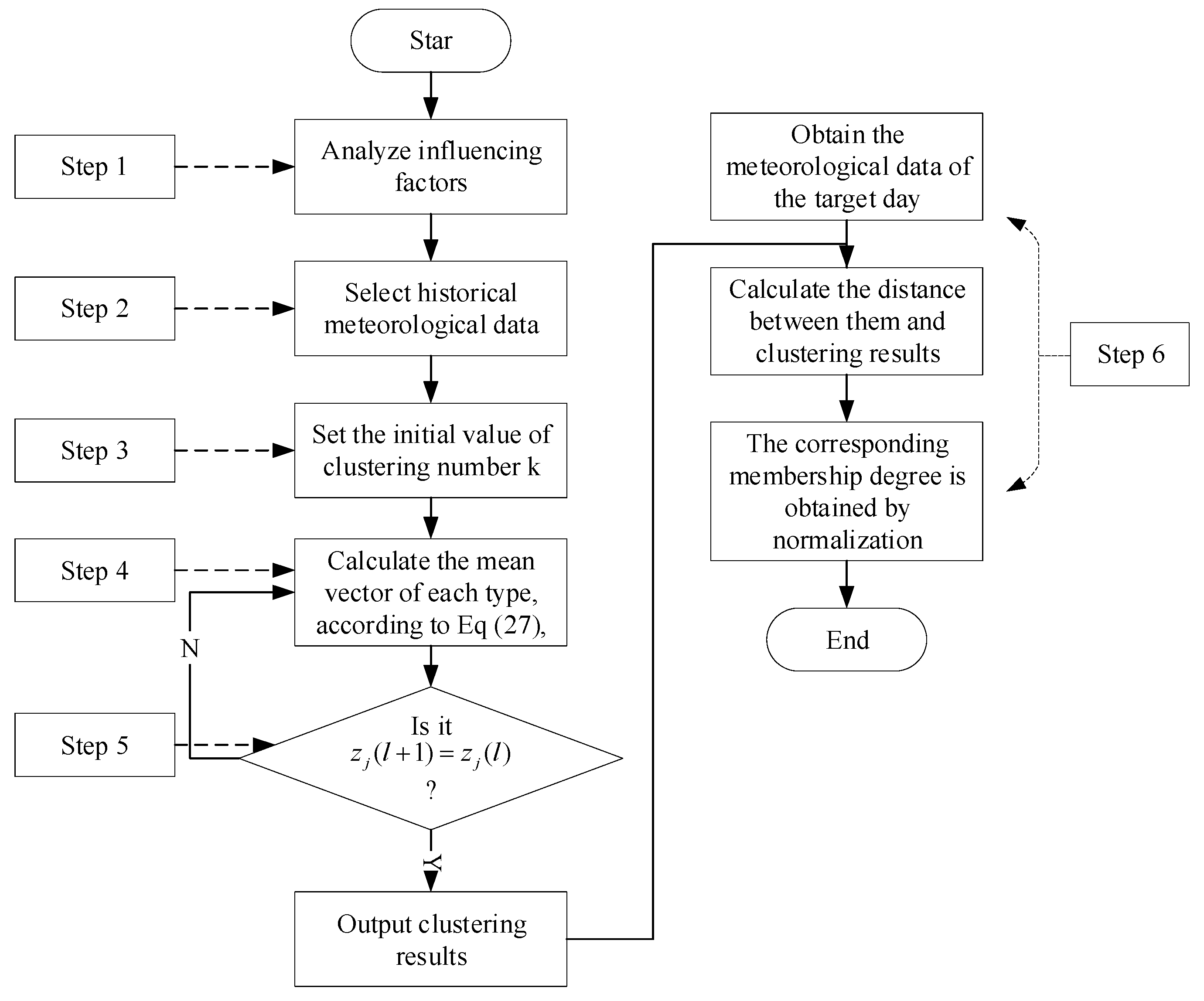
The flow chart of K-means-NWP steps is as shown in Figure 1.

Through Figure 1, we can get n clustering results and the corresponding meteorological data types of each result. As shown in Equation (28),

$$\begin{array}{cc}{K}_1\hfill & =[PavV\min V\max T\min T\max D\sin D\cos ]\\ K_2\hfill & =[PavV\min V\max T\min T\max D\sin D\cos ]\\ K_3\hfill & =[PavV\min V\max T\min T\max D\sin D\cos ]\\ ⋮\hfill & ⋮\\ K_n\hfill & =[PavV\min V\max T\min T\max D\sin D\cos ]\end{array}.$$

(28)

In this paper, in order to simplify the calculation, we take n = 3 to get three scenarios of high, medium, and low wind power output, which is expressed as $\left[K_h;K_m;K_l\right]$, and then calculate the membership degree of the target day meteorological data corresponding to the three scenarios of high, medium and low wind power output, which is expressed as $\left[{\rho }_h,{\rho }_m,{\rho }_l\right]$. Thus, the predictive value of target daily wind power output in each scenario can be obtained.

$$\{\begin{array}{l}{P}_h=[P_1;P_2\dots \dots P_n];\rho ={\rho }_h\\ P_m=[P_1;P_2\dots \dots P_n];\rho ={\rho }_m\\ P_l=[P_1;P_2\dots \dots P_n];\rho ={\rho }_l\end{array}n=1,2,\cdots ,24$$

(29)

3.3. Solution Methodology

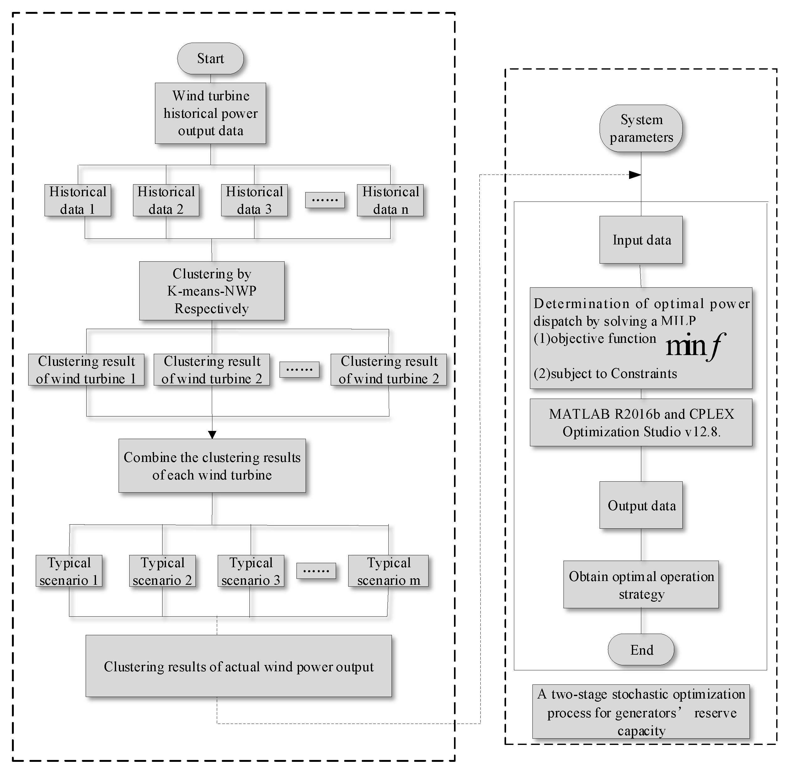
Figure 2 illustrates the solution process of the two-stage stochastic optimization model in this paper. First, the K-means-NWP method is used to cluster the actual output data of each wind turbine, and several possible situations and probabilities of the actual output of wind turbine are obtained. Then, the clustering results of each wind turbine are combined to obtain typical combination scenarios. On this basis, MATLAB R2016b (MathWorks company, Natick, MA, USA, 2016) and CPLEX Optimization Studiov12.8 (IBM company, Amund, New York, NY, USA, 2017) are used to solve the mixed integer linear programming model proposed in Section 3.1, and the unit scheduling results in the day-ahead and real-time phases are obtained. The detailed solution process is shown as follows:

4. Numerical Example

In the numerical example, this paper adopts the basic data of related physical components in the previous literature, and on this basis, the model algorithm proposed in Section 3 is used to realize the simulation, which studies the effect of reserve capacity compensation mechanism on GENCOs’ revenue and quantity of wind spillage. Meanwhile, the impact of changes in related parameters on spare capacity allocation, reserve costs, and wind power consumption is investigated, and the calculated results also meet the expectations, verifying the effectiveness and applicability of the proposed method.

4.1. Parameters Setting

In this section, the power system contained thermal units, wind power generators and interruptible load is set up, and necessary input information and data is presented [29,30]. We build a power system that aggregates four thermal units and two wind turbines. The install capacity of the two wind turbines is 150 MW and 100 MW.

Table 1. The key parameters of generation companies (GENCOs) (Unit: MW, MW/15 min).

GENCOs	Parameters	Value
Thermal Unit 1	$P_{g_1}^{max}$	350
	$P_{g_1}^{min}$	50
	$r_{g_1,u}$	34.5
	$r_{g_1,d}$	34.5
Thermal Unit 2	$P_{g_2}^{max}$	240
	$P_{g_2}^{min}$	50
	$r_{g_2,u}$	67.5
	$r_{g_2,d}$	67.5
Thermal Unit 3	$P_{g_3}^{max}$	200
	$P_{g_3}^{min}$	80
	$r_{g_3,u}$	123
	$r_{g_3,d}$	123
Thermal Unit 4	$P_{g_4}^{max}$	250
	$P_{g_4}^{max}$	50
	$r_{g_4,u}$	69
	$r_{g_4,d}$	69
Wind Turbine 1	$r_{w_1,u}$	34
	$r_{w_1,d}$	34
Wind Turbine 2	$r_{w_2,u}$	22
	$r_{w_1,d}$	22

demonstrates the key parameters of the GENCOs, and

Table 2. The parameters of electricity market.

Parameters	ξ	θ	CS
value	0.2	0.005	800

shows the parameters of electricity market. In addition, we divide spot trading into 96 time periods to simulate scheduling. And the above parameters are substituted into the model, and the model can be solved by Matlab R2016b and CPLEX Optimization Studio v 12.8.

4.2. The Influence of Compensation Mechanism

A two-stage stochastic optimization model proposed in Section 3.1 introduces the reserve capacity compensation mechanism, which provides compensation for the demand response provided by thermal units and the user side. In this section, two different scenarios are set up. By analyzing the operation results of the model, the effect of the introduction of reserve capacity compensation mechanism on wind power consumption and generator revenue is discussed. In order to observe more clearly the influence of compensation mechanism on wind power consumption, the penalty coefficient of wind curtailment is 0 in the two scenarios discussed in this section.

4.2.1. Scenario Set

Case 1

In the traditional power system without reserve capacity compensation mechanism, the total system cost is composed of the operating cost and startup and shut off cost of thermal units. From the perspective of thermal power plants, their revenue is generated by day-ahead dispatching minus operation cost and startup and shut off cost.

$$G={\displaystyle \sum _{t=1}^T{\displaystyle \sum _{g=1}^{N_G}[{\rho }_{g,\mathrm{da}}{P}_g^{Da,t}-(a_i}}{(P_g^{Da,t})}^2+b_i{P}_g^{Da,t}+c_i+{\mu }_g^{t,on}{C}_g^{start}+{\mu }_g^{t,off}{C}_g^{down})]$$

(30)

Case 2

After the reserve capacity compensation mechanism is added into the conventional system, the power plant can obtain the compensation by reserving capacity in the day-ahead market, and meanwhile, the reserve power compensation can be obtained according to the net adjustment amount in the real-time market under the compensation mechanism. In addition to thermal units, the real-time reserve power provided by interruptible load will also obtain compensation. The total system cost increases the reserve capacity cost of thermal units, the compensation cost of calling thermal power plant and the reserve power of interruptible load on the original basis. Similarly, thermal power plants increase the income of reserve capacity and reserve power compensation.

$$\begin{array}{ll}G=& {\displaystyle \sum _{t=1}^T{\displaystyle \sum _{g=1}^{N_G}[{\rho }_{g,\mathrm{da}}{P}_g^{Da,t}+{\rho }_{g,r,u}{R}_g^{t,up,max}+{\rho }_{g,r,d}{R}_g^{t,down,max}+{\rho }_{c,u}{R}_{g,\omega }^{t,up}-{\rho }_{c,d}{R}_{g,\omega }^{t,down}-(a_i}}{(P_g^{Da,t})}^2\\ & +b_i{P}_g^{Da,t}+c_i+{\mu }_g^{t,on}{C}_g^{start}+{\mu }_g^{t,off}{C}_g^{down})]\end{array}$$

(31)

4.2.2. Result and Discussion (High-Medium-Low)

In the day-ahead market, the reserved reserve capacity of thermal units 1–4 and the predicted output of wind turbines 1 and 2 can be obtained according to the calculation results in the first stage of the model, among which the wind power output is the predicted value. According to the clustering method in Section 3.2, the actual output scenarios of wind power are classified as high, medium, and low. The probabilities of each scenario are shown in

Table 3. Clustering results of wind power output.

	High	Medium	Low
wind turbine 1	51.2%	31.5%	17.3%
wind turbine 2	42.4%	29.8%	27.8%

.

Different dispatching results can be obtained under different wind power output combinations. This paper selects five typical combinations—High-High (HH), High-Low (HL), Medium-High (MH), Medium-Medium (MM), and Low-Low (LL). The influence of compensation mechanism on wind power consumption and power generation benefit is analyzed under different wind power output combination.

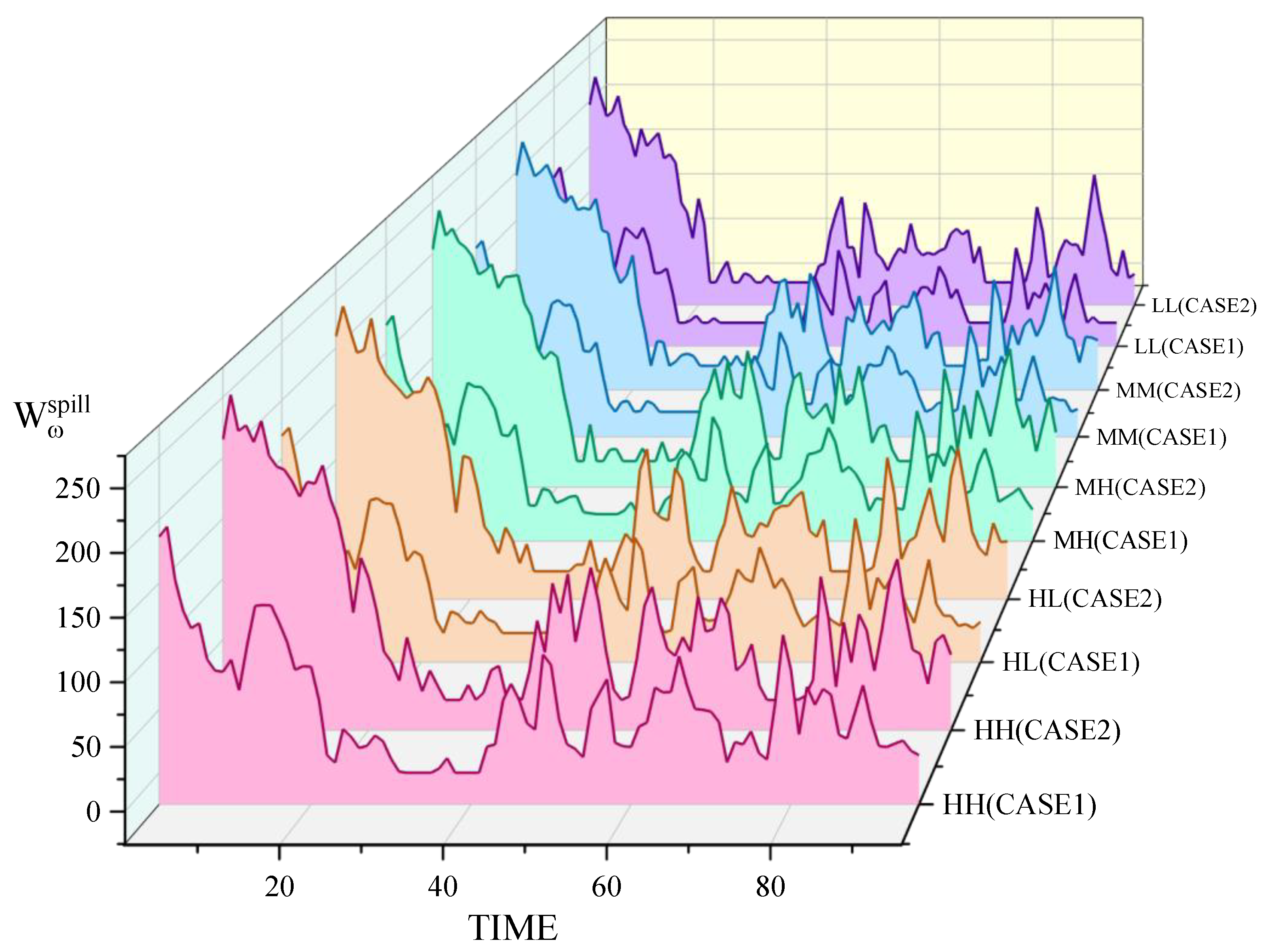
Figure 3 shows the comparison of wind curtailment results in scenario 1 and scenario 2 under different wind power output combinations. It can be seen that the wind curtailment quantity in scenario 1 is significantly less than that in scenario 2, which intuitively illustrates the influence of the reserve capacity compensation mechanism on promoting wind power consumption. In the real-time stage, the thermal unit provides upper reserve capacity $R_{g,\omega }^{t,up}$ and lower reserve capacity $R_{g,\omega }^{t,down}$, while the interruptible load IL provides upper reserve capacity $R_{g,\omega }^{t,IL}$. Then, to promote system balance and wind power consumption, the net reserve power generated in the real-time stage can be expressed as $R_{g,\omega }^{t,down}+R_{g,\omega }^{t,up}+R_{g,\omega }^{t,IL}$. As shown in

Table 4. Each balance unit output under different wind power output combination in the real-time stage during 96 periods.

Wind Power Output Scenario	Case 1			Case 2
	Thermal Unit Down Regulation	Thermal Unit Up Regulation	IL	Thermal Unit Down Regulation	Thermal Unit Up Regulation	IL
HH	1263.55	−125.93	−180.66	4240.83	−11.61	−44.37
HL	859.89	−242.89	−194.71	4128.32	−15.04	−185.94
MH	971.40	−152.99	−186.83	4169.41	−16.54	−258.47
MM	695.67	−138.29	−191.97	4129.06	−27.99	−217.37
LL	702.71	−437.85	−227.80	3966.31	−35.43	−237.69

and Figure 4, when there is a reserve capacity compensation mechanism, thermal units are more active in providing reserve capacity to maintain system balance compared with the net reserve capacity in scenario 1 and scenario 2.

Table 5. Cost-benefit comparison.

Unit: ¥10 Thousand	Case 1	Case 2
Total system cost	411.4	190.4
Power plant revenue:	4087.2	4279.4
Day-ahead generation income	4498.7	4612.9
Capacity of the income	0	341.7
Charge income	0	−230.9
Power generation cost	−411.4	−444.3

demonstrates the composition of the total system cost and the benefits of the power plant under the two scenarios. According to the wind curtailment result in Figure 3, the wind curtailment penalty cost in scenario 2 is also greatly reduced compared with scenario 1 due to the small quantity of wind curtailment. In addition, since scenario 2 absorbs more wind power, and the power generation cost of the wind turbines is 0, its power generation economy is obviously better than that of thermal power units, so the total system cost of scenario 2 is far less than scenario 1. In terms of the income of the GENCOs, the GENCOs in scenario 1 can only obtain the electricity revenue of pre-dispatching in the day-ahead stage. In scenario 2, due to the compensation mechanism of reserve capacity, GENCOs can obtain the compensation of reserve capacity reserved in the day-ahead stage and also gain revenue when the upper reserve power is provided in the real-time stage. Consequently, in scenario 2, the profit of the GENCOs is greatly increased, which can more effectively promote their enthusiasm to provide reserve capacity.

4.3. Impact Factors Analysis on the Wind Power Consumption

From the analysis of Section 4.2, it can be seen that the existence of compensation mechanism in the system is conducive to maintaining the balance of the system and promoting the consumption of the system’s wind power. From the perspective of the GENCOs, the benefits are also increased. This section mainly discusses the influence of the change of relevant parameters in the system on wind power consumption, and the analysis is based on the market with backup capacity compensation mechanism.

In the base scenario, the tariff discount rate is 0.2, the maximum proportion of interruptible load IL in the total load is 0.005, and the penalty coefficient of wind curtailment is 800.

4.3.1. Demand Response Parameters

Figure 5 draws the interruptible load provided by the power side at various time nodes in different wind power scenarios under different tariff discount rates in the real-time stage, As can be seen from Figure 5, in the five different wind power combination scenarios, when $\xi$ = 0.7, the power side provides the most interruptible load to balance the market.

Table 6. Total amount of reserve power provided by interruptible load under different tariff discount rates during 96 time periods.

Tariff Discount Rate	Total Amount of Reserve Power Provided by Interruptible Load (MW)
	HH	HL	MH	MM	LL
0.2	34.09	237.60	214.51	238.50	271.26
0.4	57.96	305.71	279.26	309.88	350.05
0.7	66.74	332.40	293.12	323.96	365.45

illustrates the total amount of interruptible load provided by the power side in one day. Obviously, the interruptible load provided by the power side in the real-time stage will increase with the increase of the tariff discount rate. Compared with the scenario of a low tariff discount rate, the incentive of a high tariff discount rate can promote the power side to make up for the negative error of wind power output to a greater extent. The wind curtailment in various wind power scenarios with different discount rates are illustrated in

Table 7. Total value of wind curtailment at different tariff discount rates during 96 time periods.

Tariff Discount Rate	Total Value of Wind Curtailment (MW)
	HH	HL	MH	MM	LL
0.2	621.13	231.72	462.36	108.39	51.39
0.4	605.80	219.97	455.25	103.70	47.86
0.7	570.42	210.34	427.18	91.87	46.29

. From the perspective of the overall operation of the system, the increase of the tariff discount rate is conducive to wind power consumption and reduce wind curtailment. Figure 6 denotes the pre-output of wind turbines at various time nodes in the day-ahead stage of the system under different tariff discount rates, and the total output of day-ahead wind power under different discount rates is shown in

Table 8. Total pre-output of wind turbines under different tariff discount rates in the day-ahead stage during 96 time periods.

Tariff Discount Rate	The Total Pre-Output of Wind Turbines (MW)
	Wind Turbine 1	Wind Turbine 2	Total
0.2	6599.08	1676.18	8275.26
0.4	6014.50	2290.93	8305.43
0.7	6249.37	2104.43	8353.80

. The increase of tariff discount rate affects the output of units in the equilibrium stage and also changes the pre-output of wind turbines in the day-ahead stage. It can be seen that, as opposed the situation in Section 4.1, with the increase of the tariff discount rate, the pre-output of wind turbines in the day-ahead stage is gradually increased under the condition that the actual output of wind power in the real-time stage is the same, which is equivalent to reducing the pressure of balancing wind power fluctuations in the real-time stage. In this process, the results in

Table 9. Net reserve power at different tariff discount rates during 96 time periods.

Tariff Discount Rate	Net Reserve Power (MW)
	HH	HL	MH	MM	LL
0.2	4178.33	3309.44	3618.84	3193.27	2345.67
0.4	4163.48	3291.03	3595.77	3167.79	2319.03
0.7	4150.50	3252.29	3575.47	3131.25	2272.23

are produced because more wind power has completed pre-dispatching in the day-ahead stage. In addition, with the increase of the tariff discount rate, the net reserve power provided by other units in the real-time phase gradually decreases.

Another parameter that affects the demand response is the interruptible load limit that can be provided by the power side, represented by the proportion of interruptible load to the total load. The system operation results under different $\theta$ values are shown in

Table 10. Total pre-output of wind turbine in different interruptible load limits in day-ahead stage during 96 time periods.

Interruptible Load Limits	Wind Turbine 1	Wind Turbine 2	Total
0.005	6599.08	1676.18	8275.26
0.05	6206.46	2194.97	8401.42
0.1	6474.96	1970.40	8445.36

,

Table 11. Net reserve power under different interruptible load limits during 96 time periods.

Interruptible Load Limits	Net Reserve Power during 96 Time Periods (MW)
	HH	HL	MH	MM	LL
0.005	4799.46	3541.17	4081.19	3301.66	2397.06
0.05	4673.30	3415.01	3955.03	3175.50	2270.90
0.1	4629.36	3371.06	3911.09	3131.55	2226.96

and

Table 12. Total value of wind curtailment under different limits of interruptible load during 96 time periods.

Interruptible Load Limits	Total Value of Wind Curtailment (MW)
	HH	HL	MH	MM	LL
0.005	621.14	231.73	462.36	108.39	51.39
0.05	550.26	219.92	424.00	112.36	48.45
0.1	513.36	183.55	392.49	83.06	42.27

. Similar to the tariff discount rate, with the increase of the $\theta$ value, the wind curtailment quantity in each scenario decreases, and as the output value of pre-dispatch of wind power in the day-ahead stage increases with the increase of the $\theta$ value, the total reserve capacity provided by other units in the real-time stage also decreases.

4.3.2. Penalty Coefficient for Wind Curtailment

The change of penalty coefficient of wind curtailment also has a great influence on the result of the system operation. Different system operation results are obtained when the penalty coefficient of wind curtailment is the various values shown in

Table 13. The range of parameters.

Parameters	Value
$\xi$	0.2	0.4	0.7
$\theta$	0.005	0.05	0.1
$C^S$	800	500	200

. Figure 7 denotes the comparison of wind curtailment curves of the system in one day under different penalty coefficient of wind curtailment. Meanwhile,

Table 14. The total quantity of wind curtailment in each wind power output scenario under different penalty coefficients of wind curtailment during 96 time periods.

Penalty Coefficient of Wind Curtailment	The Total Quantity of Wind Curtailment (MW)
	HH	HL	MH	MM	LL
200	2030.09	1154.49	1455.50	736.86	462.28
500	1168.55	449.70	858.52	211.03	86.49
800	621.13	231.72	462.36	108.39	51.39

demonstrates the sum of wind curtailment quantity in each wind power scene under different penalty coefficient of wind curtailment. It is clear that, in each wind power scenario, the higher the penalty coefficient of wind curtailment, the less the wind curtailment quantity of the system will be. It is obvious that, in the case of a high penalty coefficient of wind curtailment, the system will try to use the reserve capacity of thermal units to absorb wind power in order to reduce the total cost of the system.

Table 15. Net reserve capacity under different penalty coefficients of wind curtailment during 96 time periods.

Penalty Coefficient of Wind Curtailment	Net Reserve Capacity (MW)
	HH	HL	MH	MM	LL
200	4224.72	3842.03	4081.03	4020.14	3390.13
500	4220.84	3681.40	3812.60	3680.56	2900.50
800	4178.33	3309.44	3618.84	3193.27	2345.67

shows the sum of the net reserve capacity provided by the thermal unit and the load side in one day under different penalty coefficient of wind curtailment in the real-time stage. While the penalty coefficient of wind curtailment increases, the sum of net reserve capacity in the real-time stage gradually decreases. This is because, in the case that the actual output value of wind power is the same, the higher the penalty coefficient of wind curtailment, the more pre-dispatch the system will make to wind turbines in the day-ahead stage, as shown in

Table 16. Total pre-output of wind turbines under the penalty coefficient of wind curtailment in the day-ahead stage during 96 time periods.

Penalty Coefficient of Wind Curtailment	The Pre-Output of Wind Turbines (MW)
	Wind Turbine 1	Wind Turbine 2	Total
200	5197.05	1622.86	6819.91
500	6145.76	1539.57	7685.33
800	6599.08	1676.18	8275.26

. should be noted that, compared with the data in Table 9, Table 11, and Table 16, the change of penalty coefficient of wind curtailment has a more significant impact on wind power consumption than the change of wind turbine pre-output caused by the change of relevant parameters of demand response. The change of penalty coefficient of wind curtailment can affect wind power consumption to a greater extent.

5. Conclusions

In this paper, we introduce a reserve capacity compensation mechanism and propose a two-stage stochastic optimization model based on demand response and wind power consumption on the basis of considering the total cost of the day-ahead stage and the real-time stage. Since the actual output of a wind turbine is uncertain, this paper uses K-means-NWP scenario clustering method to process. The wind power output is divided into three scenarios—high, medium, and low—and the actual unit data and market data are used to analyze the system operation result and wind power consumption situation with or without a reserve capacity compensation mechanism and then to compare the influence of different parameters in the system on the wind power consumption result. The conclusions are as follows:

(1) Operating results in a variety of wind power output combination scenarios all prove that after the introduction of reserve capacity compensation mechanism, the system’s wind abandoning capacity is significantly reduced, and thermal units and interruptible loads are also significantly more active in providing reserve capacity, which is conducive to maintaining system balance and promoting wind power consumption.

(2) From the perspective of GENCOs, the reserve capacity compensation mechanism greatly increases the income of GENCOs and thus their enthusiasm to provide reserve capacity. This also plays an active role in promoting wind power consumption, stabilizing wind power output instability, and maintaining system balance.

(3) As the tariff discount rate increases, the power side provides more interruptible load in the balance stage. Compared with the scenario of a low tariff discount rate, the incentive of a high tariff discount rate can promote the power side to stabilize the negative error of wind power output to a greater extent. The increase of the tariff discount rate is helpful for wind power consumption and reduce wind abandoning. Similarly, with the increase of the proportion of the total load of interruptible load stations, the analysis of the system operation results also reached the same conclusion.

(4) The increase of the penalty coefficient of wind curtailment has a great influence on the system operation result. With the increase of the penalty coefficient of wind curtailment, the total wind abandoning quantity of the system is greatly reduced. The higher the penalty coefficient of wind curtailment is, the more pre-dispatching the system will make to the wind turbine in the day-ahead stage. Compared with the change of parameters $\xi$ and $\theta$, the change of $C^S$ has a more significant impact on the wind abandoning quantity and wind power consumption of the whole system.

In conclusion, this paper puts forward targeted suggestions for further promotion of wind power consumption, hoping to provide reference for subsequent research. However, there are other ways to promote wind power consumption such as energy storage. The energy storage system has a response speed of at least minute, and it can store the power in the valley load period and release it in the peak load period. Considering the contribution of an energy storage system in promoting wind power consumption is a worthy subject for further research, which will be further discussed in a future paper. In addition, the construction of the core model is still relatively ideal, which does not consider the blocking effect of the physical power grid in the actual operation process. Future research can be extended in this direction.

References

1. Rahman, M.M.; Velayutham, E. Renewable and non-renewable energy consumption-economic growth nexus: New evidence from South Asia. Renew. Energy 2020, 147, 399–408. [Google Scholar] [CrossRef]
2. DeCastro, M.; Salvador, S.; Gómez-Gesteira, M.; Costoya, X.; Carvalho, D.; Sanz-Larruga, J.F.; Gimeno, L. Europe, China and the United States: Three different approaches to the development of offshore wind energy. Renew. Sustain. Energy Rev. 2019, 109, 55–70. [Google Scholar] [CrossRef]
3. Qi, Y.; Dong, W.; Dong, C.; Huang, C. Understanding institutional barriers for wind curtailment in China. Renew. Sustain. Energy Rev. 2019, 105, 476–486. [Google Scholar] [CrossRef]
4. Edmunds, C.; Martín-Martínez, S.; Browell, J.; Gómez-Lázaro, E.; Galloway, S. On the participation of wind energy in response and reserve markets in Great Britain and Spain. Renew. Sustain. Energy Rev. 2019, 115, 109360. [Google Scholar] [CrossRef]
5. Vogler-Finck, P.J.; Früh, W.G. Evolution of primary frequency control requirements in Great Britain with increasing wind generation. Int. J. Electr. Power Energy Syst. 2015, 73, 377–388. [Google Scholar] [CrossRef]
6. Zhang, Y.; Le, J.; Zheng, F.; Zhang, Y.; Liu, K. Two-stage distributionally robust coordinated scheduling for gas-electricity integrated energy system considering wind power uncertainty and reserve capacity configuration. Renew. Energy 2019, 135, 122–135. [Google Scholar] [CrossRef]
7. Ding, T.; Wu, Z.; Lv, J.; Bie, Z.; Zhang, X. Robust co-optimization to energy and ancillary service joint dispatch considering wind power uncertainties in real-time electricity markets. IEEE Trans. Sustain. Energy 2016, 7, 1547–1557. [Google Scholar] [CrossRef]
8. Fang, X.; Cui, H.; Yuan, H.; Tan, J.; Jiang, T. Distributionally-robust chance constrained and interval optimization for integrated electricity and natural gas systems optimal power flow with wind uncertainties. Appl. Energy 2019, 252, 113420. [Google Scholar] [CrossRef]
9. Yuan, S.; Dai, C.; Guo, A.; Chen, W. A novel multi-objective robust optimization model for unit commitment considering peak load regulation ability and temporal correlation of wind powers. Electr. Power Syst. Res. 2019, 169, 115–123. [Google Scholar] [CrossRef]
10. Zhou, Y.; Wei, Z.; Sun, G.; Cheung, K.W.; Zang, H.; Chen, S. A robust optimization approach for integrated community energy system in energy and ancillary service markets. Energy 2018, 148, 1–15. [Google Scholar] [CrossRef]
11. Hu, D.; Ryan, S.M. Stochastic vs. deterministic scheduling of a combined natural gas and power system with uncertain wind energy. Int. J. Electr. Power Energy Syst. 2019, 108, 303–313. [Google Scholar] [CrossRef]
12. Xu, B.; Zhu, F.; Zhong, P.A.; Chen, J.; Liu, W.; Ma, Y.; Guo, L.; Deng, X. Identifying long-term effects of using hydropower to complement wind power uncertainty through stochastic programming. Appl. Energy 2019, 253, 113535. [Google Scholar] [CrossRef]
13. Zhao, S.; Fang, Y.; Wei, Z. Stochastic optimal dispatch of integrating concentrating solar power plants with wind farms. Int. J. Electr. Power Energy Syst. 2019, 109, 575–583. [Google Scholar] [CrossRef]
14. Yin, Y.; Liu, T.; He, C. Day-ahead stochastic coordinated scheduling for thermal-hydro-wind-photovoltaic systems. Energy 2019, 187, 115944. [Google Scholar] [CrossRef]
15. Hungerford, Z.; Bruce, A.; MacGill, I. The value of flexible load in power systems with high renewable energy penetration. Energy 2019, 188, 115960. [Google Scholar] [CrossRef]
16. Chao, L.; Jun, Y.; Zhi, D.; Jifeng, H.; Mingsong, L. Day-ahead economic dispatch of wind integrated power system considering optimal scheduling of reserve capacity. Energy Procedia 2015, 75, 1044–1051. [Google Scholar] [CrossRef] [Green Version]
17. Najafi, M.; Ehsan, M.; Fotuhi-Firuzabad, M.; Akhavein, A.; Afshar, K. Optimal reserve capacity allocation with consideration of customer reliability requirements. Energy 2010, 35, 3883–3890. [Google Scholar] [CrossRef]
18. Nazari, M.E.; Ardehali, M.M. Ardehali. Optimal bidding strategy for a GENCO in day-ahead energy and spinning reserve markets with considerations for coordinated wind-pumped storage-thermal system and CO2 emission. Energy Strategy Rev. 2019, 6, 100405. [Google Scholar] [CrossRef]
19. Sedighizadeh, M.; Esmaili, M.; Mousavi-Taghiabadi, S.M. Optimal joint energy and reserve scheduling considering frequency dynamics, compressed air energy storage, and wind turbines in an electrical power system. J. Energy Storage 2019, 23, 220–233. [Google Scholar] [CrossRef]
20. Crespo-Vazquez, J.L.; Carrillo, C.; Diaz-Dorado, E.; Martinez-Lorenzo, J.A.; Noor-E-Alam, M. Evaluation of a data driven stochastic approach to optimize the participation of a wind and storage power plant in day-ahead and reserve markets. Energy 2018, 156, 278–291. [Google Scholar] [CrossRef]
21. Hu, J.; Yan, Q.; Li, X.; Jiang, Z.Z.; Kahrl, F.; Lin, J.; Wang, P.A. A cooperative game-based mechanism for allocating ancillary service costs associated with wind power integration in China. Util. Policy 2019, 58, 120–127. [Google Scholar] [CrossRef]
22. Jie, M.; Chaohua, D.; Xuexia, Z.; Zhiyu, W.; Weirong, C.; Yejiang, Y. Dynamic Operation Scenario Reactive Power Optimization Assessment With Large-Scale Wind Farm Integration. IFAC-Pap. 2018, 51, 203–208. [Google Scholar] [CrossRef]
23. He, Z.; Zhou, J.; Sun, N.; Jia, B.; Qin, H. Integrated scheduling of hydro, thermal and wind power with spinning reserve. Energy 2019, 158, 6302–6308. [Google Scholar] [CrossRef]
24. Li, Y.; Miao, S.; Zhang, S.; Yin, B.; Luo, X.; Dooner, M.; Wang, J. Areserve capacity model of AA-CAES for power system optimal joint energy and reserve scheduling. Int. J. Electr. Power Energy Syst. 2019, 104, 279–290. [Google Scholar] [CrossRef]
25. Seddig, K.; Jochem, P.; Fichtner, W. Two-stage stochastic optimization for cost-minimal charging of electric vehicles at public charging stations with photovoltaics. Appl. Energy 2019, 242, 769–781. [Google Scholar] [CrossRef]
26. Ghaljehei, M.; Ahmadian, A.; Golkar, M.A.; Amraee, T.; Elkamel, A. Stochastic SCUC considering compressed air energy storage and wind power generation: A techno-economic approach with static voltage stability analysis. Int. J. Electr. Power Energy Syst. 2018, 100, 489–507. [Google Scholar] [CrossRef]
27. Lynch, M.Á.; Nolan, S.; Devine, M.T.; O’Malley, M. The impacts of demand response participation in capacity markets. Appl. Energy 2019, 250, 444–451. [Google Scholar] [CrossRef] [Green Version]
28. Zhang, J.; Ma, Y.; Zhang, X.; Liu, G. A study on the day-ahead power prediction of wind power plants based on clustering analysis. Zhejiang Electr. Power 2018, 37, 42–46. [Google Scholar]
29. Khaloie, H.; Abdollahi, A.; Shafie-Khah, M.; Siano, P.; Nojavan, S.; Anvari-Moghaddam, A.; Catalão, J.P. Co-optimized bidding strategy of an integrated wind-thermal-photovoltaic system in deregulated electricity market under uncertainties. J. Clean. Prod. 2020, 242, 118434. [Google Scholar] [CrossRef]
30. Basu, M. Multi-region dynamic economic dispatch of solar–wind–hydro–thermal power system incorporating pumped hydro energy storage. Eng. Appl. Artif. Intell. 2019, 86, 182–196. [Google Scholar] [CrossRef]
Figure 1. The flow chart of K-means classification based on numerical weather prediction (K-means-NWP).
Sustainability 11 07171 g001
Figure 2. Two-stage stochastic optimization mode solving process.
Sustainability 11 07171 g002
Figure 3. Daily curtailment curve under different wind power output combination.
Sustainability 11 07171 g003
Figure 4. Each balance unit output under different wind power output combination in the real-time stage 96 periods.
Sustainability 11 07171 g004
Figure 5. The interruptible load provided by each time node under different tariff discount rate in thereal-time stage.
Sustainability 11 07171 g005
Figure 6. Pre-output of wind power units at different time nodes under different tariff discount rates in the day-ahead stage.
Sustainability 11 07171 g006
Figure 7. Wind curtailment curves under different penalty coefficients of wind curtailment.
Sustainability 11 07171 g007