Article

Green-Building-Material Supplier Selection with a Rough-Set-Enhanced Quality Function Deployment

1
Business School, Sichuan University, Chengdu 610064, China
2
Faculty of Computing and Information Technology, King Abdulaziz University, Jeddah 21589, Saudi Arabia
3
Andalusian Research Institute in Data Science and Computational Intelligence (DaSCI), University of Granada, 18071 Granada, Spain
*
Author to whom correspondence should be addressed.
Sustainability 2019, 11(24), 7153; https://doi.org/10.3390/su11247153
Submission received: 10 November 2019 / Revised: 7 December 2019 / Accepted: 9 December 2019 / Published: 13 December 2019

Abstract

:
Building material supplier evaluation and selection is a significant strategic-decision problem for reducing construction costs and ensuring the quality of a residential product. As people are increasingly concerning about the green level of a residential product and the competition in the housing market is becoming increasingly fierce, it becomes important to select a green customer-oriented material supplier for property developers. Quality function deployment (QFD) has been proven to be an effective quality-control technique to take customer voices into consideration. However, the relationship matrix in the QFD technique, as a key to translate customer requirements into technical attributes, was subjectively given by decision-makers in previous studies, which failed to reflect customer requirements accurately. The aim of this study is to put forward a neighborhood-rough-set-based quality function deployment model for a green-building-material supplier selection. The neighborhood rough set, as a nonparametric and flexible data-mining approach, can effectively and objectively determine the core relationships between a variety of factors. A rough number-based aggregation approach is applied to effectively and objectively aggregate the evaluations given by a group of experts. Then, the classical double normalization-based multiple aggregation method, which considers two types of normalization methods, three aggregation models, and a comprehensive score formula, is extended in rough-number form in order to rank the alternatives. Afterward, an attempt is made to evaluate and rank eleven alternative building-material suppliers for a repute property developer in mainland China, and the corresponding comparative and sensitive analyses verify the effectiveness and robustness of the proposed hybrid model.

1. Introduction

Environmental deteriorations have forced public and private sectors to think about environmental and sustainable issues. To protect the environment and promote housing industrialization, many provinces in China, such as Shanghai [1], Hainan [2], and Zhejiang [3], have begun to promote whole-decoration residential houses. Materials account for 40% to 45% of the total cost in typical construction projects [4,5]. Meanwhile, it is well-known that the greenness of a residential product largely depends on the environmental performance of the materials it uses. Owing to the fact that the construction material market in mainland China is not yet well developed, the environmental performance, quality, and price of building materials are varied among suppliers. Hence, an effective and efficient green-building-material supplier selection plays a crucial role in ensuring the green level, quality and controlling the cost of a house. It is especially significant for whole-decoration residential products, as many expensive functional interior fit-out materials are involved in these live-directly products, such as integral kitchen cabinet, closets, and bathroom fixtures.
In recent years, customers are paying more and more attention to the green level of a product and incorporating green factors into their choice of living products. Also, as we all know, the users of the whole-decoration products are not property developers but buyers, and the smooth running of these users’ lives significantly depends on the utilization of the interior fit-out materials’ functions. Therefore, the customer satisfaction is a key factor for the evaluation of these material products. The quick and precise responses to customers’ various demands can help property developers choose a customer-oriented green-material supplier, increase their competitiveness in the increasingly competitive housing market, and further promote their business success. Traditional studies on building-material suppler selection concentrated broadly on relevant supplier selection methods and the economic efficiency of suppliers, without considering the voices of customers or customer requirements (CRs), especially rarely taking into account their environmental requirements. However, for an efficient supply chain management to gain success in business, clearly understanding customer needs is of great importance [6,7]. QFD (quality function deployment) [8,9], as a quality-control technique, has been proved to be an effective technique to take the customer voices into consideration. However, in previous studies related to QFD, the relationship matrix that is key to translate the CRs into TAs (technical attributes, such as product features and engineering characteristics), is subjectively given by decision-makers on the basis of their limited knowledge, which may fail to reflect the CRs accurately. To fill this gap, motivated by Bai and Sarkis [10] and Li et al. [11], we propose a novel method in this study based on the neighborhood rough set theory in order to derive the relationship matrix between CRs and TAs objectively. In the information table, the CRs are taken as the decision attributes, while the TAs and alternatives are regarded as the condition attributes and objects, respectively.
In addition, as the building-material supplier selection is a multi-attribute group decision-making (MAGDM) problem, how to express the judgments of a group and choose an appropriate MAGDM method are critical issues [12,13]. The rough number has proved to be an effective and objective tool in presenting the vagueness of human assessments, while the double normalization-based multiple aggregation (DNMA) method, which considers two types of normalized methods, three aggregation models, and a collective ranking score, is an effective ranking method for massive alternatives. Thus, the presented study develops a rough number-based DNMA method to rank the suppliers, which not only can identify the vagueness brought by the subjective individual judgments of the decision-makers (DMs), but also can deduce a stable ranking result.
The contributions of this study involve three folds:
  • We construct the relationship matrix between CRs and TAs based on the neighborhood rough set, which can help to derive the final weights of the TAs with less subjective factors.
  • We develop an integrated model consisting of QFD technique and rough number-based DNMA method to select the optimal supplier. In this model, the voices of customers are taken into consideration. In addition, the vagueness brought by the DMs’ subjective evaluations is addressed, and a robust ranking result is obtained.
  • A case study of a reputed property developers in China is given to implement the proposed model and guide property developers to a clearer understanding of customer standards. The proposed model can assist DMs to directly identify the attributes that customers are most concerned about and provide a ranking order to all the alternative suppliers.
This paper is organized as follows: Section 2 presents a review on the building-material supplier selection and related methodologies. Section 3 gives the framework of the QFD-based DNMA method for supplier selection. A case study is given in Section 4, and its comparative and sensitive analyses are provided in order to illustrate the reasonability of the proposed method. The paper ends in Section 5 with some concluding remarks.

2. Literature Review and Methodologies

In this section, we first give a short literature review on the building-material supplier selection, and then present the methodologies used in the later presentation. The methodologies of this paper contain the QFD method, neighborhood rough sets theory, and the DNMA method.

2.1. Brief Literature Review on Building-Material Supplier Selection

To ensure the quality and reduce cost in an increasingly competitive global market, supply chain management has proved to be one of the indispensable management methods in the construction industry. The first step to implement supply chain management is supplier choosing. Many scholars have studied the critical role of building-material supplier evaluation in the construction industry. Lam et al. [4] constructed a selection model based on the fuzzy PCA (principal component analysis) for solving the material supplier selection problem from the perspective of property developers. Wang et al. [14] proposed a framework by integrating the building information modeling and geographic information system in order to select a resilient building component supplier. Seth et al. [15] demonstrated the impact of competitive conditions on the supplier evaluation process for construction supply chains. Building-material supplier selection is mainly supported by MAGDM methods, which usually involve three aspects: the identification of evaluation attributes for property developers, the determination of attributes weights, and the ranking method. DMs must make a trade-off between several attributes and adopt proper MAGDM techniques to evaluate a finite set of alternatives. For example, Zolfani et al. [7] adopted a hybrid multi-attribute decision-making model consisting of the AHP (analytic hierarchical process) and the COPRAS-G (complex proportional assessment of alternatives to grey relations) to select a building-material supplier. Eshtehardian et al. [16] investigated the most effective attributes on the supplier selection process by a questionnaire survey and integrated the ANP (analytic network process) with AHP to select appropriate suppliers for construction and civil engineering companies. Safa et al. [5] developed an integrated model for the efficient procurement of construction materials, primarily through the use of the TOPSIS (technique for order preference by similarity to ideal solution) method.
Although there are large numbers of studies on building-material supplier selection, most existing studies were conducted based on the attributes that are determined from the characteristics of construction projects or the needs of property developers. As we know, a building development, especially residential-house development, is to meet the needs of buyers. However, few studies have assessed the performance of building-material suppliers by considering customer requirements.

2.2. The QFD Method

Generally, the QFD is used to address the services plan and new product design challenges to meet better customers’ expectations [11,17,18,19,20]. It is an effective technique to translate CRs into TAs by a relationship matrix called the house of quality (HOQ). The HOQ is a basic structure of QFD and includes CRs, CRs’ importance weights, TAs, and the relationship matrix between CRs and TAs [8]. The first step for constructing an HOQ is the clarification of the CRs so that their voices are well understood. For customers, not all CRs have the same level of importance, so a weighting technique should be adopted to weight the CRs. TAs are associated with CRs. The relationship matrix represents how each CR affects its associated TAs, which contributes to deriving the final importance degrees of the TAs.
In recent years, the extensions and applications of the technique are increasing, including the best computer workstation selection [8], performance evaluation of smart bike-sharing program [9], and strategic supplier evaluation [6,21,22]. Although there are many successful QFD applications on supplier selection, to the best of our knowledge, the relationship matrix that was used to translate the CRs into TAs in the previous studies is subjectively given by DMs based on their limited knowledge, which may fail to respond to customers’ voices accurately.

2.3. The Rough Set Theory

Rough set theory is developed as a nonparametric data-mining approach that can effectively determine the core relationships amongst a variety of factors [23]. It has been widely used for identifying data dependencies, evaluating the importance of attributes, and seeking the minimum subset of attributes [11,24,25,26,27]. Utilizing the ability of rough set theory to identify data dependencies, Li et al. [11] identified the correlation measure matrix corresponding to each CR in QFD to design a washing machine.
In the rough set theory, an information system with decision attributes is called an information table or a decision table. Let I S = U , Q = ( T C ) , V , f be an information table, where U = { A i | i = 1 , 2 , , m } is a set of objects, T = { T j | j = 1 , 2 , , n } is a set of condition attributes, and C = { C 1 , C 2 , , C s } is a set of decision attributes. In general, T C = and each attribute from T C forms a mapping f : U V , where V is the value domain of T and C [27,28]. Each nonempty subset P T determines an indiscernibility relation as R P = { ( A i , A ξ ) U × U | f ( A i , t ˜ ) = f ( A ξ , t ˜ ) , t ˜ P } . The indiscernibility relation R P partitions U into a family of disjoint subsets given by U | R P = { [ A ] P | A U } , where [ A ] P denotes the equivalence class determined by A i with respect to P .
The equivalence relation causes vagueness of the two classes. Rough set theory describes these vague classes through the lower and upper approximations. For any class U ˜ U and P T , the lower approximation of C is presented as R P _ ( U ˜ ) = { [ A ] P | [ A ] P U ˜ } , which is also called the positive region of U ˜ and is denoted alternatively as P O S P ( U ˜ ) . The upper approximation is presented as R P ¯ ( U ˜ ) = { [ A ] P | [ A ] P U ˜ } . U ˜ is called a rough set with respect to P if and only if R P _ ( U ˜ ) R P ¯ ( U ˜ ) , and the objects belonging only to the upper approximation but not to the lower approximation compose the boundary region, which is expressed as R B P ( U ˜ ) = R P ¯ ( U ˜ ) R P _ ( U ˜ ) .
The classical rough set model can only be used to evaluate categorical features. In other words, when introducing a classical rough set to process information, a discrete algorithm is often needed to granulate the data, and then equivalence relations are employed to partition the universe, which inevitably leads to the loss of information. To address this defect, Hu et al. [29,30] introduced a neighborhood rough set model, in which neighborhood relations were used to generate a family of neighborhood granules based on the distance relation of attributes, and then these neighborhood granules were used to approximate decision classes. Neighborhood rough set has more flexibility and expands the boundary dimensions of the classical rough set [10,23]. Bai and Sarkis [10] applied the neighborhood rough set to evaluate environmental performance of green suppliers.
Given an arbitrary object A i U and P ˜ T , the neighborhood δ P ˜ ( A i ) of A i in the attribute space P ˜ is δ P ˜ ( A i ) = { A ξ | A ξ U , Δ P ˜ ( A i , A ξ ) δ } , where Δ is a distance function Δ ( A i , A ξ ) 0 . Δ ( A i , A ξ ) = Δ ( A ξ , A i ) and Δ ( A i , A ξ ) = 0 if and only if A i = A ξ . There are two key factors that define a neighborhood. The distance calculation value and the neighborhood threshold size δ . When δ = 0 , the neighborhood rough set model degenerates to the classical rough set model.
The neighborhood rough set can also be described and generalized by introducing a measure of inclusion [29,30] and dependency degree. Given a neighborhood decision table N S = U , T C , M , A ˜ θ 1 and A ˜ θ 2 are two subsets in U , and then the inclusion degree of A ˜ θ 1 in A ˜ θ 2 is defined as I ( A ˜ θ 1 , A ˜ θ 2 ) = | A ˜ θ 1 A ˜ θ 2 | / | A ˜ θ 1 | , A ˜ θ 1 = , where | * | is the cardinality of a set. Given any subset A ˜ U , the lower and upper sets of A ˜ are N κ _ A ˜ = { A i | I ( δ ( A i ) , A ˜ ) κ , A i U } , N κ ¯ A ˜ = { A i | I ( δ ( A i ) , A ˜ ) 1 κ , A i U } , where 0.5 κ 1 . The model degrades to the classical case if κ = 1 . Then, the dependency degree of C to P ˜ is defined as ϖ P ˜ ( C ) = | P O S P ˜ ( C ) | / | A | , U = , where P O S P ˜ ( C ) is the lower approximation for the decision attributes C and is defined as the union of the lower approximation of each decision class.
It is remarkable that, in rough set theory, attributes are divided into two types: condition attributes and decision attributes. Motivated by Bai and Sarkis [10] and Li et al. [11], in this paper, we propose an improved QFD method based on the rough set theory, where condition attributes are used to reflect property developers’ attributes for building-material suppliers and decision attributes are used to express home buyers’ choices based on their demands or experience. In this way, the voices of customers are considered, not through the subjective judgment of DMs, but through the objective historical consumption data of the customers.

2.4. The DNMA Method

The DNMA method [31] is a recently proposed MAGDM method. To reduce the loss of information, it considers two types of normalized methods and three aggregation models with different functions. Meanwhile, this method further ensures the reliability of the collective ranking by applying a weighted Euclidean distance formula to integrate the subordinate utility values with different ranks. The DNMA method has been successfully applied to solve practical problems, such as the screen of early lung cancer [32].
For an MAGDM problem with a set of alternatives A = U = { A 1 , A 2 , , A m } and a set of attributes, T = { T 1 , T 2 , , T n } with the weight vector W = ( ω 1 , ω 2 , , ω n ) T . The decision-making matrix is denoted as X = ( x i j ) m × n , where x i j is the value of alternative A i attribute T j . The steps of the DNMA method are as follows [31].
Step 1. Normalize the decision matrix. The linear normalization value is
z i j = { | x i j x i j min | / | x i j max x i j min | , for benefit criteria | x i j x i j max | / | x i j max x i j min | , for cost criteria
where x i j max and x i j min refer to the maximum and minimum values of attribute T j , respectively. The vector normalization value is
z i j 1 = { x i j / i = 1 m ( x i j ) 2 , for benefit criteria 1 x i j / i = 1 m ( x i j ) 2 , for cost criteria
Step 2. Compute the subordinate utility values through three different subordinate aggregation models, namely the complete compensatory model (CCM), un-compensatory model (UCM), and incomplete compensatory model (ICM), which are expressed as u ˜ 1 ( A i ) = j = 1 n ω j z i j , u ˜ 2 ( A i ) = max j ω j ( 1 z i j ) , and u ˜ 3 ( A i ) = j ( z i j 1 ) ω j , respectively.
Step 3. Rank the alternatives. The subordinate ranking of alternatives can be listed in descending order, based on the assessment results of the first and third subordinate aggregation models. The results derived from the second subordinate aggregation model can be listed in an ascending order. As a result, by integrating the three different models with a weighted Euclidean distance formula [31], the final ranking can be determined based on an integrated score, which is shown as
S i = φ ( u ˜ 1 ( A i ) i = 1 m ( u ˜ 1 ( A i ) ) 2 ) 2 + ( 1 φ ) ( m r 1 ( A i ) + 1 m ( m + 1 ) / 2 ) 2 φ ( u ˜ 2 ( A i ) i = 1 m ( u ˜ 2 ( A i ) ) 2 ) 2 + ( 1 φ ) ( r 2 ( A i ) m ( m + 1 ) / 2 ) 2 + φ ( u ˜ 3 ( A i ) i = 1 m ( u ˜ 3 ( A i ) ) 2 ) 2 + ( 1 φ ) ( m r 3 ( A i ) + 1 m ( m + 1 ) / 2 ) 2
where φ [ 0 , 1 ] is a parameter to indicate the relative importance between the subordinate ranks and the subordinate utility values. The larger S i is, the better the corresponding alternative will be.

3. The Improved QFD Technique Combined with the Rough Number-Based DNMA Method for Supplier Selection

This section first introduces a rough number-based aggregation method to solve the vagueness brought by the subjective judgments of a group. Then, an improved QFD technique integrating the rough set theory is used to determine the weights of TAs in the building-material supplier selection. Finally, to rank the suppliers, a rough number-based DNMA method is proposed.

3.1. Aggregation Method Based on Rough Numbers

Linguistic variables, originally introduced by Zadeh [33], is an intuitive and flexible way for DMs to express qualitative perceptions, since they are in line with the human way of thinking and reasoning. In this paper, the linguistic scale for qualitative evaluation on attributes are defined as L S 1 = { none = 0.1 , very   low = 1 , low = 2 , fairly   low = 3 , more   or   less   low =   4 , equal = 5 , more   or   less   high = 6 , fairly high = 7 , high = 8 , very   high = 9 , extremely   high = 10 } . Suppose that E = { e q | q = 1 , 2 , , Q } is a set of DMs and the judgment of DM e q for alternative A i on attribute T j is x i j q on the linguistic scale L S 1 . The collective evaluation values of alternative A i on attribute T j can be expressed as x ˜ i j = { x i j q | q = 1 , 2 , , Q } .
As we see, several DMs are involved in the assessment process, and the final decision is made on the basis of the subjective evaluations of DMs. Since variations of individual judgments exist, there must be some vagueness brought by these subjective judgments in the aggregated judgments, thus effectively and objectively aggregating these judgments is critical. Rough number, proposed by Zhai et al. [34], has proved to be an effective and objective tool in presenting the vagueness of information given by the involved DMs [35,36,37]. In this regard, Zhu et al. [35] developed a novel rough number-based VIKOR method to evaluate the design concept alternatives. Pamučar et al. [36] combined rough AHP with rough MABAC (multi-attributive border approximation area comparison) method for evaluating university web pages. Song et al. [37] proposed a rough group AHP and rough group TOPSIS to optimize the design concept evaluation under the subjective environment.
Inspired by these achievements, in this paper, we use a rough number-based approach to obtain the aggregation values of a group. Suppose that y i j is an arbitrary object of x ˜ i j . Then, the lower approximation and upper approximation of x i j q can be defined as follows:
A p r _ ( x i j q ) = { y i j x ˜ i j | y i j x i j q } , A p r ¯ ( x i j q ) = { y i j x ˜ i j | y i j x i j q }
The boundary region of x i j q is obtained as follows:
B n d ( x i j q ) = { y i j x ˜ i j | x i j q y i j } = { y i j x ˜ i j | y i j > x i j q } { y i j x ˜ i j | y i j < x i j q }
Then, x i j q can be represented by a rough number I R ( x i j q ) = [ x i j q l , x i j q u ] , which consists of its corresponding lower limit x i j q l and upper limit x i j q u , where:
x i j q l = y i j A p r _ ( x i j q ) / N l , x i j q u = y i j A p r ¯ ( x i j q ) / N u
with N l and N u being the numbers of objects in A p r _ ( x i j q ) and A p r ¯ ( x i j q ) , respectively.
The interval between the lower limit and upper limit is known as the rough boundary, denoted as follows:
R B ( x i j q ) = x i j q u x i j q l
As a result, the rough sequence I R ( x ˜ i j ) can be denoted as I R ( x ˜ i j ) = { [ x i j 1 l , x i j 1 u ] , [ x i j 2 l , x i j 2 u ] , , [ x i j Q l , x i j Q u ] } , and the aggregated rough value of alternative A i on attribute T j is I R ( x i j ) = [ x i j l , x i j u ] , where
x i j l = ( x i j 1 l + x i j 2 l + L + x i j Q l ) / Q , x i j u = ( x i j 1 u + x i j 2 u + L + x i j Q u ) / Q
The basic operations of two rough numbers I R ( x 11 ) and I R ( x 12 ) are [34] I R ( x 11 ) a = [ x 11 l , x 11 u ] a = [ x 11 l × a , x 11 u × a ] ; I R ( x 11 ) I R ( x 12 ) = [ x 11 l , x 11 u ] [ x 12 l , x 12 u ] = [ x 11 l + x 12 l , x 11 u + x 12 u ] ; and I R ( x 11 ) I R ( x 12 ) = [ x 11 l , x 11 u ] [ x 12 l , x 12 u ] = [ x 11 l × x 12 l , x 11 u × x 12 u ] .

3.2. The Weight Determination of TAs

To select the optimal building-material supplier, first we need to identify CRs and TAs, respectively. The investigation methods (such as interview investigation, questionnaire investigation, and observation investigation) can be adopted to identify the CRs [38], while the TAs can be identified through a comprehensive consideration of the related factors from the material certification system, the special needs of the target company, and the identified CRs. To facilitate the presentation, we assume that there are n identified TAs and s identified CRs.

3.2.1. Deriving the Weights of CRs

In this paper, we use a rough number-based pairwise comparison method [35] to obtain the weights of customer requirements. The procedure of this method is as follows:
Step 1. Construct pairwise comparison matrices with the linguistic scale L S 2 = { equal = 1 , slightly   important = 2 , important = 3 , very   important = 4 , extremely   important = 5 } . Here, a questionnaire is conducted by customer representatives e ^ q ^ to obtain the pairwise comparison matrix. Suppose that Q ^ customer representatives are invited and the comparison matrices are described as:
W C ( q ^ ) = [ 1 a 12 q ^ a 1 s q ^ a 21 q ^ 1 a 2 s q ^ a s 1 q ^ a s 2 q ^ 1 ] ,   for   q ^ = 1 , 2 , , Q ^
where a h k q ^ ( 1 h s , 1 k s , 1 q ^ Q ^ ) is the relative importance of CR h on CR k given by customer representative e ^ q ^ , and s is the number of CRs. To satisfy the consistency, a h k q ^ × a k h q ^ = 1 should be held. All customer representatives’ comparison matrices are presented as:
W ˜ C = [ 1 a ˜ 12 a ˜ 1 s a ˜ 21 1 a ˜ 2 s a ˜ s 1 a ˜ s 2 1 ]
where a ˜ h k = { a ˜ h k 1 , a ˜ h k 2 , , a ˜ h k Q ^ } is the sequence of relative importance of CR h on CR k .
Step 2. Construct the rough comparison matrix. By Equations (1) to (3), the element a ˜ h k in W ˜ C is translated into a rough number, presented as I R ( a h k q ^ ) = [ a h k q ^ l , a h k q ^ u ] , where a h k q ^ l is the lower limit of I R ( a h k q ^ ) , while a h k q ^ u is the upper limit. Then, the rough sequence I R ( a ˜ h k ) can be denoted as I R ( a ˜ h k ) = { [ a h k 1 l , a h k 1 u ] , [ a h k 2 l , a h k 2 u ] , , [ a h k Q ^ l , a h k Q ^ u ] } , and the aggregated rough group sequence I R ( a h k ) = [ a h k l , a h k u ] is obtained with
a h k l = ( a h k 1 l + a h k 2 l + + a h k Q ^ l ) / Q ^ , a h k u = ( a h k 1 u + a h k 2 u + + a h k Q ^ u ) / Q ^
Further, the aggregated rough comparison matrix can be obtained as:
I R ( W c ) = [ [ 1 , 1 ] [ a 12 l , a 12 u ] [ a 1 s l , a 1 s u ] [ a 21 l , a 21 u ] [ 1 , 1 ] [ a 2 s l , a 2 s u ] [ a s 1 l , a s 1 u ] [ a s 2 l , a s 2 u ] [ 1 , 1 ] ]
Step 3. Calculate the rough weight I R ( w ˜ C h ) = [ w ˜ C h l , w ˜ C h u ] for each attribute with
w ˜ C h l = k = 1 s a h k l s ,   w ˜ C h u = k = 1 s a h k u s
Finally, we obtain the rough weight vector of customer needs as I R ( w ˜ C ) = ( [ w ˜ C 1 l , w ˜ C 1 u ] , , [ w ˜ C h l , w ˜ C h u ] , , [ w ˜ C s l , w ˜ C s u ] ) T .

3.2.2. Establishing the Relationship of CRs and TAs

In the traditional QFD, the determination of the relationship matrix relies on the experience of DMs. To overcome the inaccuracy caused by this subjective way, we introduce the dependency degree in neighborhood rough set theory, combined with rough numbers, as the relationship measure between CRs and TAs. The CRs and TAs are expressed as C s and T j , respectively. The calculation steps are as follows:
Step 1. Normalize the aggregated rough value of alternative A i on attribute T j as I R ( z i j ) = [ z i j l , z i j u ] . The normalization process is done to establish the same scale for all attributes for the purpose of comparability. Here, we adopt the linear normalization as:
z i j l = { | x i j l x i j min | / | x i j max x i j min | , for   benefit   criteria | x i j u x i j max | / | x i j max x i j min | , for   cost   criteria z i j u = { | x i j u x i j min | / | x i j max x i j min | , for   benefit   criteria | x i j l x i j max | / | x i j max x i j min | , for   cost   criteria
where x i j l and x i j u are the upper and lower limit of the aggregated rough evaluation values for supplier A i on attribute T j , respectively; and x i j max and x i j min are the maximum and minimum values in L S 1 , respectively.
Step 2. Develop the neighborhood decision system based on interval rough numbers. The data is presented in the form of an information system in rough set analysis, with its rows corresponding to objects and its columns corresponding to condition attributes [34]. To construct a neighborhood information system, we should reformat the decision matrix of the supplier evaluation.
In reality, due to the limitation of professional level, when a customer is asked to provide his/her requirements, the opinions are usually somewhat general; that is to say, one CR is based on a set of detailed attributes. For example, when choosing a building-material supplier and customers only consider the environmental protection level, they may not be careful to examine that the general attribute can be reflected in the environmental certification, recycling of materials, etc. However, property developers with certain professional abilities need to consider more-detailed indicators. Therefore, for one C h of the identified CRs, we can always find multiple corresponding TAS. Assume that each C h is independent and a neighborhood information table contains only one decision attribute. In this way, each C h with its associated T C h = { T C h η | η = 1 , 2 , , η # } forms an information system (Table 1), where the candidate building-material suppliers are the objects, and the CRs with their associated TAs are decision attributes and condition attributes, respectively. The number of CRs determines the number of the neighborhood information systems.
In Table 1, the value of decision attribute C h is assigned based on customers’ consumption preferences. Value “1” indicates that customers are unsatisfied with the supplier’s performance under the decision attribute, which means that customers do not select the supplier most of the time. Value “2” indicates a better customer satisfaction, which means customers always choose the supplier under the decision attribute.
Step 3. Compute neighborhood relational matrices for the performance measures. Neighborhood relations are used to group sets of suppliers (objects) based on similarity or indistinguishability, using the neighborhood distance parameter [10]. First, we need to calculate the distances between the suppliers on each T C h η , which result in n m × m distance matrices. Then, we use the Euclidean distance formula to obtain the matrices, which is denoted as follows:
Δ { I R ( z T C h η , i ) , I R ( z T C h η , i 1 ) } = [ ( z T C h η , i l z T C h η , i 1 l ) 2 + ( z T C h η , i u z T C h η , i 1 u ) 2 ] 1 / 2
where I R ( z T C h η , i ) ( 1 i m ) and R ( z T C h η , i 1 ) ( 1 i 1 m ) are the normalized aggregated rough value of T C h η .
Step 4. Determine the neighborhood relation for each performance measure. Here, we need to arrive at a relational matrix R ( T C h ) , which is defined as R ( T C h η ) = ( r i , i 1 ) m × m , with
r i , i 1 = { 1 , Δ { I R ( z T C h η , i ) , I R ( z T C h η , i 1 ) } δ 0 , otherwise
where δ is the neighborhood distance parameter.
Step 5. Determine the inclusion measure and lower rough sets for each CR. We first compute the neighborhood information granule δ T C h η ( A i ) for supplier A i under T C h η with
δ T C h η ( A i ) = i 1 = 1 m r i , i 1
Then, we calculate the relational matrix for the neighborhood suppliers who have the same CR score, and populate the matrix R ( C h ) with
R ( C h ) = ( r ˜ i , i 1 ) m × m ,   r ˜ i , i 1 = { 1 , Δ { I R ( z T C h η , i ) , I R ( z T C h η , i 1 ) } δ , C h , i = C h , i 1 0 , otherwise
Next, we determine the neighborhood information granule δ T C h η C h ( A i ) for a given supplier A i under T C h η and C h :
δ T C h η C h ( A i ) = i 1 = 1 m r ˜ i , i 1
The inclusion measure can be obtained as follows:
I { δ T h η C h ( A i ) , δ T h η ( A i ) } = δ T h η C h ( A i ) / δ T h η ( A i )
We should set a threshold κ to identify the lower rough sets of C h on T C h η . If I { δ T C h η C h ( A i ) , δ T C h η ( A i ) } κ , we say that A i P O S T C h η ( C h ) , which means that supplier A i belongs to the lower neighborhood rough set based on T C h η and C h .
Step 6. Compute the dependency degrees for each CR with its associated TAs. The dependency degree of T C h η to C h is calculated as follows:
ϖ T C h η ( C h ) = | P O S T C h η ( C h ) | / | m |
On the basis of the dependency degree, the relationship between CRS and TAS can be established objectively.

3.2.3. Determine the Final Weights of TAs

The development of residential house is to meet the customers’ needs for life. Quick and precise responses to customers’ various demands can improve the supply chain management and guarantee success in business. In this paper, we consider customer voices by adjusting the weights of attributes given by DMs.
First, property developers are invited to evaluate the initial relative importance of TAs from their technique perspectives. Same as the weighting technique of CRs, the rough set-based pairwise comparison method is applied. The initial rough weight vector of TAs is denoted as I R ( w ˜ ) = ( [ w ˜ 1 l , w ˜ 1 u ] , , [ w ˜ j l , w ˜ j u ] , , [ w ˜ n l , w ˜ n u ] ) T , and the normalized initial weight of a TA is I R ( w j ) = [ w j l , w j u ] with
w j l = min { w j l / j = 1 n w j l , w j u / j = 1 n w j u } , w j u = max { w j l / j = 1 n w j l , w j u / j = 1 n w j u }
Then, based on the dependency degree, the weight of customer to T j ( I R ( w ˜ j , C T ) ) can be obtained by
ϖ j × [ w ˜ C h l , w ˜ C h u ] = [ w ˜ j , C T l , w ˜ j , C T u ]
where ϖ j refers to the dependency degree of C h to T j , [ w ˜ C h l , w ˜ C h u ] is the obtained rough weight vector of C h in Section 3.2.1, and the normalized weight of customer to T j , I R ( w j , C T ) = [ w j , C T l , w j , C T u ] is obtained with
w j , C T l = min { w j , C T l / j = 1 n w j , C T l , w j , C T u / j = 1 n w j , C T u } , w j , C T u = max { w j , C T l / j = 1 n w j , C T l , w j , C T u / j = 1 n w j , C T u }
Afterward, the final weight of a TA can be obtained as follows:
I R ( w ^ j ) = λ I R ( w j , C T ) + ( 1 λ ) I R ( w j ) = [ w ^ l j , w ^ u j ]
where I R ( w j , C T ) refers to the normalized rough weight of customer to T j , while I R ( w j ) refers to the normalized rough weight of initial T j . λ is a parameter which depends on the importance degree of DMs for customer requirements.

3.3. Ranking the Suppliers with the Rough Number-Based DNMA Method

In MAGDM methods, several DMs are involved in the assessment process, and the final decision is made on the basis of the subjective evaluations of DMs. To represent the vagueness brought by the subjective individual assessments, in this paper, a rough set-based DNMA method is developed and then combined with the improved QFD, to select the optimal building-material supplier under a clear and object understanding of customer voices. The steps of the rough set-based DNMA method are as follows.
Step 1. Calculate the linear normalization value I R ( z i j ) = [ z i j l , z i j u ] by Equation (8) and the vector normalization value I R ( z i j 1 ) = [ z i j 1 l , z i j 1 u ] by Equation (20):
z i j 1 l = { min { x i j l / i = 1 m ( x i j l ) 2 , x i j u / i = 1 m ( x i j u ) 2 } min { 1 x i j l / i = 1 m ( x i j l ) 2 , 1 x i j u / i = 1 m ( x i j u ) 2 } ,   z i j 1 u = { max { x i j l / i = 1 m ( x i j l ) 2 , x i j u / i = 1 m ( x i j u ) 2 } max { 1 x i j l / i = 1 m ( x i j l ) 2 , 1 x i j u / i = 1 m ( x i j u ) 2 }
where x i j l and x i j u are the upper and lower limits of the aggregated rough evaluation value for supplier A i on attribute T j .
Step 2. Compute the subordinate utility values through three different subordinate aggregation models. The complete compensatory model (CCM) is expressed as I R { u ˜ 1 ( A i ) } = [ u ˜ 1 l ( A i ) , u ˜ 1 u ( A i ) ] with
u ˜ 1 l ( A i ) = j = 1 n ( w ^ l j × z i j l ) , u ˜ 1 u ( A i ) = j = 1 n ( w ^ u j × z i j u )
The un-compensatory model (UCM) is expressed as I R { u ˜ 2 ( a i ) } = [ u ˜ 2 l ( A i ) , u ˜ 2 u ( A i ) ] with
u ˜ 2 l ( A i ) = max j { w ^ l j × ( 1 z i j l ) } , u ˜ 2 u ( A i ) = max j { w ^ u j × ( 1 z i j u ) }
The incomplete compensatory model (ICM) is expressed as I R { u 3 ( a i ) } = [ u 3 l ( A i ) , u 3 u ( A i ) ] with
u ˜ 3 l ( A i ) = j ( z i j 1 u ) w ^ u j , u ˜ 3 u ( A i ) = j ( z i j 1 l ) w ^ l j
Step 3. Rank the suppliers. The larger the final integrated score of S i = [ S i l , S i u ] is, the better the corresponding alternative will be. S i l = min { S ˜ i l , S ˜ i u } , S i u = max { S ˜ i l , S ˜ i u } (for i = 1 , 2 , , m ) are calculated by Equation (24), and the comparison rules of rough numbers (please refer to [34]) are used to obtain the ranking results.
S ˜ i l = φ ( u ˜ 1 l ( A i ) i = 1 m ( u ˜ 1 l ( A i ) ) 2 ) 2 + ( 1 φ ) ( m r 1 ( A i ) + 1 m ( m + 1 ) / 2 ) 2 φ ( u ˜ 2 l ( A i ) i = 1 m ( u ˜ 2 l ( A i ) ) 2 ) 2 + ( 1 φ ) ( r 2 ( A i ) m ( m + 1 ) / 2 ) 2 + φ ( u ˜ 3 l ( A i ) i = 1 m ( u ˜ 3 l ( A i ) ) 2 ) 2 + ( 1 φ ) ( m r 3 ( A i ) + 1 m ( m + 1 ) / 2 ) 2 , S ˜ i u = φ ( u ˜ 1 u ( A i ) i = 1 m ( u ˜ 1 u ( A i ) ) 2 ) 2 + ( 1 φ ) ( m r 1 ( A i ) + 1 m ( m + 1 ) / 2 ) 2 φ ( u ˜ 2 u ( A i ) i = 1 m ( u ˜ 2 u ( A i ) ) 2 ) 2 + ( 1 φ ) ( r 2 ( A i ) m ( m + 1 ) / 2 ) 2 + φ ( u ˜ 3 u ( A i ) i = 1 m ( u ˜ 3 u ( A i ) ) 2 ) 2 + ( 1 φ ) ( m r 3 ( A i ) + 1 m ( m + 1 ) / 2 ) 2

4. Case Study

To illustrate the validity and efficiency of the proposed QFD-based DNMA method with rough numbers, in this section, we make an attempt to evaluate and rank eleven alternative building-material suppliers for a reputable property developer in China. To verify the effectiveness and the robustness of the proposed model, comparative and sensitive analyses are conducted.

4.1. Case Description

The construction of whole-decoration residential products involves hundreds of building materials, such as brick, concrete, emulsion paint, integral kitchen cabinet fixture, and bathroom fixtures. In the fit-out phase, the green level, quality, and price of some functional materials vary among suppliers, and the material-supplier selection will affect the customers’ purchase intention of a whole-decoration residential product. Integral kitchen cabinet is one of the most important functional fit-out materials. On one hand, its expense accounts for a large proportion of the overall fit-out cost, and it is important in quality guarantee of a residential product; on the other hand, people use it every day for their three meals, which determines the importance of this material to home buyers. Thus, this study takes the integral-kitchen-cabinet supplier selection as an example.
Company A is one of the largest and most comprehensive property developers in China. In 2009, the property developer announced its residential whole-decoration strategy, and up to now, more than 80% of its residential products delivered to customers have been achieved in whole-decoration. To improve the green level and the quality of their delivered residential products, and reduce the cost of product fit-out through supply chain management, the management committee of the property developer conducts supplier decisions by using MAGDM methods. Eleven integral-kitchen-cabinet suppliers were selected from their supplier list for the case study.

4.2. Implementation

To investigate customer requirements and ratings of integral-kitchen-cabinet suppliers for a whole-decoration residential product, the interview survey method, combined with the questionnaire survey method, was adopted.
First, by interviewing real estate enterprises’ target customers and sales staff, we found that, for an integral kitchen cabinet of a residential product, customers are most concerned about the economic performance, the environmental certification, and the market performance. Then, 1000 questionnaires were distributed to five buildings’ sales halls, to collect the ratings of the integral-kitchen-cabinet suppliers from residential products’ visitors/buyers. The ratings should be given according to these target customers’ historical experiences, and the rating levels are divided into two: “2” for always choosing and choosing with high probability; “1” for hardly choosing and never choosing. If more than 60% of customers choose “2”, we give the supplier a rating of “2”; otherwise, a rating of “1” is given. The results are shown in Table 2 by sorting out and analyzing the collected questionnaires.
Then, a decision-making group is invited to determine the TAs based on the material certification system, the special needs of their company, and the identified customer requirements. For example, since the company A focuses on the long-term relationship with the selected supplier, so as to deliver the residential products better, faster, and smoother, the cooperation willingness is defined as a TA. The TAs are shown in Table 3.
The decision-making group consists of five members { e 1 , e 2 , e 3 , e 4 , e 5 } : the chief executive e 1 , the general manager e 2 , the contract management manager e 3 , and two experts e 4 , e 5 with a minimum of five years of experience managing a supply chain in a real-estate development company. The decision-making group is required to provide their individual evaluations on the 11 candidates on each TA (shown in Table 4). After that, we use the rough number-based approach to aggregate individual DMs’ judgments, and the results are listed in Table 5.
Next, we derive the final weights of TAs in three phases:
Phase 1 is to derive the weights of CRs. Ten customer representatives are invited to give their pairwise comparisons of the CRs (shown in Table 6). Based on Equations (1) to (3), the rough comparison values are obtained, shown in (Table 7). Then, the rough weights of CRs are obtained by Equations (6) to (7) as I R ( w ˜ C ) = { [ 0.98 , 1.22 ] , [ 1.04 , 1.27 ] , [ 0.78 , 0.96 ] } .
Phase 2 is to establish relationships between CRs and TAs. First, we should normalize the collective rough values of the DMs (shown in Table 8). Then, we should find a set of corresponding TAS for each C h . Since the identified CRs are independent, each C h with its associated T C h could form an information system. In this case study, three information tables are constructed. According to DMs’ opinions, T 1 T 4 are related to C 1 , and T 5 T 7 are related to C 2 , while T 8 T 12 are related to C 3 . We set δ = 0.1 and κ = 0.8 . Here we display the calculation processes only for the second attribute T 2 that relates to C 1 , denoted as T C 1 2 . Table 9 shows the information system that takes C 1 as the decision condition. By Equations (9) to (11), the neighborhood relations and neighborhood information granule for supplier A i on T C 1 2 ( δ T C 1 2 ( A i ) ) can be computed (shown in Table 10). Next, using Equations (12) to (14), the inclusion degrees of T C 1 2 are obtained as I { δ T C 1 2 C 1 ( A i ) , δ T C 1 2 ( A i ) } = { 1 , 0.5 , 0.67 , 1 , 1 , 0.67 , 1 , 1 , 0.33 , 1 , 0.5 } . All the results are listed in Table 11. When κ is set as 0.8, we get the lower rough sets P O S T C 1 η ( C 1 ) of C 1 to T 2 as { A 1 , A 4 , A 5 , A 7 , A 8 , A 10 } . Finally, the dependency degree of C 1 to T 2 is obtained as 0.55 by Equation (15). By repeating the above steps, we can acquire the objective relationships between CRs and TAs, which are presented in Table 12.
From the yield results, we can see that customers are highly dependent on attributes T 1 , T 4 , T 5 , T 7 , T 9 and T 10 , while they pay less attention to attributes T 3 , T 8 and T 11 . In other words, customers are especially concerned about the green level, quality, and service of an integral kitchen cabinet product. Meanwhile, we can also see that, comparing with price, customers pay more attention to the product’s quality.
Phase 3 is to determine the final weights of TAs. Each weight consists of two parts: the weight of customer to T j ( I R ( w ˜ j , C T ) ) and the weight given by property developers’ DMs ( I R ( w j ) ) which is also called the initial relative importance of TAs. The same as CRs, we acquire the initial weights of TAs through the rough number-based pairwise comparison method. Since there are 12 TAs, according to the AHP method, a stratification is needed for weighting these attributes. In our illustrated case study, we exploit the relationships with CRs to stratify the TAs. The interlevel calculation process can be found in [39]. By applying Equations (16) to (19), the final weights of TAs that customer voices are taken into accounts were derived, shown in Table 13, where the parameter λ is set as 0.4.
After acquiring the final weights of TAs, we then rank the suppliers by the rough set-based DNMA method. First, we normalize the aggregated rough judgments. The linear normalized values were calculated in Table 8, while the vector normalized values can be computed by Equation (20) (shown in Table 14). Then, Equations (21) to (24) and the comparison rules of rough numbers [34] are employed to determine the final ranking of the alternatives with φ = 0.5 . The results are shown in Table 15. The comprehensive ranking of the alternatives is A 3 > A 11 > A 7 > A 6 > A 2 > A 9 > A 10 > A 4 > A 8 > A 5 > A 1 , where A 3 is supposed to be the optimal suppliers considering the voices of customers.

4.3. Comparison and Discussion

To verify the effectiveness and robustness of the proposed approach in this paper, comparative and sensitive analyses are conducted in this subsection.
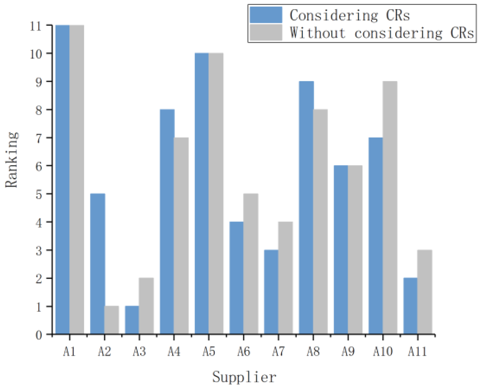
We first compare the results after and before considering customer needs. The results yielded by the rough DNMA method are shown in Figure 1, through which we find that, when customer voices are taken into accounts, supplier A 3 is believed to be the optimal suppliers, while when evaluating these suppliers only from the perspective of the property developer, supplier A 2 is the best one. With the in-depth analysis on Table 2, we find that supplier A 3 offers a good customer experience, since its integral kitchen cabinet products are always in the choice lists of customers, while that of supplier A 2 is relatively poor, given that the supplier gains poor ratings from customers, both in the aspects of economic performance and environmental certification. From this analysis, we can see that our method effectively takes the customer voices into consideration.
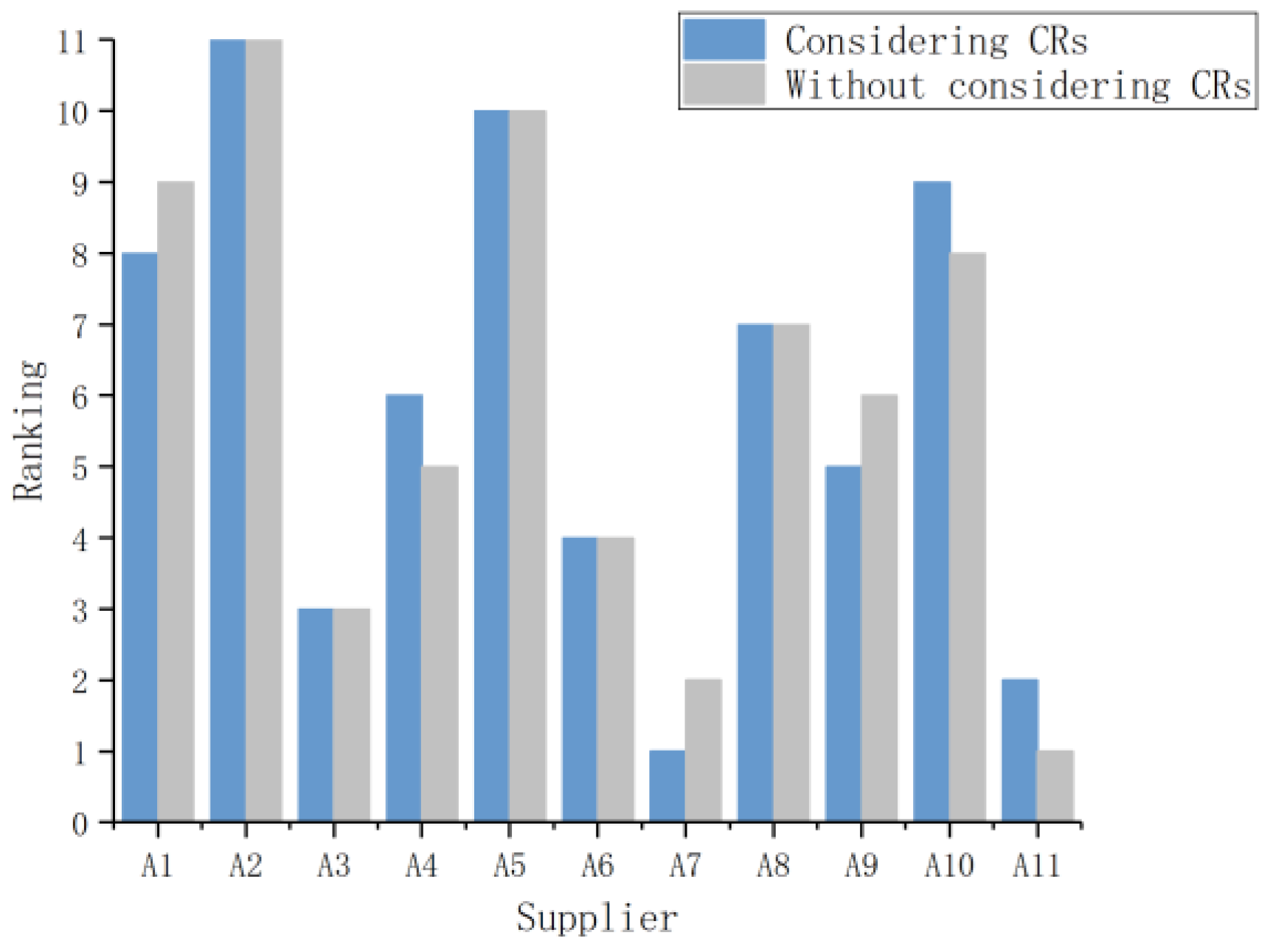
In the second comparative analysis, we integrate our improved QFD method with the rough VIKOR method [35], to verify the effectiveness of our method. The results are illustrated in Figure 2. From this figure, we can find similar results. Supplier A 11 is the recommend one before considering customer needs, but the supplier’s ratings by customers are poor in the aspect of market performance. Supplier A 7 is the best choice after considering customer voices, which matches the ratings of the customer to suppliers. Therefore, customer voices were successfully considered in our proposed approach.
In the case study, we set two important parameters that relate to the neighborhood rough set as δ = 0.1 and κ = 0.8 . The setting of the two parameters may affect the dependency degrees of CRs to TAs. Therefore, it is necessary to verify the robustness of the model through sensitive analysis. Here, the parameter δ is set as 0 δ 0.2 , and κ is set as 0.8 κ 1 , of which the increment is 0.05. Twenty-five tests are conducted. The results yielded are shown in Figure 3, through which we can see A 3 is always the optimal supplier and A 11 is always the last one. The top-five rakings generated are A 2 , A 3 , A 6 , A 7 and A 11 . Overall, the results of the 25 tests are with small fluctuation in a normal range, which indicates the robustness of our proposed method.
5. Conclusions

The whole-decoration residential house has become the main form of residential products in the current Chinese housing market. The construction of these live-directly products involves many interior functional fit-out materials. On the one hand, materials account for nearly half of the total cost in construction, and the green level of a residential product closely related to the environmental performance of its building materials; on the other hand, customer satisfaction of material and its suppliers, especially of these interior functional fit-out materials, is of great importance for the success sells of the residential products. Thus, a framework should be established to comprehensively evaluate the performance of building-material suppliers and help property developers select a green customer-oriented supplier. This study constructed a multiphase QFD-based decision framework for the selection of the optimal building-material suppliers, by taking into account customers’ voices. Compared with the supplier evaluations in previous QFD studies, the proposed framework constructed the relationship matrix between CRs and TAs based on the neighborhood rough set theory, which can respond to customers’ voices more objectively. Then, the ranking method of rough number-based DNMA method, which considered two types of normalization methods, three aggregation models, and a comprehensive score function by integrating the subordinate utility values with their ranks, was employed to determine the ranking of alternatives. Finally, comparative analysis was conducted both before and after considering CRs in the rough set-based DNMA method. The corresponding results showed that the proposed approach effectively took the customers’ voices into consideration, and the similar results were found in the rough set-based VIKOR method. Moreover, a sensitivity analysis was conducted by changing the parameters related to the neighborhood rough set. The result further validated the reasonability and robustness of the proposed approach.
Of course, our studies also have certain limitations that present opportunities for further study. The number of the attributes and candidate suppliers can be increased to provide more comprehensive and accurate research results than the current study. Besides, the hesitant fuzzy linguistic term set [40] can be incorporated into the proposed framework to tackle the inaccurate and fuzzy judgments of DMs, which will be an interesting research topic for a future study.

Author Contributions

Z.Z. and H.L. proposed the original idea and conceived of the study; Z.Z., H.L. and J.C. were responsible for developing the method and collecting and analyzing the data; Z.Z., H.L. and J.C. wrote the first draft of the article; A.A.-b. revised the paper.

Acknowledgments

The work was supported by the National Natural Science Foundation of China under Grant 71771156, 71971145.

Conflicts of Interest

The authors declare no conflicts of interest.

References

  1. The Promotion of Residential Whole-Decoration Strategy in Shanghai. The Central People’s Government of the People’s Republic of China. 2 October 2012. Available online: http://www.gov.cn/jrzg/2012-10/02/content_2237316.htm (accessed on 7 December 2019).
  2. The Promotion of Residential Whole-Decoration Strategy in Hainan. The Central People’s Government of the People’s Republic of China. 23 May 2017. Available online: http://www.gov.cn/xinwen/2017-05/23/content_5196084.htm (accessed on 7 December 2019).
  3. The Promotion of Residential Whole-Decoration Strategy in Zhejiang. The Central People’s Government of the People’s Republic of China. 2 February 2017. Available online: http://www.gov.cn/xinwen/2017-02/02/content_5164705.htm (accessed on 7 December 2019).
  4. Lam, K.C.; Tao, R.; Lam, C.K. A material supplier selection model for property developers using Fuzzy Principal Component Analysis. Autom. Constr. 2010, 19, 608–618. [Google Scholar] [CrossRef]
  5. Safa, M.; Shahi, A.; Haas, C.T.; Hipel, K.W. Supplier selection process in an integrated construction materials management model. Autom. Constr. 2014, 48, 64–73. [Google Scholar] [CrossRef]
  6. Yazdani, M.; Chatterjee, P.; Zavadskas, E.K.; Zolfani, S.H. Integrated QFD-MCDM framework for green supplier selection. J. Clean. Prod. 2017, 142, 3728–3740. [Google Scholar] [CrossRef]
  7. Zolfani, S.H.; Chen, I.S.; Rezaeiniya, N.; Tamošaitienė, J. A hybrid MCDM model encompassing AHP and COPRAS-G methods for selecting company supplier in Iran. Technol. Econ. Dev. Econ. 2012, 18, 529–543. [Google Scholar] [CrossRef] [Green Version]
  8. Onar, S.Ç.; Büyüközkan, G.; Öztayşi, B.; Kahraman, C. A new hesitant fuzzy QFD approach: An application to computer workstation selection. Appl. Soft Comput. 2016, 46, 1–16. [Google Scholar] [CrossRef]
  9. Tian, Z.P.; Wang, J.Q.; Wang, J.; Zhang, H.Y. A multi-phase QFD-based hybrid fuzzy MCDM approach for performance evaluation: A case of smart bike-sharing programs in Changsha. J. Clean. Prod. 2018, 171, 1068–1083. [Google Scholar] [CrossRef]
  10. Bai, C.G.; Sarkis, J. Evaluating supplier development programs with a grey based rough set methodology. Expert Syst. Appl. 2011, 38, 13505–13517. [Google Scholar] [CrossRef]
  11. Li, Y.L.; Tang, J.F.; Chin, K.S.; Han, Y.; Luo, X.G. A rough set approach for estimating correlation measures in quality function deployment. Inf. Sci. 2012, 189, 126–142. [Google Scholar] [CrossRef]
  12. Schotten, P.C.; Morais, D.C. A group decision model for credit granting in the financial market. Financ. Innov. 2019, 5, 6. [Google Scholar] [CrossRef] [Green Version]
  13. Wu, W.S.; Kou, G. A group consensus model for evaluating real estate investment alternatives. Financ. Innov. 2016, 2, 8. [Google Scholar] [CrossRef] [Green Version]
  14. Wang, T.K.; Zhang, Q.; Chong, H.Y.; Wang, X.Y. Integrated supplier selection framework in a resilient construction supply chain: An approach via analytic hierarchy process (AHP) and grey relational analysis (GRA). Sustainability 2017, 9, 289. [Google Scholar] [CrossRef] [Green Version]
  15. Seth, D.; Nemani, V.K.; Pokharel, S.; Al Sayed, A.Y. Impact of competitive conditions on supplier evaluation: A construction supply chain case study. Prod. Plan. Control 2018, 29, 217–235. [Google Scholar] [CrossRef]
  16. Eshtehardian, E.; Ghodousi, P.; Bejanpour, A. Using ANP and AHP for the supplier selection in the construction and civil engineering companies: Case study of Iranian company. KSCE J. Civ. Eng. 2013, 17, 262–270. [Google Scholar] [CrossRef]
  17. Zhai, L.Y.; Khoo, L.P.; Zhong, Z.W. Towards a QFD-based expert system: A novel extension to fuzzy QFD methodology using rough set theory. Expert Syst. Appl. 2010, 37, 8888–8896. [Google Scholar] [CrossRef]
  18. Zhang, Z.F.; Chu, X.N. Fuzzy group decision-making for multi-format and multi-granularity linguistic judgments in quality function deployment. Expert Syst. Appl. 2009, 36, 9150–9158. [Google Scholar] [CrossRef]
  19. Song, W.Y.; Ming, X.G.; Han, Y. Prioritising technical attributes in QFD under vague environment: A rough-grey relational analysis approach. Int. J. Prod. Res. 2014, 52, 5528–5545. [Google Scholar] [CrossRef]
  20. Zheng, P.; Xu, X.; Xie, S.Q. A weighted interval rough number based method to determine relative importance ratings of customer requirements in QFD product planning. J. Intell. Manuf. 2019, 30, 3–16. [Google Scholar] [CrossRef]
  21. Abdel-Basset, M.; Manogaran, G.; Mohamed, M.; Chilamkurti, N. Three-way decisions based on neutrosophic sets and AHP-QFD framework for supplier selection problem. Future Gener. Comput. Syst. 2018, 89, 19–30. [Google Scholar] [CrossRef]
  22. Dey, P.K.; Bhattacharya, A.; Ho, W.; Clegg, B. Strategic supplier performance evaluation: A case-based action research of a UK manufacturing organisation. Int. J. Prod. Econ. 2015, 166, 192–214. [Google Scholar] [CrossRef] [Green Version]
  23. Bai, C.G.; Sarkis, J.; Wei, X.P.; Koh, L. Evaluating ecological sustainable performance measures for supply chain management. Supply Chain Manag. Int. J. 2012, 17, 78–92. [Google Scholar] [CrossRef]
  24. Du, W.S.; Hu, B.Q. Dominance-based rough fuzzy set approach and its application to rule induction. Eur. J. Oper. Res. 2017, 261, 690–703. [Google Scholar] [CrossRef]
  25. Li, Y.L.; Tang, J.F.; Chin, K.S.; Luo, X.G.; Han, Y. Rough set-based approach for modeling relationship measures in product planning. Inf. Sci. 2012, 193, 199–217. [Google Scholar] [CrossRef]
  26. Jia, X.Y.; Shang, L.; Zhou, B.; Yao, Y.Y. Generalized attribute reduct in rough set theory. Knowl. Based Syst. 2016, 91, 204–218. [Google Scholar] [CrossRef]
  27. Greco, S.; Matarazzo, B.; Slowinski, R. Rough sets theory for multicriteria decision analysis. Eur. J. Oper. Res. 2001, 129, 1–47. [Google Scholar] [CrossRef]
  28. Li, H.; Li, D.Y.; Zhai, Y.H.; Wang, S.G.; Zhang, J. A novel attribute reduction approach for multi-label data based on rough set theory. Inf. Sci. 2016, 367, 827–847. [Google Scholar] [CrossRef]
  29. Hu, Q.H.; Yu, D.R.; Xie, Z.X. Neighborhood classifiers. Expert Syst. Appl. 2008, 34, 866–876. [Google Scholar] [CrossRef]
  30. Hu, Q.H.; Yu, D.R.; Liu, J.F.; Wu, C.X. Neighborhood rough set based heterogeneous feature subset selection. Inf. Sci. 2008, 178, 3577–3594. [Google Scholar] [CrossRef]
  31. Liao, H.C.; Wu, X.L. DNMA: A double normalization-based multiple aggregation method for multi-expert multi-criteria decision making. Omega 2019, in press. [Google Scholar] [CrossRef]
  32. Liao, H.C.; Long, Y.L.; Tang, M.; Streimikiene, D.; Lev, B. Early lung cancer screening using double normalization-based multi-aggregation (DNMA) and Delphi methods with hesitant fuzzy information. Comput. Ind. Eng. 2019, 136, 453–463. [Google Scholar] [CrossRef]
  33. Zadeh, L.A. The concept of a linguistic variable and its application to approximate reasoning—I. Inf. Sci. 1975, 8, 199–249. [Google Scholar] [CrossRef]
  34. Zhai, L.Y.; Khoo, L.P.; Zhong, Z.W. A rough set enhanced fuzzy approach to quality function deployment. Int. J. Adv. Manuf. Technol. 2007, 37, 613–624. [Google Scholar] [CrossRef]
  35. Zhu, G.N.; Hu, J.; Qi, J.; Gu, C.C.; Peng, Y.H. An integrated AHP and VIKOR for design concept evaluation based on rough number. Adv. Eng. Inform. 2015, 29, 408–418. [Google Scholar] [CrossRef]
  36. Pamučar, D.; Petrović, I.; Ćirović, G. Modification of the Best–Worst and MABAC methods: A novel approach based on interval-valued fuzzy-rough numbers. Expert Syst. Appl. 2018, 91, 89–106. [Google Scholar] [CrossRef]
  37. Song, W.Y.; Ming, X.G.; Wu, Z.Y. An integrated rough number-based approach to design concept evaluation under subjective environments. Int. J. Prod. Res. 2013, 24, 320–341. [Google Scholar] [CrossRef]
  38. Habibah, U.; Hassan, I.; Iqbal, M.S. Household behavior in practicing mental budgeting based on the theory of planned behavior. Financ. Innov. 2018, 4, 28. [Google Scholar] [CrossRef]
  39. Saaty, T.L. A scaling method for priorities in hierarchical structures. J. Math. Psychol. 1977, 15, 234–281. [Google Scholar] [CrossRef]
  40. Rodriguez, R.M.; Martinez, L.; Herrera, F. Hesitant fuzzy linguistic term sets for decision making. IEEE Trans. Fuzzy Syst. 2011, 20, 109–119. [Google Scholar] [CrossRef]
Figure 1. Comparative Ranking by the DNMA Method.
Sustainability 11 07153 g001
Figure 2. Comparative Ranking by the VIKOR Method.
Sustainability 11 07153 g002
Figure 3. Ranking Results of Sensitive Analysis with Changing the Neighborhood-Rough-Set-Related Parameters.
Sustainability 11 07153 g003
Table 1. A Neighborhood Information System.
Supplier T 1 T 2 T C h η # Decision   ( C h )
A 1 ( z 11 l , z 11 u ) ( z 12 l , z 12 u ) ( z 1 η # l , z 1 η # u ) 2
A 2 ( z 21 l , z 21 u ) ( z 21 l , z 21 u ) ( z 2 η # l , z 2 η # u ) 1
A m ( z m 1 l , z m 1 u ) ( z m 2 l , z m 2 u ) ( z m η # l , z m η # u ) 2
Table 2. Customer Requirements and Their Ratings.
SuppliersRatings
Economic PerformanceEnvironmental CertificationMarket Performance
A 1 211
A 2 112
A 3 222
A 4 111
A 5 222
A 6 222
A 7 222
A 8 111
A 9 112
A 10 222
A 11 221
Table 3. Technical Attributes.
AttributeFormTarget Value
Quality assurance ability ( T 1 )BenefitMax
Price ( T 2 )BenefitMin
Timeliness of delivery ( T 3 )BenefitMax
Level of after-sale service ( T 4 )CostMax
Environmental certification ( T 5 )CostMax
Environmental impact of construction ( T 6 )BenefitMin
Product recycling ( T 7 )CostMin
Marketing level ( T 8 )BenefitMax
Market position ( T 9 )BenefitMax
Innovation capability ( T 10 )BenefitMax
Cooperation willingness ( T 11 )BenefitMax
Financial condition ( T 12 )BenefitMax
Table 4. The Individual Evaluations for Alternatives on Technical Attributes.
A 1 A 2 A 3 A 4 A 11
e1e2e3e4e5e1e2e3e4e5e1e2e3e4e5e1e2e3e4e5e1e2e3e4e5
T 1 78877655667888756555 67889
T 2 88888444447777755555 44444
T 3 44444666667777766666 55555
T 4 88777655667788746555 67667
T 5 56565565767898844345 87889
T 6 45666678876564467887 32443
T 7 76656454557887756656 87688
T 8 34565876776787733455 45565
T 9 55655788778687745665 34535
T 10 45655889788897765456 78787
T 11 78678678877867834535 78978
T 12 334548891097788766677 65765
Table 5. Rough Aggregation of Decision-Makers’ (DMs’) Judgments.
T 1 T 2 T 3 T 4 T 12
x i 1 l x i 1 u x i 2 l x i 2 u x i 3 l x i 3 u x i 4 l x i 4 u x i j l x i j u x i , 12 l x i , 12 u
A 1 7.167.648.008.004.004.007.167.64 3.364.25
A 2 5.365.844.004.006.006.005.365.84 8.369.25
A 3 7.367.847.007.007.007.007.167.64 7.167.64
A 4 5.045.365.005.006.006.004.655.35 6.166.64
A 5 7.167.6410.0010.009.009.007.167.64 5.656.35
A 6 6.757.647.007.007.007.007.367.84 6.757.64
A 7 7.367.846.006.006.006.007.367.84 6.757.64
A 8 3.654.352.002.002.002.003.654.35 5.366.25
A 9 6.166.647.007.007.007.007.178.06 6.757.64
A 10 7.658.3510.0010.009.009.007.658.35 6.657.35
A 11 6.928.254.004.005.005.006.166.64 5.366.25
Table 6. Pairwise Comparisons of Customer Requirements.
C 1 C 2 C 3
C 1 111111111111 1 2 111111 1 2 1112213121
C 2 112111111211111111112112111211
C 3 111 1 2 1 2 1 1 3 1 1 2 1 1 2 11 1 2 111 1 2 111111111111
Table 7. Aggregation Results of the Pairwise Comparisons and Rough Weights of Customer Requirements.
C 1 C 2 C 3 Rough Weights
w ˜ C 1 l w ˜ C 1 u w ˜ C 2 l w ˜ C 2 u w ˜ C 3 l w ˜ C 3 u w ˜ C l w ˜ C u
C 1 1.001.000.820.981.151.880.981.22
C 2 1.041.361.001.001.091.511.041.27
C 3 0.640.930.750.961.001.000.780.96
Table 8. Linear Normalization Values of the Aggregated Judgments.
T 1 T 2 T 3 T 4 T 12
z i 1 l z i 1 u z i 2 l z i 2 u z i 3 l z i 3 u z i 4 l z i 4 u z i j l z i j u z i , 12 l z i , 12 u
A 1 0.710.760.200.200.390.390.710.76 0.330.42
A 2 0.530.580.610.610.600.600.530.58 0.830.92
A 3 0.730.780.300.300.700.700.710.76 0.710.76
A 4 0.500.530.510.510.600.600.460.53 0.610.66
A 5 0.710.760.000.000.900.900.710.76 0.560.63
A 6 0.670.760.300.300.700.700.730.78 0.670.76
A 7 0.730.780.400.400.600.600.730.78 0.670.76
A 8 0.360.430.810.810.190.190.360.43 0.530.62
A 9 0.610.660.300.300.700.700.710.80 0.670.76
A 10 0.760.830.000.000.900.900.760.83 0.660.73
A 11 0.690.820.610.610.490.490.610.66 0.530.62
Table 9. The Information System with C 1 as the Decision Condition.
T 1 T 2 T 3 T 4 C 1
z i 1 l z i 1 u z i 2 l z i 2 u z i 3 l z i 3 u z i 4 l z i 4 u
A 1 0.710.760.200.200.390.390.710.762
A 2 0.530.580.610.610.600.600.530.581
A 3 0.730.780.300.300.700.700.710.762
A 4 0.500.530.510.510.600.600.460.531
A 5 0.710.760.000.000.900.900.710.762
A 6 0.670.760.300.300.700.700.730.782
A 7 0.730.780.400.400.600.600.730.782
A 8 0.360.430.810.810.190.190.360.431
A 9 0.610.660.300.300.700.700.710.801
A 10 0.760.830.000.000.900.900.760.832
A 11 0.690.820.610.610.490.490.610.662
Table 10. The Neighborhood Relation Matrix and the Information Granule for T C 1 2 .
A 1 A 2 A 3 A 4 A 5 A 6 A 7 A 8 A 9 A 10 A 11 δ T C 1 2
A 1 100000000001
A 2 010000000012
A 3 001001001003
A 4 000100000001
A 5 000010000102
A 6 001001001003
A 7 000000100001
A 8 000000010001
A 9 001001001003
A 10 000010000102
A 11 010000000012
Table 11. Neighborhood Relational Matrix and the Information Granule for T C 1 2 and C 1 .
A 1 A 2 A 3 A 4 A 5 A 6 A 7 A 8 A 9 A 10 A 11 δ T C 1 2 C 1 I { δ T C 1 2 C 1 , δ T C 1 2 }
A 1 1000000000011.00
A 2 0100000000020.50
A 3 0010010000030.67
A 4 0001000000011.00
A 5 0000100001021.00
A 6 0010010000030.67
A 7 0000001000011.00
A 8 0000000100011.00
A 9 0000000010030.33
A 10 0000100001021.00
A 11 0000000000120.50
Table 12. The Objective Relationships between Customer Requirements and Technical Attributes.
T 1 T 2 T 3 T 4 T 5 T 6 T 7 T 8 T 9 T 10 T 11 T 12
C 1 10.550.450.91
C 2 0.910.550.91
C 3 0.4510.910.270.64
Table 13. The Rough Weights of Technical Attributes.
C 1 C 2 C 3 C 4 C 5 C 6
l o u p l o u p l o u p l o u p l o u p l o u p
I R ( w ˜ C T ) 0.981.220.530.670.450.560.891.110.951.160.570.69
I R ( w ˜ ) 1.051.732.153.261.331.680.691.110.951.40.621.05
I R ( w C T ) 0.120.130.070.070.060.060.110.110.120.120.070.07
I R ( w ) 0.090.10.180.180.090.110.060.060.080.080.050.06
I R ( w ^ ) 0.10.110.140.140.080.090.080.080.090.10.060.06
C 7 C 8 C 9 C 10 C 11 C 12
l o u p l o u p l o u p l o u p l o u p l o u p
I R ( w ˜ C T ) 0.951.160.360.440.780.960.710.870.210.260.50.61
I R ( w ˜ ) 0.410.640.540.841.041.740.831.320.681.111.342.04
I R ( w C T ) 0.120.120.040.050.10.10.090.090.030.030.060.06
I R ( w ) 0.040.040.050.050.090.10.070.070.060.060.110.12
I R ( w ^ ) 0.070.070.050.050.090.10.080.080.050.050.090.09
Table 14. The Vector Normalization Values of Aggregated Judgments.
T 1 T 2 T 3 T 4 T 12
z i 1 1 l z i 1 1 u z i 2 1 l z i 2 1 u z i 3 1 l z i 3 1 u z i 4 1 l z i 4 1 u z i j 1 l z i j 1 u z i , 12 1 l z i , 12 1 u
A 1 0.320.330.650.650.190.190.320.33 0.160.18
A 2 0.250.250.820.820.280.280.250.25 0.390.40
A 3 0.330.340.690.690.330.330.320.33 0.320.34
A 4 0.230.230.780.780.280.280.210.23 0.280.29
A 5 0.320.330.560.560.420.420.320.33 0.270.27
A 6 0.310.320.690.690.330.330.330.34 0.320.32
A 7 0.330.340.730.730.280.280.330.34 0.320.32
A 8 0.170.180.910.910.090.090.170.18 0.260.27
A 9 0.280.280.690.690.330.330.330.34 0.320.32
A 10 0.350.350.560.560.420.420.350.35 0.310.32
A 11 0.320.350.820.820.230.230.280.28 0.260.27
Table 15. The Ranking Results of Alternatives.
u ˜ 1 l u ˜ 1 u r 1 u ˜ 2 l u ˜ 2 u r 2 u ˜ 3 l u ˜ 3 u r 3 S l S u Ranking
A 1 0.4650.536100.1090.11090.2960.30090.1150.11511
A 2 0.5880.66360.0540.05410.3470.35670.2820.2835
A 3 0.6270.70710.0950.09660.3840.39120.2980.3011
A 4 0.4590.533110.0670.06830.2880.289100.1720.1738
A 5 0.5830.66370.1360.138100.3700.37840.1620.16210
A 6 0.6130.69820.0950.09660.3780.38630.2830.2844
A 7 0.6060.68740.0810.08250.3690.37650.2840.2863
A 8 0.4750.55290.0670.07440.2690.273110.1650.1759
A 9 0.5560.64380.0950.09660.3500.35660.2160.2186
A 10 0.6010.69530.1360.138100.3850.39510.2040.2077
A 11 0.5940.68350.0610.05420.3480.35080.2800.2922