Case Study: Orange Juice Production
The orange juice industry supply chain network serves as an illustration of the proposed methodology and raises a lot of issues of GSCM. The case study is located in the Mexican Gulf Coast region of Martinez de la Torre, Veracruz, which is the most important citrus fruit producing region in Mexico. The SSP implies orange fresh fruit supplying orchards that are to be selected as suppliers for an orange juice producing company. The case study follows the steps proposed in the methodology section. They are presented in what follows.
The regional characteristics of production systems involve four basic technological packages. These packages range from organic (1), basic (2), standard (3), to intensive (4) systems, as shown in
Table 2.
Each technological package was studied in order to determine the mean production yield and production cost as input parameters of the modelling stage; the values are presented in
Table 3.
An investigation related to this case study was performed by the Research Centre on Economic, Social and Technological Aspects of International Agriculture Policies (CIESTAAM), a research institution which is part of the Autonomous University of Chapingo (UACh). The study involved specialists on agricultural issues of the region [
48]. The average yield of production as well as the operational cost related to these types of technological packages and practices were determined and presented. An orange production manual for the geographical region made by the National Institute for Forestry, Agricultural, and Animal Husbandry Research (INIFAP) [
49] provided the information needed to perform the LCA.
Using the information gathered during the previous steps, a LCA was carried out through the use of the specialized software tool Simapro
® [
50].
Table 4 shows the selected environmental impact indicators from the IMPACT 2002+ method that is adopted in the optimization phase. Global Warming Potential (GWP) is one of the most widely used and understood environmental performance indicators. This is one of the reasons why it was selected for the simulation model; other indicators related to agricultural practices such as Acidification and Terrestrial Eutrophication, among others [
51], can also be used when modelling environmental performance within the proposed methodology. Key environmental indicators selection should be based on requirements and goals of the study. It must be emphasized that aquatic eutrophication was selected given the effect of chemical fertilizers, regarding water nutrient contamination [
51,
52]. In [
53], the authors present a meta-analysis of LCA applied to orange juice production and contrast with direct findings of their own LCA study applied to a Spanish production system. In their findings, Climate Change (related to GWP) and Eutrophication (terrestrial and marine) are mainly contributed by N-fertilizers in the orange production stage. These indicators serve as an appropriate proxy for other indicators and sources (i.e., other agrochemicals) given the incremental usage behaviour described in the technological packages used in the case study (see
Table 2). It is, nevertheless, important to point out that some important indicators such as human toxicity and acidization may also be appropriate depending on the crop/cultivar being produced.
The supplier network model was then developed using the information developed in the previous steps and by integrating it to the set of systems parameters gathered by the procurement analyst or model developer. This includes the following information:
In the case of suppliers, a set of 20 suppliers is evaluated which are related to index (i) of set (I). Four technological packages are considered and integrated as the (g) index of the set (G).
The minimum requirement for the processing plant (see Equation (5)) is set at a value of 60,000 tons of oranges, which is the capacity of a medium to large orange juice processing plant in Mexico.
Three objective functions are considered, one related to cost and two to environmental impacts:
Z1 = minimization of operational cost = min (Cost)
Z2 = minimization of CO2 emissions equivalent = min (GWP)
Z3 = minimization of aquatic eutrophication equivalent = min (Eutro)
This cost criterion was selected since it can be viewed as useful to convince the participating potential supplier that this strategy is mutually beneficial in contrast to supplier sale prices or other forms of economic criteria such as initial investment, net present value, etc.
The input for the restriction related to minimum and maximum land area to be contracted (see Equation (6)), is presented in
Table 5. A minimum value within the contract scheme stipulates that at least half of the capacity is contracted in the case of a selected supplier. This is done to promote the supplier participation in the type of proposed collaboration, as well as to reduce the number of suppliers that the optimization process can select.
Optimization is then carried out using the MULTIGEN® genetic algorithm extension library [
54]. The optimization simulations parameters used are shown in
Table 6. The population size and number of generations was empirically evaluated by a preliminary analysis showing that a ratio roughly set at 20 individuals per variable, and doubling of population size is effective within the MULTIGEN environment. The crossover and mutation rates were set at default values as suggested in [
54]. The use of the NSGA II optimization algorithm is selected given its capacity to find a non-dominated set of alternatives to develop the Pareto fronts needed [
55].
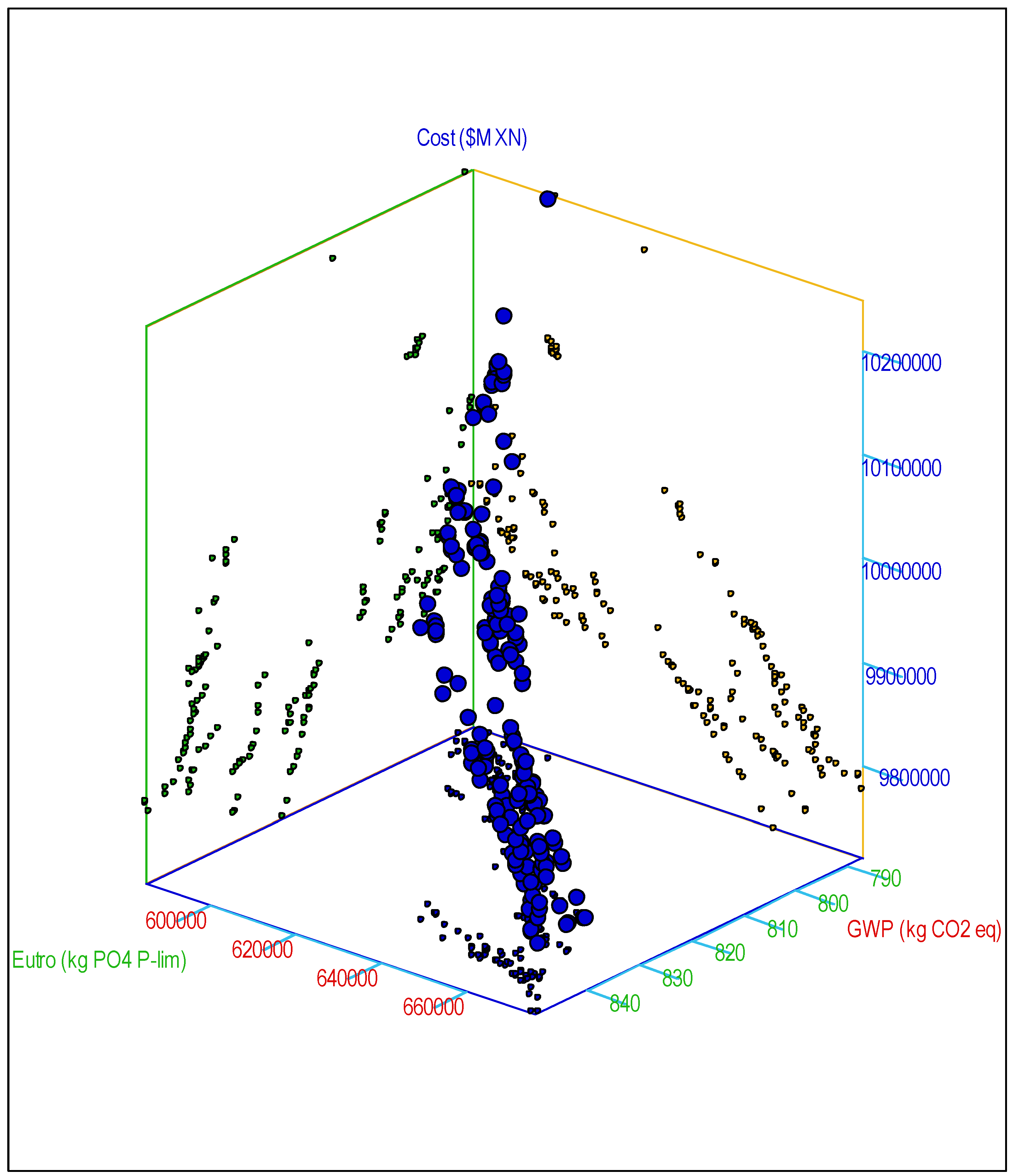
The optimization was run five times in order to validate and search a wider area of the feasible space, and this generated a set of 192 alternatives to be analyzed.
Figure 3 shows a three-dimensional scatter plot where the vertical axis is Cost (in Mexican pesos or
$MXN), the right axis is GWP (in kg CO
2 eq) and the depth axis is Eutrophication (in kg PO
4 P-lim).
Figure 3 exhibits the set of the different series of Pareto front runs. As this is a set of many Pareto fronts that were not evaluated concurrently, there are dominated points within the data set, which must be eliminated prior to applying the final selection.
Given that the resulting set of five Pareto fronts does not show a clear optimal decision alternative or region, the use of a decision-making tool becomes even more necessary. This final selection process is carried out through the use of a modified TOPSIS method proposed by Ren et al. [
45] that consists of ranking the alternatives through a comparison with the values of the “ideal” curve. Before applying the TOPSIS method, a selection is made in order to keep only non-dominated alternatives from the five Pareto fronts. This series of steps is described below:
By applying steps 1 and 2 of the abovementioned procedure, leading to the Pareto of the Paretos (i.e. Pareto {U}), a lower number of 46 non-dominated alternative solutions is obtained. From them, the TOPSIS method [
45] is applied in order to find the best ranked values.
Figure 4 shows the resulting values with the location of special TOPSIS values called 1, 13 and 45, that correspond to the overall top-ranked one, the best TOPSIS value in relation to GWP and the best TOPSIS value in relation to Eutrophication, respectively.
Figure 4 shows that the top-ranked TOPSIS value is in the higher cost range. This solution is yet selected due to the trade-off against the environmental criteria. The improvement of cost is low, relative to the gains in environmental performance.
Table 7 presents the values for each criterion for some significant TOPSIS ranked alternative: number 1 (TOPSIS 1), the 13th (TOPSIS 13) and 45th (TOPSIS 45) values. TOPSIS 1 has the best compromise since it provides the best value for GWP and only differs from the best value for Eutrophication criteria by 0.33% (TOPSIS 13). Its cost is slightly higher of 2.35% of the best cost criterion performing alternative (TOPSIS 45). The three points can also be visualized in
Figure 4 where TOPSIS 13 and 45 are at the extremes, whereas TOPSIS 1 is located at the upper part of the scatter plot.
Table 8 presents a comparison between the TOPSIS 1 solution and the TOPSIS 1 of a sample taken from the first Pareto front run at the 10
th generation. The 10
th generation was selected because it was the first generation in which all the individuals (solutions) are in the feasible space.
The differences that can be observed are significant for all criteria, which justifies the application of the optimization procedure. A comparison between the average values of the sample is used in order to visualize the improvement that can be achieved through Partnership for Sustainability method, exhibiting a significant performance between 14% to 35% for the different criterion.
Supplier contracting is then the final stage in the selection process. For the case study, the optimization results then allow to select the suppliers, the type of technological package to use, and the area of land to be guaranteed in the final contract.
Table 9 displays the final set of values for the decision variables for TOPSIS 1 alternative. It can be first observed that it implies all suppliers, since the optimization search leads to select different types of technologies of low yield but with a better overall performance. The second interesting point is that the mix of technologies used does not include technology package 3, which is the most commonly used technological package in the region. It must be also highlighted that there was only one field of a small area with a technology package type 1. This is most probably due to the fact that technology package 2 yields more products for a similar environmental impact performance.
The application of the methodology results in a set of alternatives given by rank. Although other external factors such as agricultural, economic and environmental policies have to be considered in the final judgment, the decision aid provides the insight needed for an objective and efficient supplier selection tool.

 ,
, 


