Alternative Algorithm for Automatically Driving Best-Fit Building Energy Baseline Models Using a Data—Driven Grid Search

Abstract

Change-point regression models are often used to develop building energy baselines that can be used to predict energy use and determine energy savings during a given performance period. However, the reliability of building energy baselines can depend on how well the change-point model fits the data measured during the baseline period. This research proposes the use of segmented linear regression models with one or two change points for automatically driving best-fit building energy baseline models, along with an algorithm using a data-driven grid search to find the optimal change point(s) within a given data boundary for the proposed models. The algorithm was programmed and tested with actual measured data (e.g., daily gas and electricity use) for case-study buildings. Graphical and statistical analysis was also performed to validate its reliability within acceptable deviations of an overall coefficient of variation of the root mean squared error (i.e., CV(RMSE)) of 1%, as compared to the results derived from the ASHRAE Inverse Model Toolkit (IMT) that was developed as a public domain program to manually derive the change-point model with user specified parameters. Consequently, it is expected that the algorithm can be applied for automatically deriving best-fit building energy baseline models with optimal change point(s) from measured data.

1. Introduction

Building energy baselines are required to predict energy use and determine energy savings in the measurement and verification (M&V) of building energy conservation and retrofit projects and sometimes used to identify operational problems. According to the International Performance Measurement and Verification Protocol (IPMVP) and ASHRAE Guideline 14, the whole-building M&V approach (i.e., M&V Option C) can be used as a cost-effective M&V option when energy savings are expected to be significant as compared to whole-building energy baselines [1,2,3].

Regression models with change points have long been studied in many fields to detect change-points and develop best-fit models as a function of outdoor temperature for the whole-building M&V applications. Variable-base degree-day (VBDD) model [4] was initially used in the 1980s based on heating or cooling degree-days to determine a balance-point (i.e., change-point) temperature that could give the best-fit to monthly data for single zone residential buildings. However, the VBDD model could be inappropriate for multi-zone commercial buildings with various energy use patterns.

Advanced mathematical and regression models have also been published and evaluated that offer between 3% and 7% error when developing whole-building energy baselines; these include the day-time-temperature, mean-week, change-point, and LBNL models, as well as other proprietary representations [5,6,7]. Bayesian models have sometimes been used as a probabilistic approach to realistically quantify the uncertainty of energy savings and regression models with outliers for M&V applications [8]. Among the published models, the change-point models with certain parameters defined in ASHRAE Guideline 14 have widely been applied to develop whole-building energy baselines for various M&V projects [9,10,11,12]. For instance, a two-parameter model (i.e., linear regression model) has normally been applied for heating or cooling energy baselines as a linear function of outdoor temperature, whereas three-parameter and four-parameter models have frequently been applied to capture a certain change-point affected by system controls for multi-zone residential and commercial buildings equipped with heating, ventilation, and air-conditioning (HVAC) systems. Five-parameter model can be extended to apply for both heating and cooling energy baselines with two change-points at the same time.

The ASHRAE Inverse Model Toolkit (IMT) [13,14] was developed as a public domain program to develop such whole-building energy baseline models in compliance with the ASHRAE Guideline-14P, but its use is to manually derive the change-point baseline models with user specified parameters. The IMT used a two-stage, step-sized (i.e., ten increments) grid search method based on an equal temperature interval to drive best-fit change-point(s) regression models and then estimated model coefficients using least-squares regression analysis; such a method has proven to be robust to find a certain change-point within a given data (e.g., outdoor temperature) boundary, but the location of change-point(s) could depend on the grid interval (i.e., step size) predefined in the IMT.

Segmented linear regression [15,16] has been considered as one of the most accurate ways to estimate the exact position of change point(s) and model parameters when two regression lines are continuous. However, it could sometimes lie outside of a given data range when a number of abnormal measured data are biased on either side of segmented regression line. To overcome this issue, this research proposes the use of segmented linear regression models with continuity constraints for driving best-fit building energy baselines, and also presents an enhanced algorithm using a data-driven grid search to estimate the optimal change point(s) within a given data boundary for the proposed models.

Validation of the best-fit change-point regression model is crucial for developing a whole-building energy baseline at an acceptable level of accuracy. According to ASHRAE Guideline 14 [2], the accuracy of a change-point regression model can normally be evaluated using the coefficient of determination (R²) and the coefficient of variation of the root mean squared error (CVRMSE). Additional statistical metrics such as normalized root mean square error (nRMSE), median absolute relative total error (med(absRTE)), and relative bias (relBias) have sometimes been used to characterize the predictive accuracy of building energy baseline models during certain training (i.e., baseline) periods [5,6,7]. For the present study, the statistical metrics (e.g., CV(RMSE) and R²) were adapted to automatically validate the best-fit baseline model derived from actual measured data during a baseline period.

Paulus et al. proposed an algorithm to automate the process of selecting an appropriate change-point model through a series of three tests, addressing model shape, significance of the model coefficients, and minimum number of data points [17]. The algorithm appeared to be helpful for selecting a physically reasonable whole-building baseline model, but their tests were limited to synthetic monthly energy data. The present study proposes a simplified algorithm to automatically select the best-fit baseline model within a given data boundary and verifies its reliability with actual measured data (e.g., daily gas and electricity use) through statistical and graphical comparisons.

This research proposes the use of segmented linear regression models with one or two change points for driving the best-fit building energy baseline model from measured data, along with an algorithm using a data-driven grid search to find the optimal change point(s) within a given data boundary for the proposed models. The algorithm was programmed to automatically drive the best-fit building energy baseline model and tested with actual measured data (e.g., daily gas and electricity use) for case-study buildings. Graphical and statistical comparisons (e.g., R² and CV(RMSE)) were also performed to validate its reliability during a heating and cooling baseline period.

The rest of this paper is structured as follows: The materials and methods for deriving segmented linear regression models with optimal change-points are described in Section 2. The statistical and graphical results of the best-fit building energy baseline models automatically derived from actual measured data for the case-study buildings are demonstrated in Section 3. The discussion regarding the proposed models with algorithms, statistical and graphical results, and patent applications are presented in Section 4. Finally, conclusions are drawn in Section 5.

2. Materials and Methods

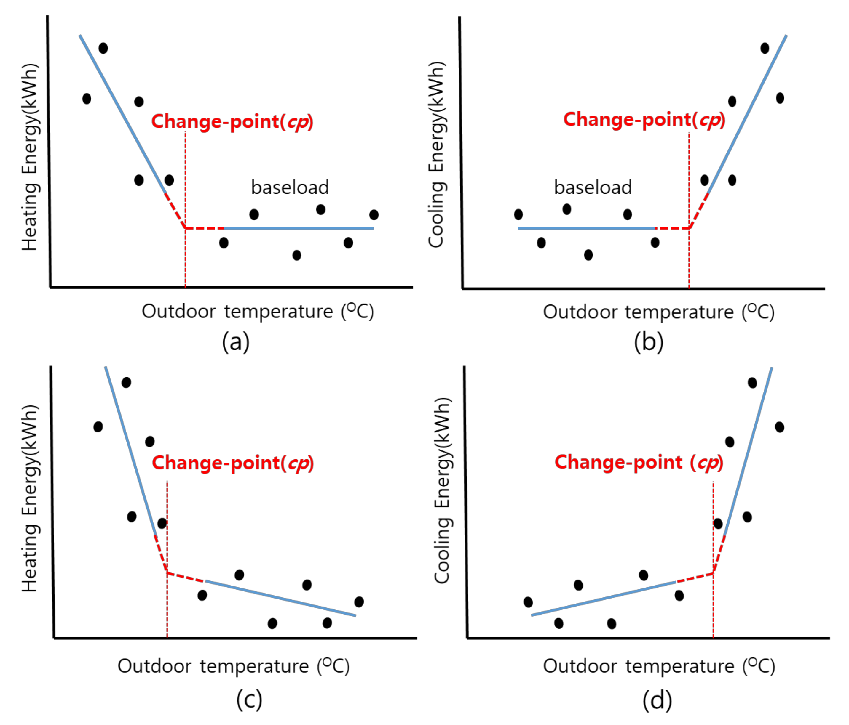
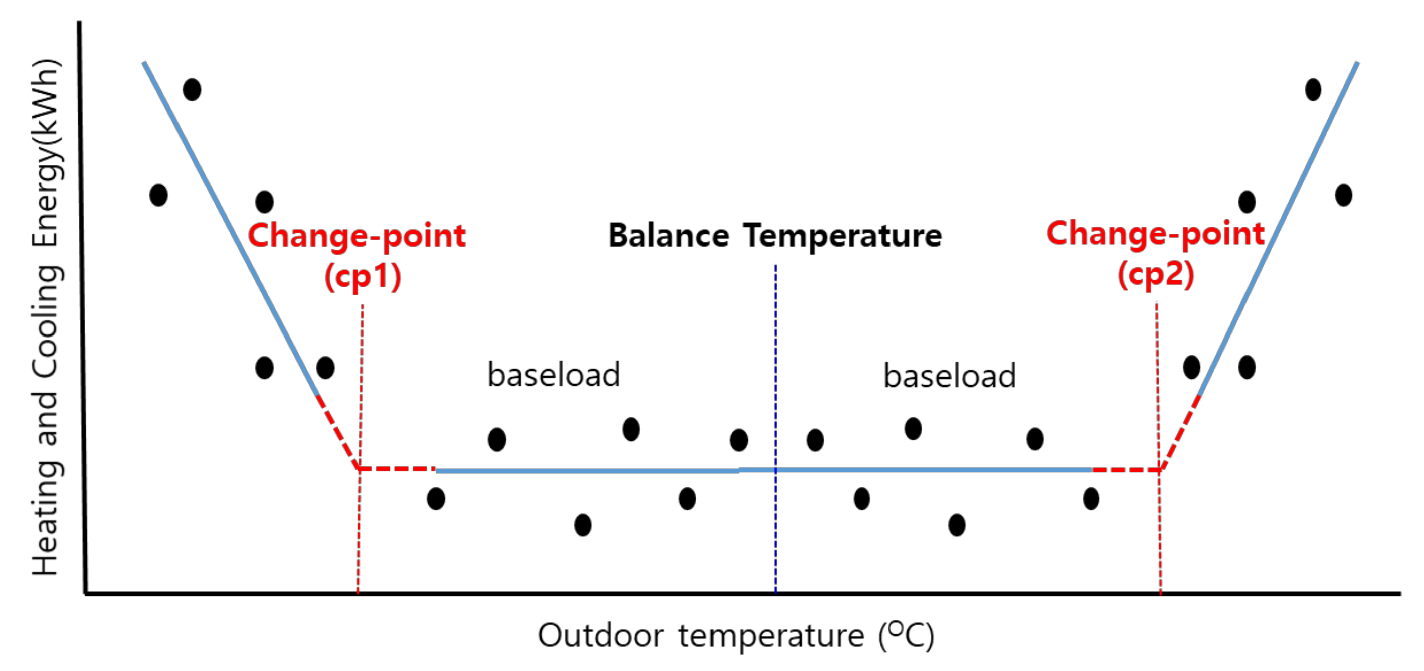
2.1. Segmented Linear Regression Models with One or Two Change Points

Building energy consumption can typically be represented as a piecewise linear function of outdoor temperature with a certain change point, which is generally affected by operational conditions (e.g., heating or cooling set-point temperature) for heating, ventilation, and air conditioning (HVAC) systems. Relatedly, this study proposes segmented linear regression models with one or two change-point temperatures, as shown in Figure 1 and Figure 2. The segmented linear regression models proposed in this study appear to be similar to the parameters-based change-point linear regression models described in ASHRAE Guideline 14 [2]. However, the method of exploring the change point(s) is different from the step-sized grid search process used in the IMT. This study adapts a data-driven grid search method to explore the optimal change point(s) for the following segmented linear regression models.

Linear regression models with no change points are generally defined as in Equations (1) and (2); model coefficients can be determined using a least-squares regression algorithm. Equation (1) represents a constant energy model (or mean model), while Equation (2) stands only for a heating or cooling energy model as a function of an independent variable (e.g., outdoor temperature). These two models are the same as the one- or two-parameter models used in the IMT.

$$E_i= {\beta }_0+e_i$$

(1)

$$E_i= {\beta }_0+{\beta }_1{T}_i+e_i,$$

(2)

where $E_i$ is the energy consumption, ${\beta }_0$ is the E-intercept, ${\beta }_1$ is the left or right slope, $T_i$ is the outdoor temperature, and $e_i$ is the error.

The segmented linear regression models with one or two change points are proposed in this study using Equations (3)–(6). Equations (3) and (4) represent a heating or cooling change-point model with a slope, while Equation (5) demonstrates a heating or cooling change-point model with two slopes. As shown in Figure 1a–d, these models with a change point can be used only for heating or cooling energy baselines, similar to the three- and four-parameter models in the IMT. Equation (6) represents both heating and cooling change-point models with two slopes, as shown in Figure 2. Here, the segmented linear regression models are connected at the change point (i.e., cp) under the following conditions. No change-point model in Equation (1) or Equation (2) should be automatically selected as an alternative model in the program developed for this study If the denominators (e.g., ${\beta }_1, {\beta }_3, {\beta }_1-{\beta }_3, and {\beta }_4)$ of change-point(s) in the Equations (3)–(6) happen to be equal to zero, which seldom occurred in practice.

$$E_i=\left\{\begin{array}{c}{\beta }_0+{\beta }_1{T}_i+e_i, T_i\le cp\\ {\beta }_2+e_i, cp<T_i\end{array}\right.,$$

(3)

where ${\beta }_0+{\beta }_{1}cp={\beta }_2$, $cp=\frac{{\beta }_2-{\beta }_0}{{\beta }_1}$,

$$E_i=\left\{\begin{array}{c}{\beta }_2+e_i, T_i\le cp \\ {\beta }_0+{\beta }_3{T}_i+e_i, cp<T_i\end{array}\right.,$$

(4)

where ${\beta }_0+{\beta }_{3}cp={\beta }_2$, $cp=\frac{{\beta }_2-{\beta }_0}{{\beta }_3}$,

$$E_i=\left\{\begin{array}{c}{\beta }_0+{\beta }_1{T}_i+e_i, T_i\le cp \\ {\beta }_4+{\beta }_3{T}_i+e_i, cp<T_i\end{array}\right.,$$

(5)

where ${\beta }_0+{\beta }_{1}cp={\beta }_4+{\beta }_{3}cp$, $cp=\frac{{\beta }_4-{\beta }_0}{{\beta }_1-{\beta }_3}$,

$$E_i=\left\{\begin{array}{c}{\beta }_0+{\beta }_1{T}_i+e_i, T_i\le c{p}_1\\ {\beta }_2+e_i, c{p}_1<T_i\le c{p}_2\\ {\beta }_4+{\beta }_3{T}_i+e_i, c{p}_2<T_i\end{array}\right.,$$

(6)

where $c{p}_1=\frac{{\beta }_2-{\beta }_0}{{\beta }_1}$ and $c{p}_2=\frac{{\beta }_2-{\beta }_3}{{\beta }_4}$,

where, E $\mathrm{is}$ the energy consumption; ${\beta }_{0 },$ ${\beta }_2$, or ${\beta }_{4 }$ is the E-intercept; ${\beta }_1$ is the left slope; ${\beta }_3$ is the right slope; $T_i$ is the outdoor temperature; $e_i$ is the error; and $cp$ is the change-point temperature.

2.2. Algorithm for Exploring the Optimal Change Point(s)

This study presents an algorithm using a data-driven grid search method to find the exact change point(s) for the segmented linear regression models proposed herein. The procedure for exploring one (i.e., A-1CP) or two (i.e., A-2CP) change points for the segmented regression models is shown in Figure 3 and described below.

(1)

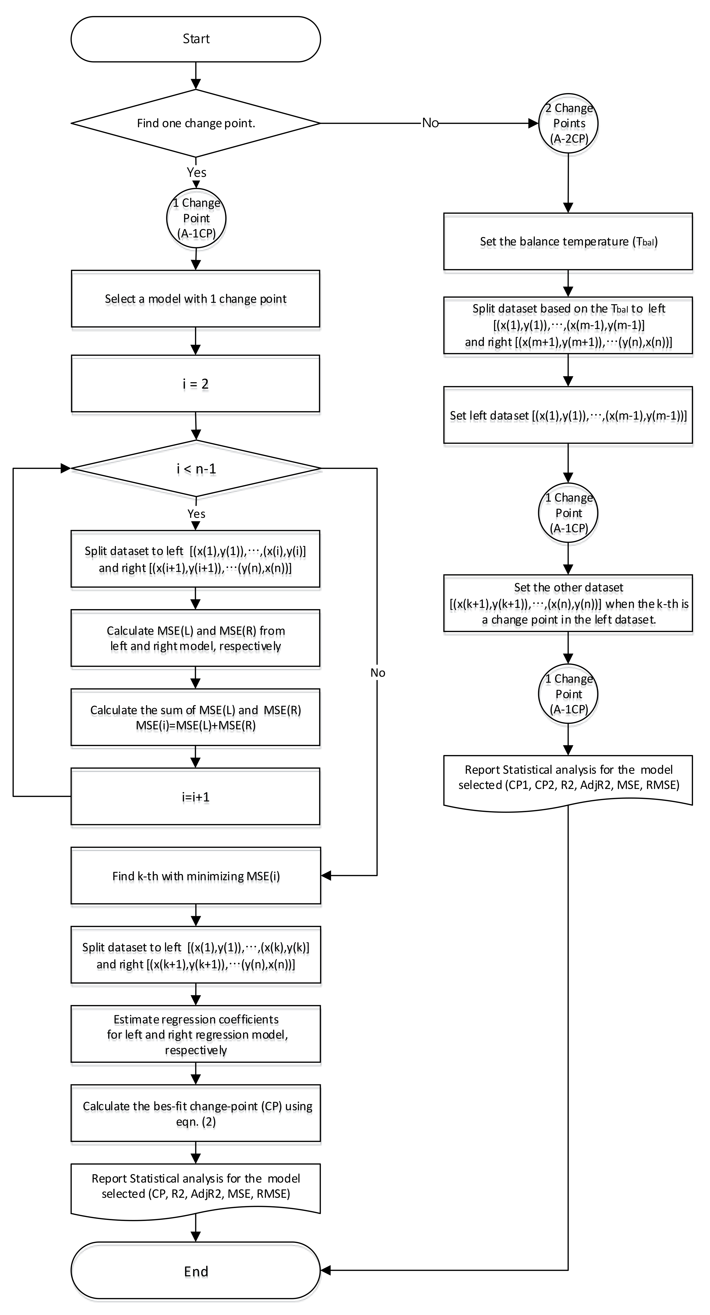
A-1CP algorithm to detect one change point

To detect one change point from the segmented regression models illustrated in Figure 1, the dataset ${\left\{\left(E_i,T_i\right)\right\}}_{i=1}^n$ was first split into left and right datasets, based on the initial datapoint (i.e., i = 2), and then the sum of the mean square error (MSE(i)) was calculated from the MSE(L) of the left model and MSE(R) of the right model. The calculation process for MSE(i) was repeated sequentially from the initial datapoint (i.e., i = 2) to the second to last datapoint (i.e., i = n − 2), based on the data-driven grid search method. Next, to estimate the exact change point (CP), the dataset was split into left and right datasets, again based on a certain datapoint (i.e., k) with a minimum MSE(i), and the intersection of the left and right models was then calculated. A statistical analysis (e.g., overall R², RMSE, CV(RMSE)) was finally performed to estimate the overall accuracy of the selected model.

< Step 1 >

Set a dataset including only one change: $\left(E_1,T_1\right)$, …, $\left(E_n,T_n\right)$.

< Step 2 >

Set the dataset as one model in Equation (1) or Equation (2).

< Step 3 >

Repeat $\mathrm{i}=2:\mathrm{n}-2 \{$.

• (3-1) Calculate MSE(L) from $\left(E_1,T_1\right)$, …, $\left(E_i,T_i\right)$ using the left model.
• (3-2) Calculate MSE(R) from $\left(E_{i+1},T_{i+1}\right)$, …, $\left(E_n,T_n\right)$ using the right model.
• (3-3) Calculate MSE(i) = MSE(L) + MSE(R)}.

< Step 4 >

Find the position $k$ ($2\le k\le n-2$) such that it minimizes the MSEs.

< Step 5 >

Split the dataset into $\left(E_1,T_1\right)$, …, $\left(E_k,T_k\right)$ and $\left(E_{k+1},T_{k+1}\right)$, …, $\left(E_n,T_n\right)$.

< Step 6 >

Model $\left(E_1,T_1\right)$, …, $\left(E_k,T_k\right)$ as the left model and the other dataset as the right model.

< Step 7 >

Estimate the change point (i.e., CP) by calculating the intersection of the left and right models.

< Step 8 >

Analyze the model with one change point given and report the overall statistical properties (e.g., change point, left or right slope, overall R², RMSE, CV(RMSE)).

(2)

A-2CP algorithm to detect two change points

The segmented regression model with two change points, as illustrated in Figure 2, can also be developed based on the procedure outlined in Figure 3. To detect two change points in the segmented regression model, the dataset was first split into left and right datasets based on the balance temperature (e.g., average outdoor temperature of the given dataset), and then the calculation process for MSE(i) was repeated until the change point (i.e., CP₁) was detected from left dataset using the data-driven grid search method (in a way similar to the algorithm for detecting one change point). Next, the right dataset was redefined from CP₁ to the last datapoint. Then, the data-based grid search was repeated until the change point (i.e., CP₂) was detected. A statistical analysis (e.g., overall R², RMSE, CV(RMSE)) was finally performed to estimate the overall accuracy of the selected model as well.

< Step 1 >

Set a balance temperature to separate each dataset with only one change point:

• $\left(E_1,T_1\right)$, …, $\left(E_{m-1},T_{m-1}\right)$, $T_1,\dots ,T_{m-1}\le T_{bal}.$

< Step 2 >

Conduct A-1 CP with this dataset and find one change point, $k1 \left(i.e., C{P}_1\right).$

< Step 3 >

Set the other dataset with one change point: $\left(E_{k1+1},T_{k1+1}\right)$, …, $\left(E_n,T_n\right)$.

< Step 4 >

Conduct A-1 CP with the other dataset and find the other change point, $k2 \left(i.e., C{P}_2\right)$.

< Step 5 >

Set three datasets based on two change points:

• $[\left(E_1,T_1\right)$, …, $\left(E_{k1},T_{k1}\right)$], [$\left(E_{k1+1},T_{k1+1}\right)$, …, $\left(E_{k2},T_{k2n}\right)]$ and $[\left(E_{k2+1},T_{k2+1}\right)$, …, $\left(E_n,T_n\right)$

< Step 6 >

Determine the final two change points (i.e., CP₁ and CP₂).

< Step 7 >

Perform regression analyses for the model with two change points and report the overall statistical results (e.g., left and right change points, left and right slope(s), overall R2, RMSE, CV(RMSE)).

2.3. Validation Metrics for the Best-Fit Change-Point Regression Model

Validation of the best-fit change-point regression model is crucial in developing reliable building energy baselines within acceptable levels of accuracy. According to ASHRAE Guideline 14 [2], the accuracy of a change-point regression model can be evaluated using statistical metrics such as the coefficient of determination (R²) and coefficient of variation of the root mean squared error (CVRMSE). The R² value generally represents how well a regression model describes the variability of the measured data, while the root mean square error (RMSE) is a measure of the differences between the measured and predicted model data. The CV(RMSE) can be calculated by dividing the RMSE by the mean value of the measured data, as shown in the Equation A1 of Appendix A. Additional statistical metrics such as normalized root mean square error (nRMSE), median absolute relative total error (med(absRTE)), and relative bias (relBias) have sometimes been used to characterize the predictive accuracy of building energy baseline models during different training (i.e., baseline) periods [5,6,7]. In the present study, a simplified algorithm was programmed to automatically select the best-fit baseline model with the lowest CV(RMSE) among the proposed segmented linear regression models; this was then tested with actual measured data (e.g., daily gas and electricity use) to validate its reliability with the statistical validation metrics (e.g., CV(RMSE) and R²). Graphical comparisons (e.g., model shape) were also performed to identify the best-fit baseline model during a heating and cooling baseline period.

3. Results

The algorithm was programmed to automatically drive the best-fit building energy baseline model within a given data boundary and tested with actual measured data (e.g., daily gas or electricity use) for absorption chillers/heaters and related equipment (e.g., pumps and cooling towers) in case-study buildings, which are served by a central heating and cooling plant. Graphical identification and statistical analysis (e.g., R² and CV(RMSE)) were also performed to validate its reliability, as compared to the results derived from the ASHRAE IMT during a heating and cooling period.

3.1. Measured Datasets

The case-study buildings located in Suwon city, Korea are composed of three office buildings served by a central heating and cooling plant, which includes three gas-fired absorption chillers/heaters, three circulation pumps, three cooling towers, and electric panels with motor control centers (MCCs). For this study, a central monitoring system were installed to measure hourly gas consumption from the three gas-fired absorption chillers/heaters, as well as the electricity use from the motor control center (MCC) panels connected to the central circulation pumps and cooling towers for the absorption chillers/heaters.

Table 1. Description of heating and cooling plants metered.

Types	Descriptions	Meters Installed	Measurement Periods	Remarks
Absorption chiller-heaters	240RT (COP 1.2) 400RT (COP 1.2) 450RT (COP 0.7)	Gas-meters (3EA)	1 February–11 March	Heating
			1 June–13 September	Cooling
			1 November–16 December	Heating
Pumps	Circulation Pumps (3EA)	Electric power meter (MCC Panel)	1 February–16 December	Heating
Cooling Towers	Open Towers (3EA)		1 June–13 September	Cooling

summarizes the heating and cooling plant with equipment metered. For this study, measured hourly data were converted into daily datasets (except for weekends and holidays) for 11 months, from 1 February to 16 December 2016, and then were used to drive the best-fit change-point baseline models during the heating and cooling baseline period.

3.2. Comparisons of the Best-Fit Baseline Models During the Heating and Cooling Period

Table 2. Statistical results of the proposed gas and electricity baseline models during the heating and cooling periods.

Items (Units)	Model Type	Number of Data	R2	CVRMSE (%)	Change Point			Remarks
					Xcp1	Xcp2	Ycp
Absorption chiller/heater (Gas, m3)	1CP Heating	72	0.09	64.92	1.37	−	621.68	Not acceptable
	1CP Cooling	72	0.56	45.13	−	27.22	416.39	Not acceptable
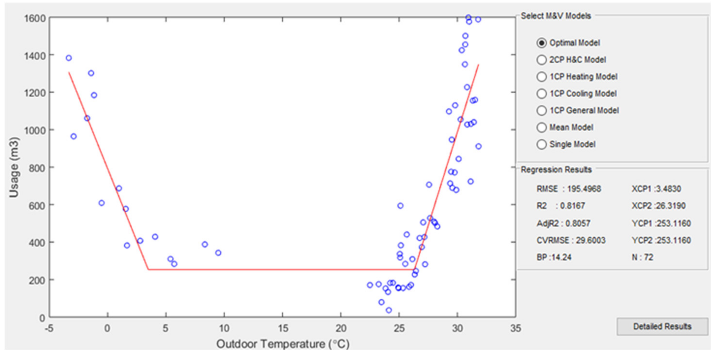
	2CP H&C	72	0.82	29.60	3.48	26.32	253.12	Best-fit
	IMT 5P	72	0.82	29.32	3.17	26.61	268.35	Best-fit
	Deviation (%)	0	0.00 (0.2%)	−0.28 (0.9%)	−0.31 (8.9%)	0.29 (1.1%)	15.24 6.0(%)	2CP H&C –IMP 5P
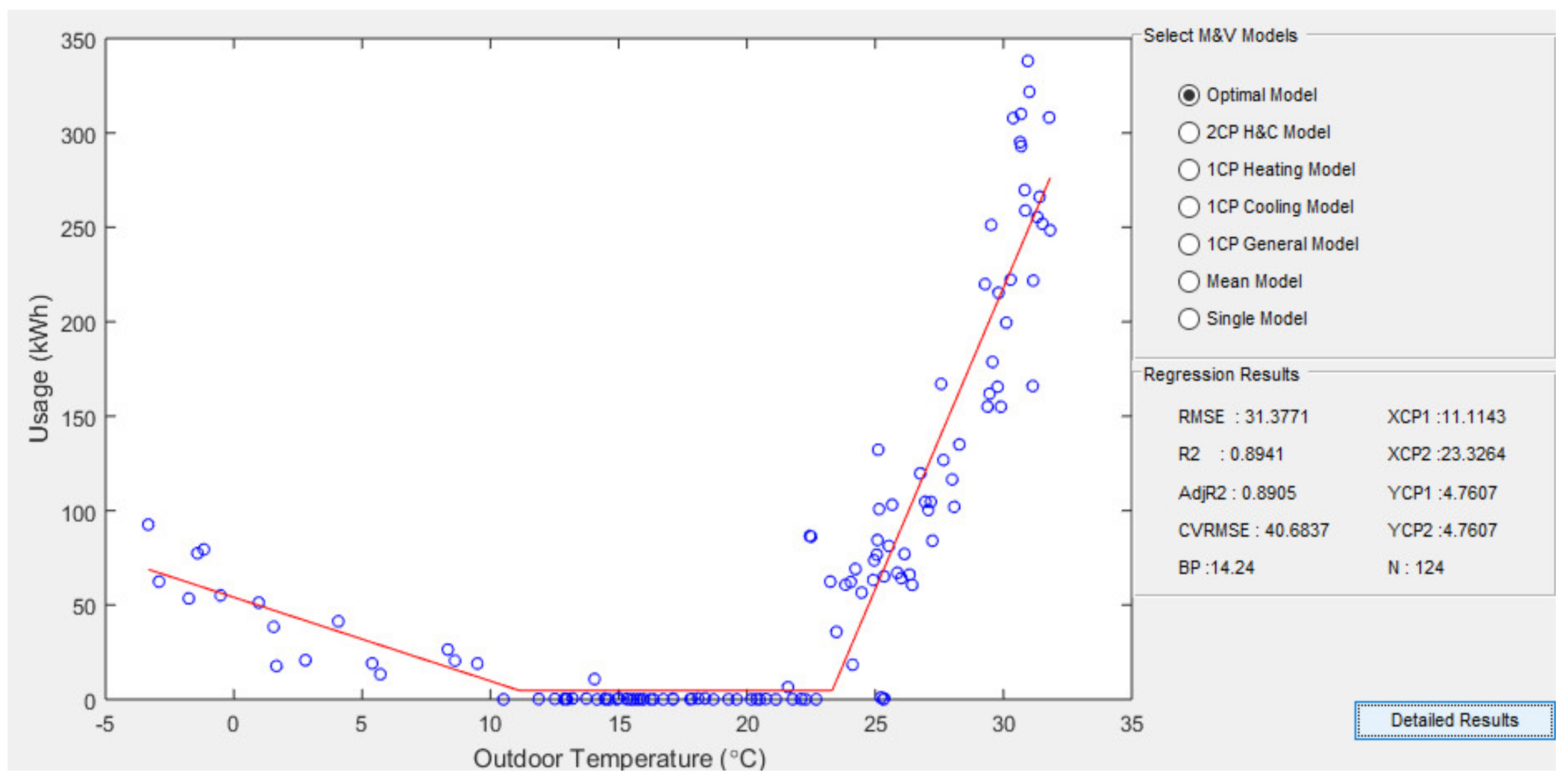
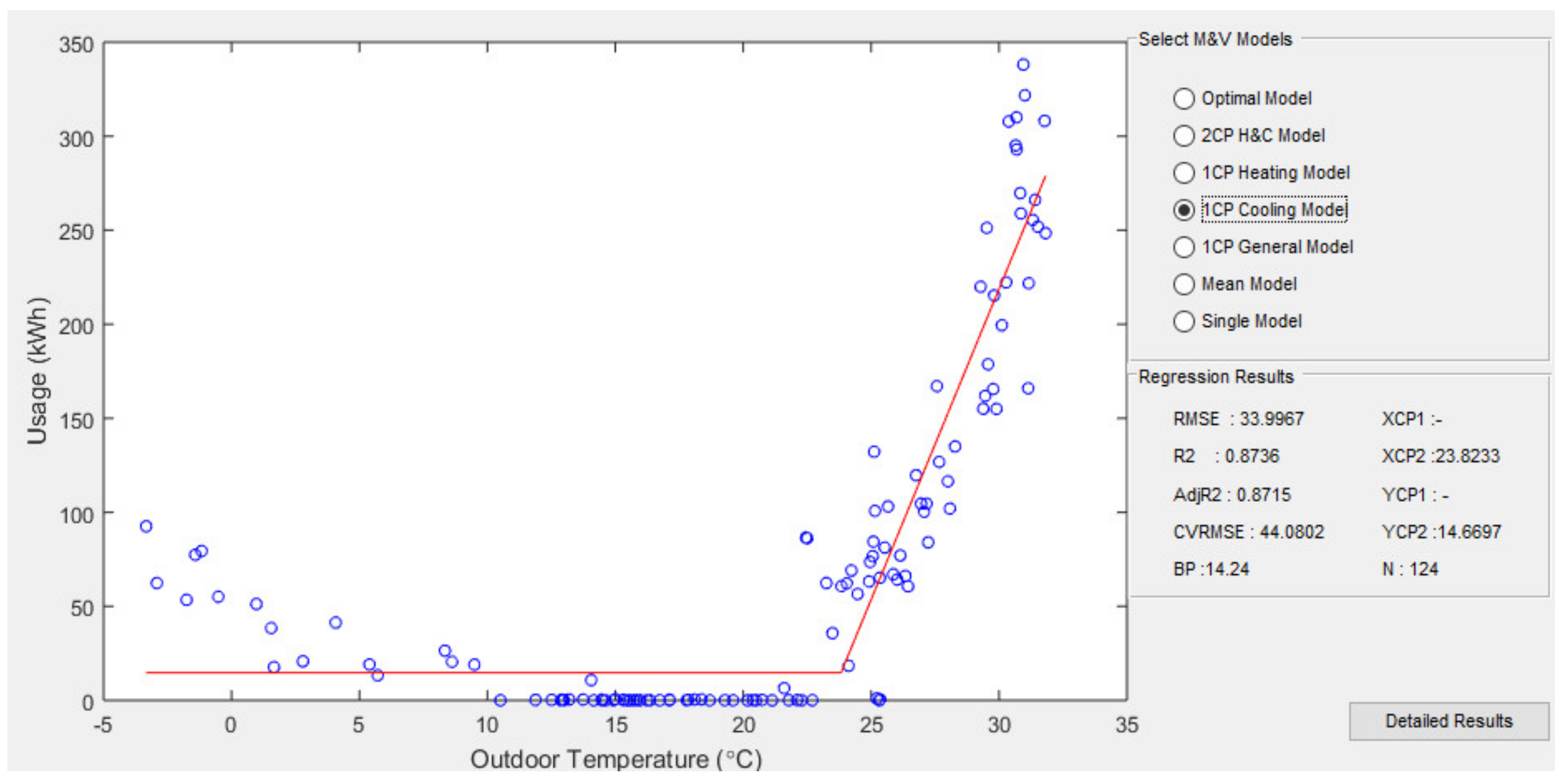
Pumps and cooling towers (Electricity, kWh)	1CP Cooling	124	0.87	44.08	−	23.82	14.67	Not acceptable
	2CP H&C	124	0.89	40.68	11.11	23.33	4.76	Best-fit
	IMT 5P	124	0.89	40.55	4.47	23.33	10.32	Best-fit
	Deviation (%)	0	0.00 (0.1%)	−0.14 (0.3%)	−6.64 (59.8%)	0.68 (2.9%)	5.55 (116.7%)	2CP H&C –IMP 5P

summarizes the statistical results of the segmented regression models derived from the measured daily gas and electricity use by absorption chillers/heaters and related equipment (e.g., pumps and cooling towers) for the case-study building during the heating and cooling period from 1 February to 16 December 2016.

For the measured daily gas consumption, a 2CP heating and cooling (H&C) model was automatically selected as the best-fit baseline model with the lowest CV(RMSE) of 29.60%, as compared to the other proposed models, such as the ICP heating model with a CV(RMSE) of 64.92% and 1CP cooling model with a CV(RMSE) of 45.13%. The 2CP H&C model was also graphically identified as the best-fit baseline model with two change points, as shown in Figure 4. The 2CP H&C model was in good agreement with the statistical results of the IMT 5P model, along with an R² deviation of 0.0017(0.2%) and CV(RMSE) of 0.2793(0.9%). The Xcp1, Xcp2, and Ycp change points were shifted slightly from those of the IMT 5P model, along with acceptable deviations of 0.31 °C (5.9%), 0.29 °C (1.1%), and 15.2 m³ (6%), respectively.

For electricity use by pumps and cooling towers, the 2CP H&C model was also automatically selected as the best-fit baseline model because it had the lowest CV(RMSE) of 40.68% among the proposed models, as shown in Table 1. The 2CP H&C model was also graphically identified as the best-fit baseline model, as shown in Figure 5. In addition, the 2CP H&C model was in good agreement with the IMT 5P model, along with an R² deviation of 0.0011(0.1%) and CV(RMSE) of 0.1377(0.3%). However, the Xcp2 and Ycp change points were significantly shifted from the IMT 5P model, along with deviations of 6.64 °C (59.8%) and 5.6 kWh (116.7%), respectively, while the deviation of the Xcp1 change point was only 0.68 °C (2.9%). The ICP cooling model also seemed to be statistically acceptable, with an R² of 0.876 and CV(RMSE) of 44.08% (as compared to the 2CP H&C model shown in Table 1). However, the graphical result in Figure 6 shows that the gas energy use below the Xcp2 change point (23.32 °C) appeared to be mismatched with the 1CP cooling model.

4. Discussion

The segmented linear regression models proposed in this study appear to be similar to the parameters-based change-point linear regression models described in ASHRAE Guideline 14 [2]. However, the method of exploring the change point(s) is different from the step-sized grid search process used in the IMT. This study adapts a data-driven grid search method to explore the optimal change point(s) for the segmented linear regression models.

The algorithm was programmed to drive the best-fit change point model within a given data boundary and tested with actual measured data (e.g., daily gas and electricity use) for absorption chillers/heaters and related equipment (e.g., pumps and cooling towers) in case-study buildings. The results show that the best-fit baseline models with optimal change point(s) were within acceptable deviations of an overall CV(RMSE) of 1%, as compared to the results derived from the ASHRAE Inverse Model Toolkit (IMT) used as a public domain program. However, the deviations of change points (e.g., outdoor temperature) for each model varied from 0.29 °C to 6.6 °C, due to the algorithm for exploring the optimal change point(s) based on the data-driven grid search proposed in this study.

The algorithm proposed in this study was used to apply for the patent referenced in Section 6—A system for measuring and evaluating building energy performance and method, which includes several related modules integrated with an automatic M&V system.

5. Conclusions

This research proposes segmented linear regression models with one or two change points for automatically driving best-fit building energy baselines, along with an algorithm to explore the optimal change point(s) based on a data-driven grid search method. The best-fit baseline models derived from the measured data were validated within acceptable deviations of an overall CV(RMSE) of 1% and R² of 0.001, as compared to the results from the ASHRAE IMT that was developed as a public-domain program, but its use was to manually derive the change-point baseline model with user specified parameters. Consequently, it is expected that the algorithm can be used as an alternative for automatically deriving best-fit building energy baseline models with optimal change point(s) from measured data. However, the accuracy of a building energy baseline model could sometimes be affected by not only outdoor temperature but also other variables (e.g., humidity) and abnormal energy data called outliers, which need to be further considered for future works.

6. Patents

PCT/KR2016/013835 “System for measuring and evaluating building energy performance and method for driving same” (http://www.ic.gc.ca/opic-cipo/cpd/eng/patent/3005184/summary.html? query=(Pending+Applications+%3CIN%3E+STATUS)&start=1&num=50&type=advanced_search&pedisable=true).

References

- EVO. International Performance Measurement and Verification Protocol: Concept and Options for Determining Energy and Water Savings; Efficiency Valuation Organization (EVO): Washington, DC, USA, 2012. [Google Scholar]
- ASHRAE. ASHRAE Guideline 14-2014 for Measurement of Energy, Demand, and Water Savings; American Society of Heating, Refrigeration, and Air Conditioning Engineers: Atlanta, GA, USA, 2014. [Google Scholar]
- FEMP. M&V Guidelines: Measurement and Verification for Performance-Based Contracts Version 4.0; Federal Energy Management Program, Energy Efficiency& Renewable Energy: Washington, DC, USA, 2015. [Google Scholar]
- Fels, M.F. PRISM: An introduction. Energy Build. 1986, 9, 5–18. [Google Scholar] [CrossRef]
- Granderson, J.; Price, P.N. Development and application of a statistical methodology to evaluate the predictive accuracy of building energy baseline models. Energy 2014, 66, 981–990. [Google Scholar] [CrossRef]
- Granderson, J.; Price, P.N.; Jump, D.; Addy, N.; Sohn, M.D. Automated measurement and verification: Performance of public domain whole-building electric baseline models. Appl. Energy 2015, 144, 106–113. [Google Scholar] [CrossRef]
- Granderson, J.; Touzani, S.; Custodi, C.; Sohn, M.D.; Jump, D.; Fernandes, S. Accuracy of automated measurement and verification (M&V) technologies for energy savings in commercial buildings. Appl. Energy 2016, 173, 296–308. [Google Scholar]
- Carstens, H.; Xia, X.; Yadavalli, S. Bayesian energy measurement and verification analysis. Energies 2018, 11, 380. [Google Scholar] [CrossRef]
- Haberl, J.S.; Thasmilseran, S.; Reddy, T.A.; Claridge, D.E.; O’Neal, D.; Turner, W.D. Baseline calculations for measurement and verification of energy and demand savings in a revolving loan program in Texas. ASHRAE Trans. 1998, 104, 841–858. [Google Scholar]
- Song, S.; Haberl, J.S. Analysis of the impact of using synthetic data correlated with measured data on the calibrated as-built simulation of a commercial building. Energy Build. 2013, 67, 97–107. [Google Scholar] [CrossRef]
- Perez, K.X.; Cetin, K.; Baldea, M.; Edgar, T.F. Development and analysis of residential change-point models from smart meter data. Energy Build. 2017, 139, 351–359. [Google Scholar] [CrossRef]
- Golden, A.; Woodbury, K.; Carpenter, J.; O’Neill, Z. Change point and degree day baseline regression models in industrial facilities. Energy Build. 2017, 144, 30–41. [Google Scholar] [CrossRef]
- Kissock, J.K.; Haberl, J.S.; Claridge, D.E. Development of a Toolkit for Calculating Linear, Change-Point Linear and Multiple-Linear Inverse Building Energy Analysis Model; Final Report; ASHRAE: Atlanta, GA, USA, 2002. [Google Scholar]
- Kissock, J.K.; Haberl, J.S.; Claridge, D.E. Inverse Modeling Toolkit: Numerical Algorithms. ASHRAE Trans. 2003, 109, 425. [Google Scholar]
- Lerman, P.M. Fitting segmented regression models by grid search. Appl. Stat. 1980, 29, 77–84. [Google Scholar] [CrossRef]
- Chen, C.W.S.; Chan, J.S.K.; Gerlach, R.; Hsieh, W.Y.L. A comparison of estimators for regression models with change points. Stat. Comput. 2011, 21, 395–414. [Google Scholar] [CrossRef]
- Paulus, M.T.; Claridge, D.E.; Culp, C. Algorithm for automatic the selection of a temperature dependent change point model. Energy Build. 2015, 87, 95–104. [Google Scholar] [CrossRef]