Application of Fractal and Gray-Level Co-Occurrence Matrix Indices to Assess the Forest Dynamics in the Curvature Carpathians—Romania

Abstract

The mountain ecosystems face significant damage from deforestation and environmental forest changes. We investigated the evolution of tree types of cover areas, deforested areas and total deforested areas from Curvature Carpathians using Gray-Level Co-occurrence Matrix and fractal analysis. The forest dynamics mapping was one of the main objectives of this study and it was carried out using multiple fractal and GLCM indices. We approached the analysis of satellite forest images by calculation of four fractal indices such as Pyramid dimension, Cube Counting Dimension, Fractal Fragmentation-Compaction Index and Tug-of-War lacunarity. We also calculated fractal dimension because it is an index of complexity comparing how the detail in a pattern changes with the scale at which it is measured. Fractal dimension is useful for estimation of irregularity or roughness of fractal and natural objects that do not conform to Euclidian geometry. While the fractal dimension quantifies how much space is occupied, the Tug-of-War lacunarity complements fractal dimension with its ability to quantify how space is occupied. Analysis was further supplemented by the Gray-Level Co-occurrence Matrix analysis because it quantifies spatial probability distributions of gray level values between pixel pairs within an image. The calculated Gray-Level Co-occurrence Matrix features included Angular Second Moment, Contrast, Correlation, Inverse Difference Moment and Entropy. Such comprehensive analysis has the advantage of combining fractal analysis that extracts quantitative information about the morphological complexity of the image with the spatial distribution of the gray pixel intensities as calculated by the co-occurrence features provided by Gray-Level Co-occurrence Matrix. Evolution of deforested areas, expansion of agricultural land and the increased demand for quality timber have affected the forests ecosystems and, the regional sustainable development of local communities.

1. Introduction

In Earth ecosystems, human activity influences the biodiversity, climate change and a natural order of ecosystems by inducing new pressure elements such as habitats restraining, increasing the species competitivity and migration because of lack of food resources—nourishment. The frequency of extreme events occurs, once they were considered “exceptional” and relegated to long turnaround times, and they led to reconsider the carrying capacity of rivers and the downsizing of the banks enough to contain the floods no longer [1,2]. The forest resources are reduced due to timber production [3] and legal or illegal practices [1] together with climate change in Europe [4,5,6]. Forest areas have increased over the centuries, but after World War II, in socialist countries from South-Eastern Europe the forest areas dramatically decreased because of a high percentage of state-owned forests in Romania (31.2%) [4].

The political changes in the post-socialist period resulted in rapid modification of regulations [7], which liberalized deforestation. Forest management and large forest harvest in Curvature Carpathians are reflected in the increase of forest cover from 1924 to 2014 from 20.1% to 70% [1]. The annual forest disturbance was lower from 2000–2013 (0–0.5%) than 1912–1922 (0.6–1.5%). Percentage of forest in Romania was 25.47% between 1900–1920 with a predominance of deciduous species (52%), coniferous species (25%) and oaks (23%) [1,8]. The Food and Agriculture Organization of the United Nations (FAO) Report from 1986 confirmed that 66% of the forests in Romania are found in the mountains (30% of the country) [9]. From the 1.529 million ha of non-state forests that represent 23% of the total forest area of Romania in 2010, the harvested volume exceeded 5.89 million m³ and the total annual turnover on the private forest properties was 107 million euros [9,10,11].

The forests are under the property of state and private property of individuals and legal entities (associations, schools or churches) [12].

World Wide Fund for Nature (WWF) supports the biodiversity protection of Romanian virgin forests on the UNESCO‘s World Heritage List [13,14]. The forests in the Carpathians represent one of the Europe‘s largest virgin forests, with high ecological value. Carpathian forest have been converted for, economic activities [15,16,17] and urban development [1,11,18]. In last decades, the forests of Romania have been studied using novel methodologies, including fractal analysis [16,19,20,21] of satellite images [11,18,22,23].

The results of these studies indicate that forests of Romanian Carpathians have suffered damage, such as diminution of forest areas and reduction of biodiversity [1,24,25,26]. These changes resulted in a continuous decrease of forest areas and increase of urban development [27], expansion of agriculture croplands [15,28,29], climate change [15] and natural hazards [30]. Environmental sensitivity is defined in terms of various indicators that represent the physical situation of the forests (including the state property and its territorial context), in relation to the protection rules system that emphasizes its value [2].

In this study, we investigated the spatio-temporal evolution of tree cover areas, yearly deforested areas and total deforested areas, as a sum of all yearly deforested areas in the Curvature Carpathian forests in Romania by analysis of Landsat archive data from Global Forest Change (GFC) by fractal and Gray-Level Co-occurrence Matrix (GLCM) algorithms.

This report highlights the importance of forest dynamics in deforested areas and tree cover areas in Curvature Carpathians. Accordingly, our goal here was to quantify the forest diminution across the study area, from 2000 to 2014, using Landsat satellite archived data from GFC, applying image pre-processing and use of fractal and GLCM indices. Because many previous studies focused on changes in forested regions, we took a more comprehensive insight by using fractal and GLCM algorithms. The advantages of such an approach result from the compatibility of these methods to provide an added analytical value.

2. Materials and Methods

2.1. Study Area

The present study is focused on the Curvature Carpathians in Romania (also known as bend area of Eastern Carpathians), the last mountain division situated on the southern side of Romania. The relief spans from high mountains (Ciucaș Peak elevation: 1954 m) to depressions (Brașov Depression elevation: 500–600 m). The landscape changes from deep forests, in mountainous areas to agricultural land in the Brașov Depression. This intra-mountain depression is one of the largest in the country with Brașov, a city with 227,961 inhabitants in 2011 [31] (Figure 1a). Forests in Romania cover 6.86 million ha (28.8% of the national territory) and show irregular geographical distribution (57% mountain regions, 37% hills and 6% plains) [32]. Among tree species, a mosaic can be identified, with dominant broadleaved species (76%) of beech (Fagus sylvatica), fir (Abies alba), spruce (Picea abies), oak (Quercus robur), ash (Fraxinus excelsior) and pine (Pinus) [32]. In terms of deforestation, the economic need for wood, resulted in pronounced deforestation (Figure 1b).

2.2. Image Pre-Processing

GFC obtained from the Department of Geographical Sciences at University of Maryland were used for the tree cover and deforested area evaluation. This database is the result of the Landsat 7 ETM+ (30 m spatial resolution) analysis and offers the evolution of forest areas at the global level for the 2000–2014 period [33]. Images were extracted in TIFF format by use of ArcGIS from the tree cover areas and deforested areas. The initial projection of Landsat 7 ETM+ was converted from WGS 1984 World Mercator (EPSG 3395) to the Stereographic 70 coordinate system (EPSG 31700). The satellite images were transformed using ArcGIS (ESRI, California, U.S.A.) into vector (Raster to point), and the resolution of each pixel corresponds to the dimension of a point (the resolution was chosen to be 3020 × 1590 pixels—214.92 × 112.182 km). The calculation for each year from 2000 to 2014 was performed for the three types of Landsat 7 ETM+ from GFC database (forest cover loss and year of gross loss) [17]. TIFF images were binarized manually using IQM 3.5.0 (Medical University of Graz, Graz, Austria) [34] to determine the fractal indices of tree cover areas and deforested areas in ArcGIS (Figure 2).

The changes in the forest areas, during the last decades, were analysed by fractal analysis, based on Landsat satellite images. Based on the binarized TIFF images, the evolution of fragmentation/compaction and heterogeneity/homogeneity of tree cover areas and deforested areas from Curvature Carpathians for 2000–2014 using fractal analysis for grayscale images were determined: Pyramid Dimension—PGM algorithm (PyD_PGM), Fractal Fragmentation Index (FFI), Tug-of-War Lacunarity $\left({\Lambda }_{T-o-W}\right)$. and Cube Counting Dimension. Software IQM 3.3.0 was used for these three dimensions [34] and Gwyddion 2.4.8 (Czech Metrology Institute, Brno, Czech Republic) for Cube Counting Dimension [35].

2.3. Fractal Indices Concept

Four fractal indices were calculated: Pyramid dimension (PyD_PGM), Cube Counting Dimension, Fractal Fragmentation Index ($FFI$) and Tug-of-War Lacunarity (${\Lambda }_{T-o-W}).$

Pyramid Dimension is a fractal dimension method using image pyramids which are a sequence of identical images in different sizes. Pyramid Dimension uses pyramid images that are sequences of identical images, but at different sizes [36].

Starting from an original image I₀ with the size M₀ × M₀ and with the gray values extended to z (x, y) ∈ [0, M₀ − 1], an image pyramid with I₀ is created as the base of the pyramid (image below). Higher images that build the I_n pyramid are obtained by decreasing the size of this basic image by using different scales, ie: images In with dimensions M_n × M_n with M_n = M₀/S_n. This downscaling can be performed with interpolation algorithms, e.g., bilinear, cubic or “neighbor nearby”.

In addition, downscaling can be done in two different ways. In recursive type.

Each layer I_n of the pyramid is chalk from the previous layer I_n−1, whereas in the base type.

Each layer I_n is created directly from the original image I₀ (base of the pyramid).

The layers that make up the pyramid represent images investigated at multiple spatial resolutions, so they can be used to examine their fractal dimensions. One of the Pyramid Dimension approaches is Pyramid Gradient Method (PGM) and is based on area measurement approaches.

For the PGM, z is interpreted as a sampling variant of the continuous height function of the image with the shortest lateral distance h between the positions of two known values.

The area A is calculated with the equation:

$$A_n=s_n^2{\displaystyle \sum }_{i,j}\sqrt{1+{\left(\frac{{\partial }_z}{{\partial }_x}|x_i,y_j\right)}^2+{\left(\frac{{\partial }_z}{{\partial }_y}|x_i,y_j\right)}^2}$$

(1)

where $s_n$ is the scale, $\left(\frac{{\partial }_z}{{\partial }_x}|x_i,y_j\right)$ si $\left(\frac{{\partial }_z}{{\partial }_y}|x_i,y_j\right)$ are the derivations.

Different approximations can be used for the partial derivatives of Equation (1). The simplest is the approximation of the finite centered difference that can thus be calculated:

$$\left(\frac{{\partial }_z}{{\partial }_x}|x_i,y_j\right)\approx \frac{z\left(x_{i+1},y_j\right)-z\left(x_{i-1},y_j\right)}{2s_n}$$

(2)

$$\left(\frac{{\partial }_z}{{\partial }_y}|x_i,y_j\right)\approx \frac{z\left(x_i,y_{j+1}\right)-z\left(x_i,y_{j-1}\right)}{2s_n}$$

(3)

where $z\left(x,y\right)$ is the grey value of an image I with the dimension M × M at position $\left(x,y\right)$ $\left(x,y,M\in N; x\in \left[1,M\right]\right);y\in \left[1,M\right]$.

The derivatives must be calculated for each image point and are summed sequentially with A, to obtain the area An. In image processing, estimates for derivations are usually obtained by convolving image I with the corresponding kernels. In the analysis of PyD_PGM, more advanced kernels, Sobel, are used, because it is common for the analysis of images to include the contributions of several neighboring points.

$$k_x^{Sobel}=\frac{1}{8s_n}\left[\begin{array}{ccc}-1& 0& 1\\ -2& 0& 2\\ -1& 0& 1\end{array}\right], k_y^{Sobel}=\frac{1}{8s_n}\left[\begin{array}{ccc}-1& -2& -1\\ 0& 0& 0\\ 1& 2& 1\end{array}\right]$$

These can be used with: $\frac{{\partial }_z}{{\partial }_x}\approx k_x*I$ si $\frac{{\partial }_z}{{\partial }_y}\approx k_y*I$.

After applying the kernels to each image of the pyramid I_n the areas A_n can be estimated with Equation (1). The fractal dimension PyD_PGM is estimated from the slope kl of the linear distribution of log (A_n) against log (Sn) with PyD_PGM = 2 − k_l.

The greater the degree of space filling of an image (the image is more fragmented as the distribution of gray tones, the more uneven) the more the Pyramid Dimension fractal dimension increases and vice versa.

Cube Counting Dimension is derived directly from a definition of box-counting fractal dimension. The algorithm is based on the following steps: a cubic lattice with constant lattice l is superimposed on the z-expanded surface. Initially, l is set at X/2 (where X is the length of the edge of the surface), resulting in a lattice of 2 × 2 × 2 = 8 cubes. Then N(l) is the number of all cubes that contain at least one object pixel. The lattice constant l is then reduced stepwise by a factor of 2 and the process repeated until l equals the distance between two adjacent pixels. The slope of a plot of log(N(l)) versus log(1/l) provides the fractal dimension Df directly.

Fractal Fragmentation Index ($FFI$) quantifies information obtained through fractal analysis of areas and perimeters, in a single value, describing the fractal fragmentation and therefore, can be interpreted as a compaction index [20,37].

$$FFI=D_A-D_P = \underset{\epsilon \to 0}{\lim }\left(\frac{\log N\left(\epsilon \right)}{\log \frac{1}{\epsilon }}\right)-\underset{\epsilon \to 0}{\lim }\left(\frac{\log N^{\prime }\left(\epsilon \right)}{\log \frac{1}{\epsilon }}\right)$$

(4)

where, FFI is the fragmentation fractal index, D_A is the fractal dimension of the summed areas and D_P is the fractal dimension of the summed perimeters; ε represents the size of the box; $\log N\left(\epsilon \right)$ represents the number of contiguous and non-overlapping boxes needed to cover the object area and $\log N^{\prime }\left(\epsilon \right)$ represents the number of contiguous and non-overlapping boxes required for to cover only the perimeter of the object [20,37].

FFI = 0, when the analyzed fractal objects are very small, ordinarily 1–4 pixels, so that their contour cannot be extracted, D_AD = D_P = 0. When the areas occupied by the fractal are large and compact the value of the FFI tends to 1, and when the areas occupied by the fractal are smaller, more dispersed, more fragmented as the FFI approaches more than 0. FFI = 1 is recorded when analyzing an object Euclidean, 100% compact, without any discontinuity (D_P = 1 and D_A = 2).

FFI was calculated using the FFI plugin [37] according to [20].

Tug-of-War Lacunarity$\left({\Lambda }_{T-o-W}\right)$ was calculated by the frac2D plugin for IQM [38] for quantifying the degree of heterogeneity of the tree cover areas.

${\Lambda }_{T-o-W}$ is calculated using Equation (5)

$${\Lambda }_{T-o-W}=\frac{N\left(r\right)Z^2}{L^2}$$

(5)

where

• $N\left(r\right)$ = number of boxes,
• $Z^2$ = the second moment for each width as the median of $s_2$ values, each of which being the mean of $s_1$= squares of the counter values,
• $s_1$and $s_{2 }$are two predefined parameters that indicated the accuracy and trust.

$$L^2\approx {\left({{\displaystyle \sum }}_{i=1}^{N\left(r\right)}p\left(r,i\right)\right)}^2$$

where p(r, i) is the number of occupied sites in the i-th box.

Small values indicate the homogeneity of the spatial distribution of forests, while the large values heterogeneity.

2.4. GLCM Analysis

This is a statistical method for texture analysis that considers the spatial relationship of pixel pairs. The GLCM calculates how often a pixel with gray-level (grayscale intensity) value i occurs either horizontally, vertically, or diagonally to adjacent pixels with the value j [39]. GLCM indices were computed using ImageJ 1.5.2 software (Nationa Institute of Health, Bethesda, MD, USA), by use of the GLCM TextureToo plugin [40,41].

Calculated GLCM Features

The Angular Second Moment (Energy or Uniformity) (ASM) (Equation (6)) provides the sum of squared elements in the GLCM and measures the textural uniformity manifesting as pixel pair repetitions. It detects disorder in textures. High Energy values occur when the gray level distribution has a constant or periodic form. Energy has a normalized range. The GLCM of all homogeneous image will have many small entries.

$$ASM= {\displaystyle \sum }_i{\displaystyle \sum }_j{\left\{p\left(i,j\right)\right\}}^2$$

(6)

where $p\left(i,j\right)$ is the probability of the grey value pair i and j.

A homogeneous image will contain only a few gray levels, providing a GLCM with just a few but relatively high values of $p\left(i,j\right)$, where i and j are coordinates of the co-occurrence matrix. Thus, the sum of squares will be high [39].

Energy values range from 0 to 1. High energy values occur when the gray level distribution has a constant or periodic shape.

Contrast (Equation (7)) measures the local variations in the GLCM (the spatial frequency of an image and is a difference moment of the GLCM). It is the difference between the highest and the lowest values of a contiguous set of pixels. It measures the number of local variations present in the image. A low contrast image presents GLCM concentration term around the principal diagonal and features low spatial frequencies.

$$Contrast= {\displaystyle \sum }_i{\displaystyle \sum }_j{\left(i-j\right)}^2 p\left(i,j\right)$$

(7)

where i and j are coordinates of the co-occurrence matrix [39].

A high contrast image indicates large differences in values between neighboring pixel sets.

Correlation feature (Equation (8)) is a measure of grey tone linear dependencies in an image. It measures the joint probability occurrence of the specified pixel pair.

$$Correlation= \frac{{\sum }_i{\sum }_j\left(i-{\mu }_x\right)\left(j-{\mu }_y\right) p\left(i,j\right)}{{\sigma }_x{\sigma }_y}$$

(8)

where i and j are coordinates of the co-occurrence matrix, whereas σ and µ represent means and standard deviations of p_x and p_y for a selected distance d and angle θ [39].

The correlation is higher when the image is more homogeneous. A high contrast image indicates large differences in values between neighboring pixel sets.

Inverse Difference Moment or Homogeneity (IDM) (Equation (9)) measures the closeness of the distribution of elements in the GLCM to the GLCM diagonal (measures image homogeneity as it assumes larger values for smaller gray tone differences in pair elements). It is more sensitive to the presence of near diagonal elements in the GLCM. It has a maximum value when all elements in the image have the same value. GLCM contrast and homogeneity are strongly inversely correlated in terms of equivalent distribution in the pixel pair population. It means that homogeneity decreases if contrast increases, while Energy is kept constant.

$$IDM= {\displaystyle \sum }_i{\displaystyle \sum }_j\frac{1}{1+{\left(i-j\right)}^2}p\left(i,j\right)$$

(9)

where i and j are coordinates of the co-occurrence matrix [39].

The homogeneity has a maximum value, 1, when all the elements in the image are similar (identical). Values < 1 indicate a decrease in homogeneity.

Entropy (Equation (10)) is a statistical measure of randomness and measures the disorder or complexity of an image. The entropy is large when the image is not texturally uniform and many GLCM elements have very small values. Complex textures tend to have high entropy. Entropy is strongly but inversely correlated to Energy.

$$Entropy= {\displaystyle \sum }_i{\displaystyle \sum }_{j}p\left(i,j\right)\log p\left(i,j\right)$$

(10)

where i and j are coordinates of the co-occurrence matrix [39].

The higher the entropy value, the greater the textural disorder. When the entropy is zero it means that there is no disorder.

We used in our analysis GLCM which is a second-order co-occurrence matrix because it provides information about the relative positions of the different grayscale levels in the imagery and can thus determine entropy or energy. Thus, from our point of view, it offers an advantage over the first-order occurrence matrix that provides only information about the gray-scale distribution of the image, or the Gabor Wavelet-Based texture [42] which helps to extract the characteristics of the analyzed objects (being very useful in edge, corner or blob detection) or to the Fourier band textural ordination [43,44] which allows only the extraction and characterization of the structural and textural properties such as structural heterogeneity.

Since the results of the fractal and the GLCM analyses have different units of measure and implicitly a different scale, it is very difficult to represent them on a common graph. To circumvent this issue, values were standardized according to Equation (10):

$$\mathrm{Standard}\mathrm{value}=\frac{\mathrm{V}nom-\mathrm{V}min}{\mathrm{V}max-\mathrm{V}min}$$

(11)

where $Vnom$ is the nominal value, Vmax is the maximum value and Vmin is the minimum value.

Following the standardization of values, all data are between 0 and 1. Thus, the results are easier to plot and visualize together.

3. Results

3.1. Analysis of Tree Cover Areas and Deforested Areas Using Fractal Indices

The use of fractal analysis including 2D Pyramid Dimension, 3D Cube Counting, FFI and ${\Lambda }_{T-o-W}$allowed us to quantify the degree of complexity of tree cover areas and deforested areas.

3.1.1. Evolution of Tree Cover Areas

In the period from 2000 to 2014, the tree cover areas were more fragmented because of intense deforestation. The Pyramid Dimension and Cube Counting grew slightly but continuously from 2000 to 2014, following the increase of textural complexity. In the years with more intense, homogeneous, compact deforestation as in 2002, 2004, 2005 and 2008, the process of fragmentation was emphasized. Years with more heterogeneous and fragmented deforestation as in 2001, 2003 and 2007 had limited effects on the fragmentation of tree cover areas. Also, Figure 3 shows that as the degree of textural fractal complexity of the tree cover areas increases, fractal fragmentation decreases. The advantage of using FFI is its information about the fragmentation degree/compaction of tree cover areas. Lower values of FFI < 0.21 indicate that Curvature Carpathians present a greater fragmentation of tree cover areas. At the level of the evolution of the tree cover areas, ${\Lambda }_{T-o-W}$ underlined the local effects of deforestation on the tree cover areas compaction. Due to deforestation, the lacunarity of the tree cover areas has increased, ${\Lambda }_{T-o-W}$ from 0.123 in 2000 to 0.106 in 2014 (

Table A1. Values of fractal indices.

	Pyramid DIMENSION	Cube Counting Dimension	FFI	${\mathit{\Lambda }}_{\mathit{T}-\mathit{o}-\mathit{W}}$
Tree Cover Areas
2000	2.557	2.63	0.2021	0.123
2001	2.557	2.63	0.2006	0.127
2002	2.559	2.64	0.1953	0.125
2003	2.559	2.64	0.1945	0.143
2004	2.562	2.64	0.1889	0.141
2005	2.563	2.64	0.1856	0.139
2006	2.564	2.64	0.1837	0.113
2007	2.564	2.64	0.1826	0.108
2008	2.566	2.65	0.1799	0.113
2009	2.567	2.65	0.1782	0.127
2010	2.568	2.65	0.1763	0.122
2011	2.569	2.65	0.1744	0.118
2012	2.570	2.65	0.1727	0.113
2013	2.570	2.65	0.1711	0.118
2014	2.571	2.65	0.1692	0.106
Deforested Areas
2001	2.190	1.78	0.0017	1.169
2002	2.209	2.01	0.0023	0.954
2003	2.189	1.73	0.0028	1.223
2004	2.214	2.03	0.0042	0.929
2005	2.206	1.98	0.0044	0.984
2006	2.199	1.92	0.0031	1.034
2007	2.195	1.85	0.0030	1.094
2008	2.207	1.99	0.0050	0.973
2009	2.199	1.91	0.0041	1.058
2010	2.201	1.92	0.0041	1.050
2011	2.204	1.95	0.0046	0.988
2012	2.202	1.95	0.0036	0.971
2013	2.198	1.9	0.0032	1.033
2014	2.201	1.94	0.0029	0.949
Total Deforested Areas
2001	2.190	1.78	0.0017	1.169
2001–2002	2.214	2.05	0.0025	0.924
2001–2003	2.218	2.07	0.0027	0.884
2001–2004	2.242	2.16	0.0040	0.821
2001–2005	2.255	2.21	0.0048	0.768
2001–2006	2.264	2.23	0.0052	0.743
2001–2007	2.269	2.24	0.0054	0.720
2001–2008	2.280	2.27	0.0067	0.719
2001–2009	2.287	2.28	0.0071	0.691
2001–2010	2.294	2.3	0.0073	0.666
2001–2011	2.302	2.31	0.0081	0.648
2001–2012	2.309	2.33	0.0084	0.648
2001–2013	2.315	2.34	0.0084	0.602
2001–2014	2.321	2.35	0.0083	0.616

). Thus, in years of more homogeneous and compact deforestation, not necessarily intense (in 2003 and 2009),${\Lambda }_{T-o-W}$ revealed the fragmentation process.

3.1.2. Analysis of Deforested Areas from Curvature Carpathians

Figure 4 shows the spatiotemporal evolution of fractal indices in normalized values for deforested areas. From 2001 to 2008, an alternation occurred between major deforestation characterized by homogeneity and a high degree of fractal complexity and minor heterogeneous deforestation with a reduced fractal complexity. Only in 2002, when deforestation occurred in small areas, far apart from each other, the greatest deforestation was reflected in increased fractal fragmentation and vice versa. The largest decline in FFI was recorded in 2004 because of severe deforestation. The smallest reduction of FFI occurred in 2003 with only 261 ha deforested areas. The fragmented deforestation reflected in FFI values between 0.002 and 0.006. Compact deforestation was recorded in 2004-2005 and 2008-2011, while fragmented deforestation was recorded in 2001–2003 and 2014.

At the level of deforested areas (Figure 4), the most heterogeneous deforestation occurred with their pronounced fragmentation in 2001 and 2003 (${\Lambda }_{T-o-W}>1.1$), while homogeneous deforestation was larger and more compact in 2002, 2004 and 2014 (${\Lambda }_{T-o-W}<0.95$). Overall, there is a tendency of decreasing heterogeneity by clustering (${\Lambda }_{T-o-W}$values from 1.17 to 0.62), as presented in the same Figure 4.

The detailed analysis of ${\Lambda }_{T-o-W}$of the deforested areas showed that deforestation was made in less heterogeneous areas only where the tree cover canopy is over 60%. Where the canopy is below 40%, the deforestation was more heterogeneous, where the wooded areas themselves are heterogeneous and are mainly located in depressions (Figure 5).

3.1.3. Evolution of Total Deforested Areas from 2000 to 2014

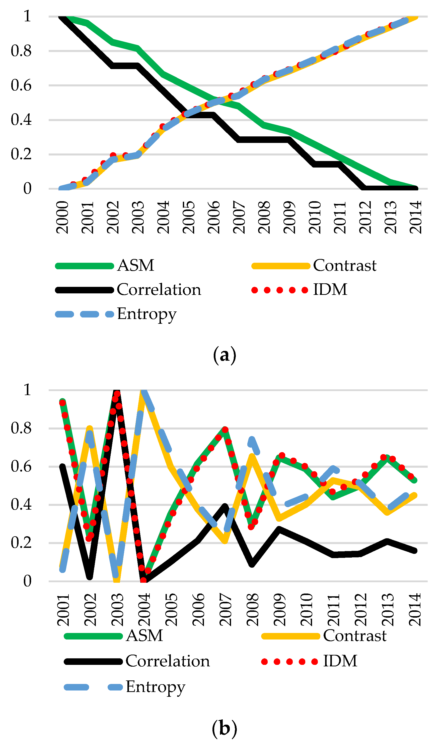
Figure 6 shows the spatiotemporal evolution of fractal indices in standardized values for the total deforested areas. As the extent of deforestation increased during the analyzed period, the fractal textural complexity of total deforested areas from Curvature Carpathians increased from 2001 to 2014 indicating that the deforestation was done chaotically. FFI of total deforested areas from Curvature Carpathians has diminished because of the growth of deforested land between 2000 and 2014, indicating a continuous increase in fragmentation of the tree cover areas (Table A1).

Until 2004, a tendency of increasing clustering, from 0.002 to 0.01 was observed. FFI of the regenerated areas for the period 2001–2014 was very small, only 0.004 higher than the deforested areas. This fact indicates that the regeneration was accomplished more compactly than the deforestation, even if the deforestation was lower. ${\Lambda }_{T-o-W}$ of regenerated areas was smaller than that of deforested areas, except where the tree cover canopy was between 60–100% (where the forest was more compact, the regeneration was lower than defrosting and made less compact) (Figure 7).

As the extent of deforestation increased during the analyzed period, Pyramid and Cube Dimensions of the Curvature Carpathian total deforested areas increased from 2001 to 2014, indicating that the deforestation was done in a chaotically manner (Figure 7). The values of Pyramid Dimension and Cube Counting of the regenerated area for 2001–2014 were lower than of the deforested area, indicating that regeneration was rather even.

3.2. GLCM Analysis

Figure 8a–c shows that the GLCM analysis provided information like the fractal texture complexity analysis obtained through Pyramid Dimension and Cube Counting. The GLCM analysis directly correlated with fractal textural complexity analysis through Entropy and Contrast and vice versa through Correlation, IDM and ASM. Thus, as the textural fractal complexity increases, the clutter increases—entropy, contrast and IDM, but uniformity and correlation decrease. GLCM confirmed that significant changes in the matrix occurred in years with more intense, homogeneous, compact deforestation (2002, 2004, 2005 and 2008) and less significant changes in years with more heterogeneous fragmented deforestation (2001, 2003 and 2007). It was also confirmed that regenerated areas in the 2001–2014 period were relatively evenly distributed when compared to deforestation.

Correlation, which represents the linear dependence of grey tones, had slightly different results compared to the other GLCM indices. The differences were more obvious for deforested areas and total deforested areas. In the total deforested areas, the linear dependence of grey tones has fallen sharply, followed by a flat region due to clustering of deforestation. Corresponding data is found in

Table A2. Values of GLCM indices.

	ASM	Contrast	Correlation	IDM	Entropy
Tree Cover Areas
2000	0.4432	1286.099	8.91 × 10−5	0.7482	2.6264
2001	0.4431	1298.898	8.90 × 10−5	0.748	2.6288
2002	0.4428	1345.123	8.89 × 10−5	0.7475	2.637
2003	0.4427	1353.752	8.89 × 10−5	0.7475	2.6386
2004	0.4423	1406.954	8.88 × 10−5	0.7469	2.6479
2005	0.4421	1438.549	8.87 × 10−5	0.7466	2.6538
2006	0.4419	1460.727	8.87 × 10−5	0.7464	2.6577
2007	0.4418	1475.708	8.86 × 10−5	0.7462	2.6603
2008	0.4415	1505.495	8.86 × 10−5	0.7459	2.6661
2009	0.4414	1525.111	8.86 × 10−5	0.7457	2.6696
2010	0.4412	1546.474	8.85 × 10−5	0.7455	2.6734
2011	0.441	1569.874	8.85 × 10−5	0.7453	2.6779
2012	0.4408	1593.624	8.84 × 10−5	0.745	2.682
2013	0.4406	1614.046	8.84 × 10−5	0.7448	2.6853
2014	0.4405	1636.108	8.84 × 10−5	0.7446	2.689
Deforested Areas
2001	0.9992	14.7521	0.02862	0.9996	0.005225
2002	0.9968	54.9259	0.007965	0.9985	0.01852
2003	0.9994	10.3896	0.04297	0.9997	0.004077
2004	0.996	66.1101	0.00713	0.9982	0.02274
2005	0.9972	43.8244	0.01083	0.9987	0.01652
2006	0.9981	31.4481	0.01477	0.9991	0.01157
2007	0.9987	22.1769	0.02118	0.9994	0.008401
2008	0.997	46.7975	0.01031	0.9986	0.01795
2009	0.9982	28.7583	0.01692	0.9992	0.01129
2010	0.998	32.8301	0.01463	0.9991	0.01236
2011	0.9975	39.7488	0.01211	0.9989	0.0151
2012	0.9977	37.9728	0.01226	0.999	0.01365
2013	0.9982	30.4681	0.01465	0.9992	0.01107
2014	0.9978	35.4677	0.01288	0.999	0.01307
Total Deforested Areas
2001	0.9992	14.7521	0.02862	0.9996	0.005225
2001–2002	0.996	68.8795	0.006385	0.9982	0.02272
2001–2003	0.9954	78.7414	0.005634	0.9979	0.02589
2001–2004	0.9916	140.6398	0.003326	0.9962	0.04544
2001–2005	0.989	178.5612	0.002678	0.995	0.05845
2001–2006	0.9872	204.7712	0.002356	0.9942	0.06698
2001–2007	0.986	222.8843	0.002176	0.9937	0.07293
2001–2008	0.9833	258.9493	0.001898	0.9925	0.08617
2001–2009	0.9816	281.5754	0.001754	0.9918	0.09407
2001–2010	0.9798	307.1283	0.001614	0.991	0.1027
2001–2011	0.9776	335.9417	0.001481	0.9901	0.1131
2001–2012	0.9755	364.6361	0.001366	0.9892	0.1224
2001–2013	0.9739	389.0011	0.00128	0.9885	0.1298
2001–2014	0.972	415.5841	0.001199	0.9876	0.1384

. GLCM analysis confirmed that significant changes in the matrix occurred in years with more intense, homogeneous, compact deforestation (2002, 2004, 2005 and 2008) and less significant changes in years with more heterogeneous fragmented deforestations (2001, 2003 and 2007).

4. Discussion and Conclusions

Mapping the forest dynamics as the main objective of this study was carried out using multiple fractal and GLCM indices.

Table 1. Statistical summary of deforested areas/total deforested areas/tree cover areas (ha.) from 2001 to 2014 [33]. ¹ the highest value of deforested areas; ² total deforested areas; ³ the highest value of tree cover areas.

Year/Class	Deforested Areas	Total Deforested Areas	Tree Cover Areas
2001	341.15	341.15	388,458.52 3
2002	1324.53	1665.69	387,133.99
2003	260.97	1926.66	386,873.01
2004	1715.83 1	3642.49	385,157.18
2005	1189.94	4832.43	383,967.24
2006	811.47	5643.91	383,155.77
2007	576.89	6220.80	382,578.88
2008	1293.22	7514.01	381,285.66
2009	806.02	8320.03	380,479.64
2010	864.90	9184.93	379,614.74
2011	1062.21	10,247.14	378,552.53
2012	971.15	11,218.29	377,581.38
2013	754.94	11,973.23	376,826.44
2014	927.20	12,900.43 2	375,899.24

shows the main results for the deforested areas (as deforested areas for each year), total deforested areas (as cumulative deforested areas, obtained by cumulating the deforested areas for each year) and tree cover areas, from 2001 to 2014. In 2007 and 2012 the most pronounced annual average deforestation and forest area minimums were registered in 2003 and 2014, due to changes in deforestation politics which increased the permissiveness of the forest code. It is interesting to notice that the highest values of deforested areas were recorded in 2004 and 2008 when forest dynamics was influenced by legislative modifications through the law 247/2005 [45] and significant political changes. The Romanian Forestry Policy changed by introducing regulations for logging and timber harvesting, but these have not resulted in sustainable protection of forests.

The evolution of the tree cover areas of the Curvature Carpathians in the period 2000–2014 revealed a general trend of decline, caused by legal and illegal logging. This situation was a consequence of the economic and legislation changes resulting in increased deforestation [16,19,20,21]. In this study, we used fractal and GLCM analysis to study the evolution of the degree of heterogeneity and dispersion of deforested areas, total deforested areas and tree cover areas. The obtained results indicate that:

(1)

The tree cover areas have diminished as deforestation increases;

(2)

The clustering increases by deforestation (by increasing compaction and homogenization), especially after 2005;

(3)

Deforestation was made less compact than regeneration, although the areas were smaller;

(4)

The use of Pyramid Dimension allowed us to quantify the degree of textural complexity imposed by deforestation on tree cover areas;

(5)

The use of the Cube Counting Dimension allowed us to quantify the degree of textural complexity imposed by deforestation on tree cover areas through a 3D analysis;

(6)

GLCM analysis confirmed the fractal analysis, indicating that the link of uniformity/non-uniformity between neighboring pixels reflects the complexity of pixel relationships obtained by Pyramid Dimension and Cube Counting;

(7)

3D fractal analysis reveals an added value to classical 1D and 2D fractal analyses by enabling the analysis of the complete set of data through a single fractal value;

(8)

${\Lambda }_{T-o-W}$ revealed the local effects of deforestation on the compaction of the tree cover areas. In this regard, we show that in years with more homogeneous, compact and more intense deforestation ${\Lambda }_{T-o-W}$ indicated that deforestation has accentuated the process to heterogenization of the tree cover areas. In years with more heterogeneous, fragmented deforestation${\Lambda }_{T-o-W}$ indicated that deforestation had limited effects on the compaction of tree cover areas;

(9)

In the years with minimum deforestation, FFI should have low values, close to 0, but there are also special situations, as in 2002, when the FFI, the FFI had very low values, even the deforested areas were very large (1324.5 hectares). This was due to deforestation dominated by small and numerous petitions. So, FFI captures the deforestation” behavior” better than area analysis, fractal or classical GLCM analysis.

(10)

Regeneration has become more heterogeneous and fragmented than deforestation.

This is the first time that Pyramid Dimension and Cube Counting are analyzed for the study of forests. GLCM has also been used in the analysis of forests in the Central Group of Eastern Carpathians in Romania [46]. Compared to the previous study, our results showed that the degree of forest and deforestation disorder in the Curvature Carpathians is higher than that of the Central Group.

In terms of fractal fragmentation of forests, Curvature Carpathians has proved to be more compact than the Northern Carpathian Mountains [47], Central Carpathians [46] Apuseni Mountains [32], but more fragmented than Bucegi Group [48].

Regarding ${\Lambda }_{T-o-W}$, the spatial distribution of forests in the southern group proved to be more homogeneous than in the situation of the Northern Carpathian Mountains, Central Carpathians and Apuseni Mountains [32,47].

Our study has some limitations that need to be addressed. The images used, with a spatial resolution of 30 m, allowed us to capture only a coarser image of the forest models. The use of more detailed images would solve this restriction and thus improve the accuracy of fractal and GLCM analyzes. For a correct analysis all the analyzed images must have the same resolution, and the gray tones have the same characteristics for all the images.

Our findings confirm our hypothesis that fractal analysis on Landsat images from GFC, with a 30 m spatial resolution, provides valuable quantitative information on the spatiotemporal patterns of deforestation and forest areas. Thus, through fractal analysis, we have obtained complementary information on deforestation compared to classical image analysis based on image classification, because fractal analysis is able to analyze irregular spatial structures.

In conclusion, the forest change detection at a 30 m spatial resolution from GFC has helped to get a spatial and temporal dimension of forest cover change. The fractal and GLCM indices confirmed the high rate of deforestation and fragmentation of forest ecosystems from Curvature Carpathians. The trend of deforestation follows a continuous growth and causes instability of forest components and is thus unsustainable.

References

1. Munteanu, C.; Niță, M.D.; Abrudan, L.V.; Radeloff, V.C. Historical forest management in Romania is imposing strong legacies on contemporary forests and their management. For. Ecol. Manag. 2016, 361, 179–193. [Google Scholar] [CrossRef]
2. Ginesu, S.; Carboni, D.; Marin, M. Erosion and use of the coast in the northern Sardinia (Italy). Procedia Environ. Sci. 2016, 32, 230–243. [Google Scholar] [CrossRef] [Green Version]
3. Zajac, S.; Kaliszewski, A.; Mlynarski, W. Forests and forestry in Poland and other EU countries. Folia For. Pol. 2014, 56, 185–193. [Google Scholar] [CrossRef] [Green Version]
4. Seidl, R.; Rammer, W.; Jager, D.; Currie, W.S.; Lexer, M.J. Assessing trade-offs between carbon sequestration and timber production within a framework of multi-purpose forestry in Austria. For. Ecol. Manag. 2007, 248, 64–79. [Google Scholar] [CrossRef]
5. Nedelea, A.; Comănescu, L.; Oprea, R. The ecoclimatic indexes specific for the Argeș valley (Făgăraș Mountains, the Southern Carpathians, Romania). Int. J. Phys. Sci. 2009, 4, 796–805. [Google Scholar]
6. Budeanu, M.; Petritan, A.M.; Popescu, F.; Vasile, D.; Tudose, N.C. The Resistance of European Beech (Fagus sylvatica) from the Eastern Natural Limit of Species to Climate Change. Not. Bot. Horti Agrobot. Cluj-Napoca 2016, 44, 625–633. [Google Scholar] [CrossRef] [Green Version]
7. Griffiths, P.; Kuemmerle, T.; Kennedy, R.E.; Abrudan, I.V.; Knorn, J.; Hostert, P. Using annual time-series of Landsat images to assess the effects of forest restitution in post-socialist Romania. Remote Sens. Environ. 2010, 118, 199–214. [Google Scholar] [CrossRef]
8. Brus, D.J.; Hengeveld, G.M.; Walvoort, D.J.J.; Goedhart, P.W.; Heidema, A.H.; Nabuurs, G.J.; Gunia, K. Statistical mapping of tree species over Europe. Eur. J. For. Res. 2012, 131, 145–157. [Google Scholar] [CrossRef]
9. Abrudan, I.V. A decade of non-state administration of forests in Romania: Achievements and challenges. Int. For. Rev. 2012, 14, 275–284. [Google Scholar] [CrossRef]
10. Food and Agriculture Organization of United Nations (FAO) Report. Available online: http://www.fao.org/docrep/w7170E/w7170e0f.htm (accessed on 4 May 2019).
11. Romanescu, G.; Mihu-Pintilie, A.; Stoleriu, C.C.; Carboni, D.; Paveluc, L.E.; Cimpianu, C.I. A Comparative Analysis of Exceptional Flood Events in the Context of Heavy Rains in the Summer of 2010: Siret Basin (NE Romania) Case Study. Water 2018, 10, 216. [Google Scholar] [CrossRef] [Green Version]
12. Stăncioiu, P.T.; Abrudan, I.V.; Dutca, I. The Natura 2000 ecologicalnetworkandforests in Romania: Implications on management and administration. Int. For. Rev. 2010, 12, 106–113. [Google Scholar] [CrossRef]
13. WWF Global. Available online: http://wwf.panda.org/who_we_are/wwf_offices/romania/?224930/WWF-supports-beech-virgin-forests-in-Romania-to-become-part-of-the-UNESCO-World-Heritage-list (accessed on 4 May 2017).
14. Parviainen, J. Virgin and natural forests in the temperate zone of Europe. For. Snow Landsc. Res. 2005, 79, 9–18. [Google Scholar]
15. Constandache, C.; Blujdea, V. Achievements and Perspectives on the Improvement by Afforestation of Degraded Lands in Romania. In Proceedings of the 5th International Conference on Land Degradation, Bari, Italy, 18–22 September 2009; Springer: Berlin, Germany, 2010; pp. 547–560. [Google Scholar]
16. Pintilii, R.D.; Andronache, I.; Diaconu, D.C.; Dobrea, R.C.; Zeleňáková, M.; Fensholt, R.; Peptenatu, D.; Draghici, C.C.; Ciobotaru, A.M. Using Fractal Analysis in Modeling the Dynamics of Forest Areas and Economic Impact Assessment: Maramureș County, Romania, as a Case Study. Forests 2017, 8, 25. [Google Scholar] [CrossRef] [Green Version]
17. Andronache, I.; Fensholt, R.; Ahammer, H.; Ciobotaru, A.M.; Pintilii, R.D.; Peptenatu, D.; Drăghici, C.C.; Diaconu, D.C.; Radulovic, M.; Pulighe, G.; et al. Assessment of Textural Differentiations in Forest Resources in Romania Using Fractal Analysis. Forests 2017, 8, 54. [Google Scholar] [CrossRef] [Green Version]
18. Griffiths, P.; Kuemmerle, T.; Baumann, M.; Radeloff, V.C.; Abrudan, I.V.; Lieskovsky, J.; Munteanu, C.; Ostapowicz, K.; Hostert, P. Forest disturbances, forest recovery, and changes in forest types across the Carpathian ecoregion from 1985 to 2010 based on Landsat image composites. Remote Sens. Environ. 2014, 151, 72–88. [Google Scholar] [CrossRef]
19. Pintilii, R.D.; Papuc, R.M.; Drăghici, C.C.; Simion, A.G.; Ciobotaru, A.M. The Impact of Deforestation on The Structural Dynamics of Economic Profile in The Most Affected Territorial Systems in Romania. In Proceedings of the 15th International Multidisciplinary Scientific Geoconference (SGEM), Albena, Bulgaria, 18–24 June 2015; Stef92 Technology Ltd.: Sofia, Bulgaria, 2015; pp. 567–573. [Google Scholar]
20. Andronache, I.; Ahammer, H.; Jelinek, H.F.; Peptenatu, D.; Ciobotaru, A.M.; Drăghici, C.C.; Pintilii, R.D.; Simion, A.G.; Teodorescu, C. Fractal analysis for studying the evolution of forests. Chaos Solitons Fractals 2016, 91, 310–318. [Google Scholar] [CrossRef]
21. Ciobotaru, A.M.; Peptenatu, D.; Andronache, I.; Simion, A.G. Fractal characteristics of the afforested, deforested and reforested areas in Suceava county, Romania. In Proceedings of the International Scientific Conferences on Earth & Geo Sciences—Sgem Vienna Green Sessions 2016, Viena, Austria, 2–5 November 2016; Stef92 Technology Ltd.: Sofia, Bulgaria, 2016; pp. 445–452. [Google Scholar]
22. Vorovencii, I.; Ienciu, I.; Oprea, L.; Popescu, C. Identification of Illegal Loggings inHarghita Mountains, Romania, Using Landsat Satellite Images. In Proceedings of the 13th International Multidisciplinary Scientific Geoconference, SGEM, Albena, Bulgaria, 16–22 June 2013; Stef92 Technology Ltd.: Sofia, Bulgaria, 2013; pp. 609–616. [Google Scholar]
23. Griffiths, P.; Hostert, P. Forest Cover Dynamics During Massive Ownership Changes—Annual Disturbance Mapping Using Annual Landsat Time-Series. In Remote Sensing Time Series. Remote Sensing and Digital Image Processing; Kuenzer, C., Dech, S., Wagner, W., Eds.; Springer: Dordrecht, The Netherlands, 2015; Volume 22, pp. 307–322. [Google Scholar]
24. Strîmbu, B.M.; Hickey, G.M.; Strîmbu, V.G. Forest conditions and management under rapid legislation change in Romania. For. Chron. 2005, 81, 350–358. [Google Scholar] [CrossRef]
25. Petritan, A.M.; Nuske, R.S.; Petritan, I.C.; Tudose, N.C. Gap disturbance patterns in an old-growth sessile oak (Quercus petraea L.)-European beech (Fagus sylvatica L.) forest remnant in the Carpathian Mountains, Romania. For. Ecol. Manag. 2013, 308, 67–75. [Google Scholar] [CrossRef]
26. Svoboda, M.; Janda, P.; Bace, R.; Fraver, S.; Nagel, T.A.; Rejzek, J.; Mikolas, M.; Douda, J.; Boublik, K.; Samonil, P.; et al. Landscape-level variability in historical disturbance in primary Piceaabies mountain forests of the Eastern Carpathians, Romania. J. Veg. Sci. 2014, 25, 386–401. [Google Scholar] [CrossRef]
27. Pop, I.M.; Sallay, A.; Bereczky, L.; Chiriac, S. Land use and behavioral patterns of brown bears in the South-Eastern Romanian Carpathian Mountains: A case study of relocated and rehabilitated individuals. In Proceedings of the 2011 International Conference of Environment-Landscape-European Identity, Bucharest, Romania, 4–6 November 2011; Elsevier Science Bv: Amsterdam, The Netherlands, 2012; pp. 111–122. [Google Scholar]
28. Blaj, R.; Sand, C.; Stanciu, M.; Antonie, I. Consideration Regarding the Forest Importance in The Sustainable Development. In Proceedings of the 18th International Conference—The Knowledge-Based Organization: Applied Technical Sciences and Advanced Military Technologies, Conference Proceeding 3, Sibiu, Romania, 14–16 June 2012; Nicolae Bălcescu-Land Forces Academy: Sibiu, Romania, 2012; pp. 169–173. [Google Scholar]
29. Moatar, M.; Fora, C.; Banu, C.; Ștefan, C.; Stanciu, S. Researches Concerning Installing Forest Vegetation on Degraded Lands. In Proceedings of the 15th International Multidisciplinary Scientific Geoconference (SGEM), Albena, Bulgaria, 18–24 June 2015; Stef92 Technology Ltd.: Sofia, Bulgaria, 2015; pp. 521–527. [Google Scholar]
30. Comănescu, L.; Nedelea, A. Public perception of the hazards affecting geomorphological heritage-case study: The central area of Bucegi Mts. (Southern Carpathians, Romania). Environ. Earth Sci. 2015, 73, 8487–8497. [Google Scholar] [CrossRef]
31. National Institute of Statistics, Romania. Available online: http://statistici.insse.ro:8077/tempo-online/ (accessed on 30 April 2017).
32. Andronache, I.; Marin, M.; Fischer, R.; Ahammer, H.; Radulovic, M.; Ciobotaru, A.M.; Jelinek, F.H.; Di Ieva, A.; Pintilii, R.D.; Drăghici, C.C.; et al. Dynamics of Forest Fragmentation and Connectivity Using Particle and Fractal Analysis. Sci. Rep. 2019, 9, 12228. [Google Scholar] [CrossRef] [PubMed] [Green Version]
33. Hansen, M.C.; Potapov, P.V.; Moore, R.; Hancher, M.; Turubanova, S.A.; Tyukavina, A.; Thau, D.; Stehman, S.V.; Goetz, S.J.; Loveland, T.R.; et al. High-resolution global maps of 21st-century forest cover change. Science 2013, 342, 850–853. [Google Scholar] [CrossRef] [PubMed] [Green Version]
34. Kainz, P.; Mayrhofer-Reinhartshuber, M.; Ahammer, H. IQM: An Extensible and Portable Open Source Application for Image and Signal Analysis. PLoS ONE 2015, 10, e0116329. [Google Scholar] [CrossRef] [PubMed] [Green Version]
35. Nečas, D.; Klapetek, P. Gwyddion: An open-source software for SPM data analysis. Cent. Eur. J. Phys. 2012, 10, 181–188. [Google Scholar] [CrossRef]
36. Mayrhofer-Reinhartshuber, M.; Ahammer, H. Pyramidal fractal dimension for high resolution images. Chaos 2016, 26, 7. [Google Scholar] [CrossRef]
37. Ahammer, H.; Andronache, I. IQM-Plugin-FFI 2016–2017. Available online: https://sourceforge.net/projects/iqm-plugin-frac2d/ (accessed on 6 January 2017).
38. Reiss, M. IQM Plugin frac2D. 2016. Available online: https://sourceforge.net/projects/iqm-plugin-ffi/ (accessed on 30 April 2017).
39. Haralick, R.M.; Shanmugam, K.; Dinstein, I. Texture parameters for image classification. IEEE Trans. Syst. Man Cybern. 1973, SMC-3, 610–621. [Google Scholar] [CrossRef] [Green Version]
40. Cornish, T.B. GLCM_TextureToo 2017. Available online: http://tobycornish.com/downloads/imagej/ (accessed on 14 February 2018).
41. Djuricic, G.J.; Radulovic, M.; Sopta, J.P.; Nikitovic, M.; Milosevic, N.T. Fractal and Gray Level Cooccurrence Matrix Computational Analysis of Primary Osteosarcoma Magnetic Resonance Images Predicts the Chemotherapy Response. Front. Oncol. 2017, 7. [Google Scholar] [CrossRef] [Green Version]
42. Arivazhagan, S.; Ganesan, L.; Padam Priyal, S. Texture classification using Gabor wavelets-based rotation invariant features. Pattern Recognit. Lett. 2006, 27, 1976–1982. [Google Scholar] [CrossRef]
43. Meng, S.; Pang, Y.; Zhang, Z.; Jia, W.; Li, Z. Mapping Above-ground Biomass using Texture Indices from Aerial Photos in the Temperate Forest of Northeastern China. Remote Sens. 2016, 8, 230. [Google Scholar] [CrossRef] [Green Version]
44. Proisy, C.; Couteron, P.; Fromard, F. Predicting and mapping mangrove biomass from canopy grain analysis using Fourier-based textural ordination of IKONOS images. Remote Sens. Environ. 2007, 109, 379–392. [Google Scholar] [CrossRef]
45. Romanian Government Official Monitor. Law no. 247/2005 on the Reform of Property and Justice, as Well as Some Accompanying Measures. Available online: http://legislatie.just.ro/Public/DetaliiDocument/63447 (accessed on 24 April 2019).
46. Ciobotaru, A.M.; Andronache, I.; Ahammer, H.; Jelinek Herbert, F.; Radulovic, M.; Pintilii, R.D.; Peptenatu, D.; Drăghici, C.C.; Simion, A.G.; Papuc, R.M.; et al. Recent Deforestation Pattern Changes (2000–2017) in the Central Carpathians: A Gray-Level Co-Occurrence Matrix and Fractal Analysis Approach. Forests 2019, 10, 308. [Google Scholar] [CrossRef] [Green Version]
47. Drăghici, C.C.; Andronache, I.; Ahammer, H.; Peptenatu, D.; Pintilii, R.D.; Ciobotaru, A.M.; Simion, A.G.; Dobrea, R.C.; Diaconu, D.C.; Vişan, M.C.; et al. Spatial evolution of forest areas in the northern Carpathian Mountains of Romania. Acta Montan. Slovaka 2017, 22, 95–106. [Google Scholar]
48. Diaconu, D.C.; Andronache, I.; Pintilii, R.D.; Bretcan, P.; Simion, A.G.; Draghci, C.C.; Gruia, A.K.; Grecu, A.; Marin, M.; Peptenatu, D. Using Fractal Fragmentation and Compaction Index in Analysis of the Deforestation Process in Bucegi Mountains Group, Romania. Carpathian J. Earth Environ. Sci. 2019, 14, 431–438. [Google Scholar] [CrossRef]
Figure 1. (a) The study area; (b) Deforestation in the study area (2000–2014) [33].
Sustainability 11 06927 g001
Figure 2. Flowchart of mapping forest changes in Curvature Carpathians using GLCM and Fractal Analysis.
Sustainability 11 06927 g002
Figure 3. Evolution of fractal indices (standardized values) for the period 2000–2014. Pyramid Dimension (R2 = 0.9922), Cube Counting Dimension (R2 = 0.8187), FFI (R2 = 0.9741) and Λ T o W (R2 = 0.3264). R2 is the coefficient of determination.
Sustainability 11 06927 g003
Figure 4. Evolution of fractal indices (standardized values) for the period 2000-2014. Pyramid Dimension (R2 = 0.0059), Cube Counting Dimension (R2 = 0.0527), FFI (R2 = 0.1409) and Λ T o W (R2 = 0.147). R2 is the coefficient of determination.
Sustainability 11 06927 g004
Figure 5. Evolution of Λ T o W in function of tree cover canopy (absolute values).
Sustainability 11 06927 g005
Figure 6. Evolution of fractal indices (standardized values) related to total deforested areas for 2000–2014. Pyramid Dimension (R2 = 0.0963), Cube Counting Dimension (R2 = 0.7544), FFI (R2 = 0.9561) and Λ T o W (R2 = 0.7918). R2 is the coefficient of determination.
Sustainability 11 06927 g006
Figure 7. Λ T o W   of deforested and reforested areas, by the degree of tree cover canopy.
Sustainability 11 06927 g007
Figure 8. (a) Evolution of GLCM indices (standardized values) for 2000-2014 for tree cover areas. ASM (R2 = 0.9938), Contrast (R2 = 0.9902), Correlation (R2 = 0.9588), IDM (R2 = 0.9887) and Entropy (R2 = 0.9902); (b) for deforested areas: ASM (R2 = 0.0025), Contrast (R2 = 0.0003), Correlation (R2 = 0.1214), IDM (R2 = 1 × 10⁻²⁷) and Entropy (R2 = 0.0054); (c) for total deforested areas: ASM (R2 = 0.9948), Contrast (R2 = 0.9894), Correlation (R2 = 0.3677), IDM (R2 = 0.9934) and Entropy (R2 = 0.9913). R2 is the coefficient of determination.
Sustainability 11 06927 g008aSustainability 11 06927 g008b