Random Spatial and Systematic Random Sampling Approach to Development Survey Data: Evidence from Field Application in Malawi

Abstract

Implementing development surveys in developing countries can be challenging. Limited time, high survey costs, lack of information, and technical difficulties are some of the general constraints that plague development researchers. These constraints can hinder data collection and introduce selection bias into the survey data. We outline a multilevel sampling approach for use in areas where comprehensive information on geographical or household characteristics of local population are not readily available. Our approach includes the use of geographical information systems (GIS) for random spatial sampling and personal digital assistants (PDAs) with a global positioning system (GPS) for household systematic random sampling with random walk. Evidence from our field application in Malawi show that the multilevel sampling approach yields relevant survey data which is comparable to historical and nationally representative values; and supports rapid aggregation of preliminary results after the survey. This multilevel design is cost-effective in implementation and reduces bias avenues in the household selection. Overall, this multilevel sampling approach can be used to generate survey data in developing countries where detailed geographical information and household characteristics data are not readily available. It also presents ways of reducing bias in survey data given budget constraints.

1. Introduction

Household survey sampling is vital to development research. In the agricultural and development context, researchers use household surveys to collect information on farming cycles, land use, and crop harvests. In addition to resource use, information on household socio-economic and social demographic characteristics can influence development patterns and thus, is vital to village policy decisions especially for sustainable resource management [1,2]. As a result, development survey may use spatial sampling to extract information on household economic and social characteristics as well as information on natural resource use like land or forestry.

Spatial sampling is essential to development studies. Researchers use several spatial characteristics to assess the social and economic conditions of target population [3,4]. Because it is difficult to sample every population frame, such as households or individuals, in most studies, researchers must resort to different sampling techniques to capture representative and relevant data [3,5]. This sampling difficulty is exacerbated in developing or resource-constrained settings where it is challenging to obtain accurate and up-to-date geographic or household data [3]. In rural areas, household geographic data are mostly informal, irregular or even completely absent compared to developed settings, and as a result, place severe constraints on survey sampling design and create measurement errors in the final survey data [5,6]. For researchers, it is pertinent to find sampling methodologies which can derive relevant results in these conditions. High quality nationally representative surveys like the Demographic and Household Surveys (DHS) use sampling methods that are time-consuming and expensive, and thus, not suitable for smaller or budget-constrained research. In population studies, cluster sampling is the most common method used to obtain representative data [3,7], mostly implemented as a two-stage cluster sampling design. In the first stage, census enumeration is used to identify the primary sampling units while in the second stage, sampled households are selected from a household unit listing respectively [8]. While accurate household unit listings in developing countries are costly to compile, researchers seeking to obtain comparable data in budget-constrained studies could use multistage sampling to reduce the number of sampling sites and techniques like random spatial sampling to reduce the chances of sampling bias in the survey data [8]. Random spatial sampling uses sample frames containing identifiable geographic units. The geographic units are selected randomly using a spatial sampling software and seek to capture the estimated variable of interest within a minimum number of sampling sites [9].

Spatial sampling methods using geographic information systems (GIS) are being increasingly adopted in a broad range of research applications, such as for air pollution, climate, agriculture, land use, and population studies [9,10,11,12,13]. It is also increasingly combined with other technologies like personal digital assistants (PDAs) and global positioning systems (GPS) for in-field data collection. The use of PDAs, GIS and GPS in social sciences ranges from research applications in land management and health analysis, to socio-economic and agricultural analysis [4,9,14,15,16]. GIS and GPS involve hardware, software and geographical data which, when combined, provide users with geographical information of a particular space/place as well as satellite navigation services [14]. PDA use for data collection in combination with GIS location services or GPS-generated sampling frames are been documented extensively in development and social science research [3,4].

Further research in other domains of social sciences show that combining random spatial sampling with GIS, GPS or PDA technology can support effective survey sampling and data aggregation. For example, Himelein et al. [8] outline a random geographic cluster (RGC) sampling design using GIS and GPS technology as key to capturing representative livestock household data from a nomadic population in the Afar region of Ethiopia. Using stratified random spatial sampling on high spatial resolution Earth data, Brink and Eva [15] show the increasing negative impact of agricultural intensification on natural vegetation in sub-Saharan Africa. The use of GIS and GPS is also been noted extensively in population studies. For instance, Kondo et al. [3] show that stratified random sampling method with GIS and GPS technology could reduce selection bias in population data in resource-constrained scenarios. Similarly, Grais et al. [16] show that the sample grid method with a random starting point using GPS provides the fastest and easiest method for data collection for field survey teams and is a quicker and more robust alternative to the traditional “spinning the pen” method. Finally, Shirima et al. [17] highlight the time-saving and enhanced data quality properties gotten from using PDAs for data entry at the point of collection in scattered rural households in Tanzania.

This article describes a multilevel sampling approach, suitable for survey areas where comprehensive information on geographical or household characteristics and local population data is not readily available. Our article builds on previous research on spatial and systematic random sampling as well as the use of multilevel survey design in developing countries using GIS and GPS technology, thus, contributing to the literature surrounding these topics. First, we use geographical information systems (GIS) with random spatial sampling to generate spatial sampling units. Second, we use personal digital assistants (PDAs) with a global positioning system (GPS) for household systematic random sampling with random walk to generate relevant data for women farmers in Malawi.

The next sections describe our multilevel sampling design, the required field sample estimation and field implementation. Finally, we leverage field survey teams’ feedback, interviewer performance indicators from our field results and the comparison of a key variable of interest to explore; and conclude on issues surrounding the preparations and limitations of our sampling approach.

2. Methods

2.1. General Research Aim

Our primary research objective for Malawi was to collect information on indicators of human recognition—an intangible novel concept of human development and a key variable of interest (see

Table 1. Domains of negative human recognition and indicators.

Domain	Domain Indicators	Malawi DHS	Primary Data
Self (1)	Person with …
	usually decides on respondent’s health care.	X	X
	usually decides on visits to respondent’s family/relatives.	X	X
	usually decides on household purchases.	X	X
	Beating justified if … wife goes out without telling spouse/partner	X	X
	wife neglects children	X	X
	wife goes argues with spouse/partner	X	X
	wife refuses to have sex with spouse/partner	X	X
	wife burns food	X	X
	wife is unfaithful		X
	wife is disrespectful		X
Household (2)	Spouse/partner…
	doesn’t spend his free time with respondent.		X
	doesn’t consult respondent on different household matters		X
	is not affectionate with respondent		X
	does not respect respondent or respondent’s wishes		X
	jealous if respondent talks with other men	X	X
	accuses respondent of unfaithfulness	X	X
	doesn’t permit respondent to meet with female friends	X	X
	tries to limit respondent’s contact with family	X	X
	insists on knowing where respondent is	X	X
	Respondent has been… humiliated, threatened with harm, insulted or made to feel bad by spouse/partner	X	X
	pushed, shook, had something thrown at, slapped, punched with a fist or hit by something harmful, had arm twisted or hair pulled by spouse/partner	X	X
	kicked or dragged, strangled or burnt, threatened with knife/gun or another weapon by spouse/partner.	X	X
	physically forced to perform sexual acts respondent didn’t want to.	X	X
	has ever had physical injuries because of spouse/partner actions	X	X
	hurt spouse/partner during a pregnancy.	X
Community (3)	Someone else … physically hurt respondent in the community.	X	Xa
	respondent during pregnancy in the community.	X
	Respondent has experienced beating, verbal or emotional violence from other family members and community leaders or officials		X

Source. Malawi DHS [22], Authors’ own; Notes: indicators marked “X” are available in both datasets; “X^a”—indicator also includes during pregnancy.

)—as well as socio-economic and social demographic data (household characteristics, employment and labor force participation, land use, agriculture, consumption, and investment habits) from women famers at the household level. Particularly, Castleman [18,19] defines human recognition as “[…] the acknowledgement provided to an individual by other individuals, groups, or organizations that the individual is of inherent value with intrinsic qualities in common with the recognizer, i.e. acknowledgement as a fellow human being […]”. In other words, human recognition address how individuals are viewed, valued and treated by others in society with significant influence on their wellbeing. According to Castleman [18], positive or negative human recognition provided in recipients’ sphere of interaction, that is negative/positive human recognition in the self, household and community domains, can exert significant effects on the material wellbeing of its recipients. Because human recognition can lead to changes in empowerment, dignity and poverty, which in turn, affect the utility and wellbeing of its recipients, we note that the impact of human recognition on women farmer’s wellbeing is obscured if factors influencing negative/positive human recognition provision are not identified [20,21]. We argue that if negative/positive human recognition exists in a target population of women farmers, it should be detectible within a sub-sample of the target population, examined in the field.

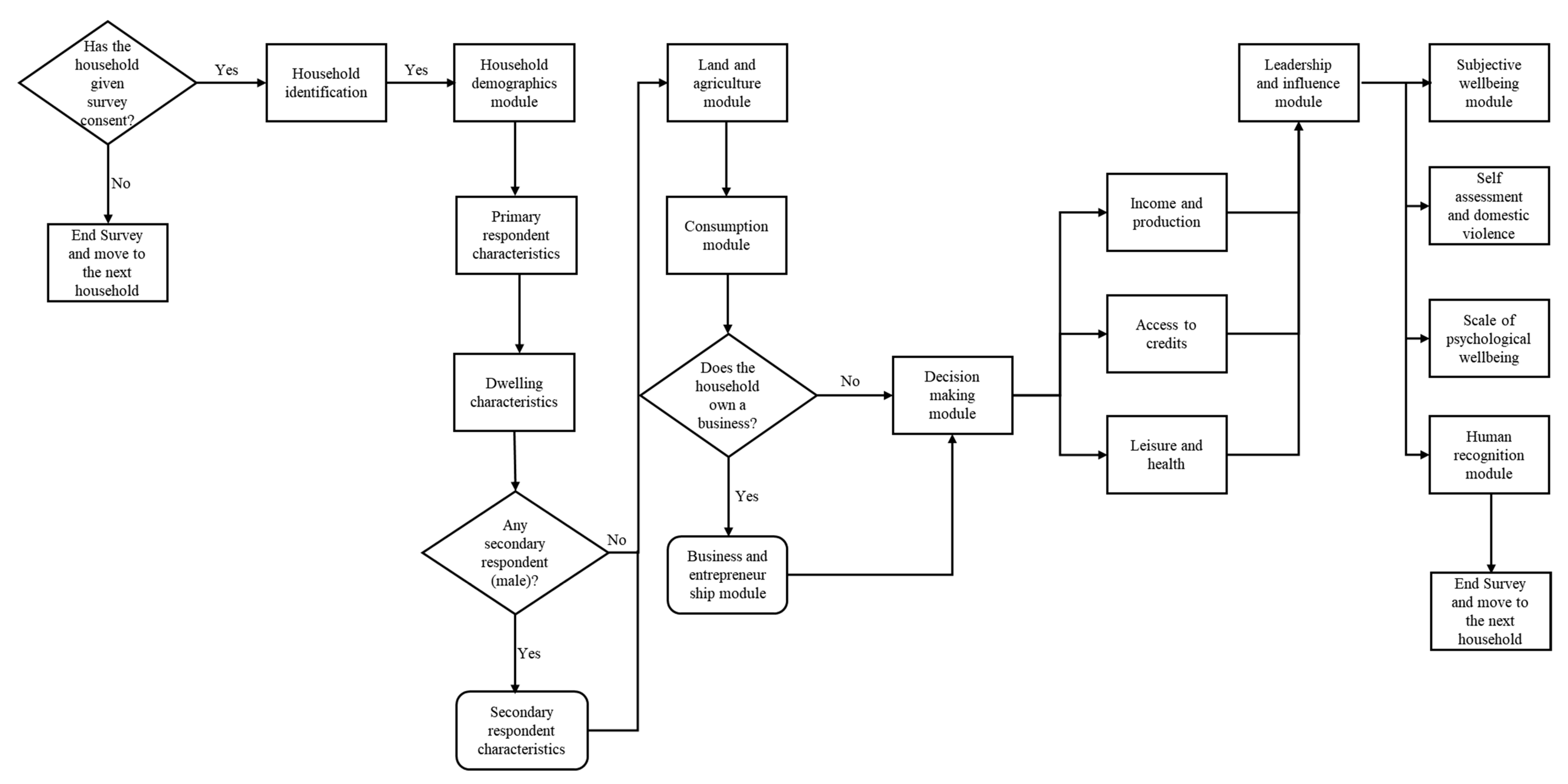
With this in mind, we start our investigation by isolating the indicators of violence, humiliation, dehumanization, and lack of autonomy, as the indicators of negative human recognition provision, within three domains namely, self, household and community. First, we extract indicators of negative human recognition from secondary data from Malawi Demographic and Health Surveys, herein referred to as Malawi DHS, for 2005, 2010 and 2015 [22] as shown in Table 1. We then include these indicators in the human recognition module prepared for the household questionnaire, as part of the study (see Figure 3).

Next, using data from Malawi DHS for the indicators outlined in Table 1, we, estimate the human recognition deprivation index (HRDI), headcount ratio, deprivation intensity and negative human recognition scores for women farmers [20,21]. We find that on average, 17% of women farmers in Malawi are human recognition deprived with deprivation intensities ranging up to 43%. Deprivation intensities also vary by human recognition domains and geographical location [20,21]. Thus, we establish the prevalence proportion (17%) of negative human recognition among women farmers in Malawi and take the next steps to design a suitable multilevel sampling approach to investigate this prevalence in our field data collection.

2.2. Study Area

Our field study took place in Malawi, a landlocked country in southeastern Africa located at latitude, 13.2543 south and longitude, 34.3015 east. Malawi shares its border with Zambia to the northwest, Tanzania to the northeast and Mozambique to the east, south and west. Malawi’s total land area is about 118,000 km² (45,560 square mile) with an estimated population of about 18 million people. Human development indicators show that about 72% of the Malawian population live below the poverty line [23]. Agriculture is very important in Malawi [24,25]. On average, 81% of the Malawian workforce employed in agriculture are women [23].

Since our target population are women farmers in Malawi, we outline the state of agriculture and land rights for women farmers in Malawi. Most Malawian farmers cultivate less than 1 hectare where they grow maize, beans, peas, and groundnuts as their main crops [25]. In Malawi, women farmers face constraints in land ownership and land use in the short and long-term. This is because a large share of Malawi’s land is held under customary law and kinship status is used to identify who has access rights to customary land [26]. Two main social systems in Malawi define how land rights are passed on: a patrilineal system, where land rights are passed from father to son, and a matrilineal system, where land rights are passed on through mothers to daughters. However, current land access rights for Malawian women farmers do not reflect an equitable distribution of land resources. On average, men hold 76% of land management rights compared to 23% for women. Only 17% of Malawian women have sole ownership of land, which is measured as a proportion of all household documented land [27]. These unequal rights in land and resource allocation are influenced by how women are viewed, valued and treated among themselves, their household and community (institutions) as well as their bargaining power in claiming productive resources for use.

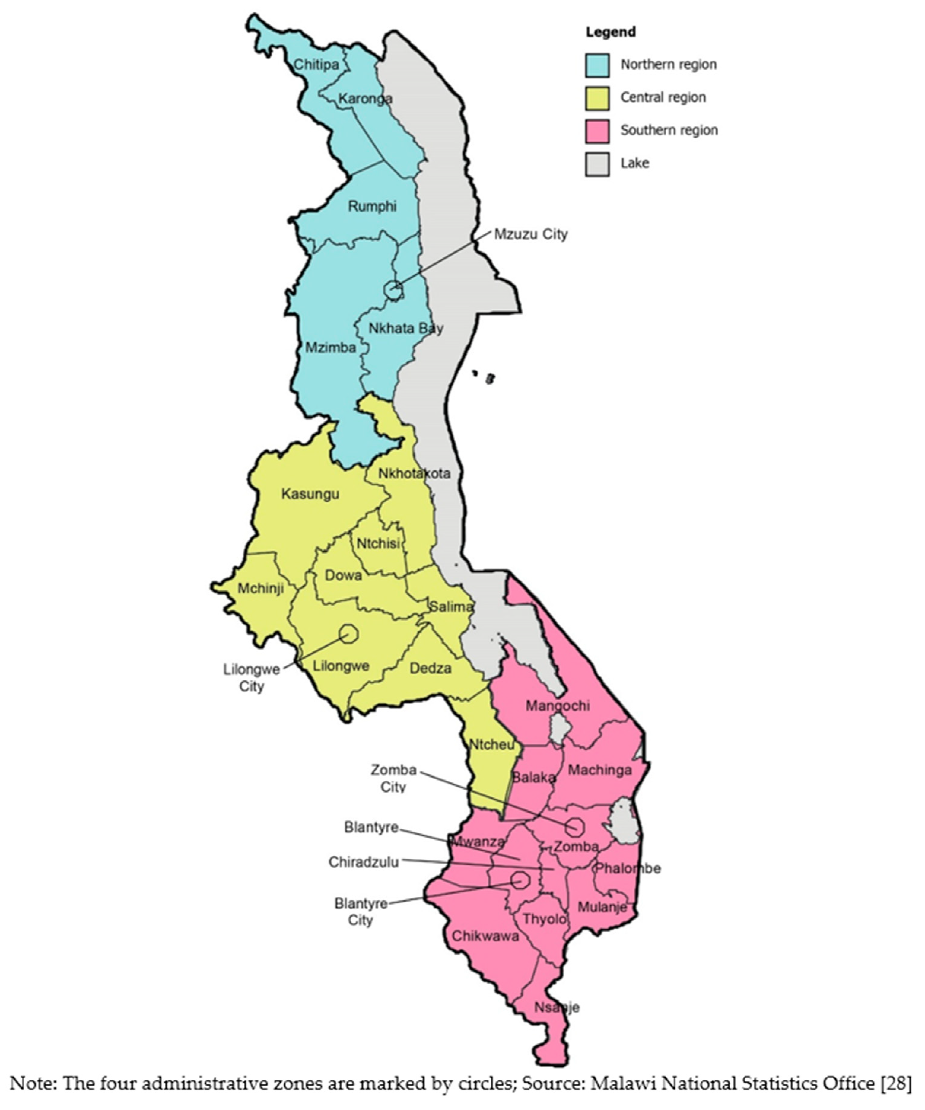
Going forward, we establish the administrative and geographical layout of Malawi to facilitate our survey sample mapping. Administratively, Malawi is divided into 28 main districts and four main government administrative zones. These districts and administrative zones are located within three regions namely north, central and southern regions as shown in Figure 1.

First, obtaining GIS information of Malawi’s districts, administrative zones and census data is important towards establishing district boundaries and determining the adequate sample size for our survey. Administrative level population or geographical data is vital to robust survey data. Geographical data like boundaries are used to select and set geo-fences of sampling units as well as map households to be sampled in the field, if spatial sampling is included in the survey design. Data granularity such as village-level census data or household listings are used to select sampling units, calculate required sample size and to increase the precision of survey estimates [29]. With this in mind, we obtain census data for the three geographical regions in Malawi from Malawi National Statistics Office [28].

Table 2. Malawi regions with 2008 population and 2017 projections.

Region	2008 Regional Population	% of Population	% of Population: Male	% of Population: Female	2017 Regional Projections
Northern Region	1,708,930	10%	6%	7%	1,360,195
Central Region	5,510,195	44%	21%	21%	6,046,725
Southern Region	5,858,035	46%	22%	23%	6,384,967
Total	13,077,160	100%	49%	51%	13,791,887

Source: Malawi National Statistics Office [28].

outlines the official 2008 census numbers with projections for 2017 for each region respectively. It also outlines the percentage distribution of the male and female population by region with regards to the overall population. As of 2008, 51% of the Malawian population were female while 44% of the overall Malawian female population lived in the central and southern region.

In Malawi, each region is divided into districts. These districts are further divided into varying numbers of traditional authorities (TA)s with populations ranging from 4 to over 200,000 people [28]. However, we could obtain population data down to the TA level only. We did not observe nationally collected population or geographical information beyond the TA level. Given this lack of information on the population size at the village level or geographical data on streets and/or household listings, it is important that we derive a different approach to survey sampling in this limited information context.

2.3. Random Spatial Sampling and Location of Starting Points Using ArcGIS 10

We select the main sample regions as the two most populous regions, namely: the central and southern regions of Malawi, because about 90% of the Malawian population live in these two regions. Using population proportional to estimated size (PPES) methodology, we select five districts covering both the central and southern regions of Malawi (see

Table 3. Sampled Malawi regions and districts with official 2008 population.

District	Region	2008 Population
Lilongwe rural	Central	1,230,834
Salima	Central	337,895
Chiradzulu	Southern	288,546
Mangochi	Southern	797,061
Nsanje	Southern	238,103

Source: Malawi National Statistics office [28].

). PPES is a sampling technique that uses a measure of size like population size or census data, if available, to determine a sampling unit’s probability of selection [29]. Since we had census data on population in the districts for 2008 and projections for 2017, we use PPES to select a fixed number of districts (5) within the selected regions (central and south).

The five sampled districts make up about 27% of the overall country population [28] (see United Nations [29] on the calculation of PPES). It is important to note that the aim of our study survey was not to provide a representative survey of the whole country but to estimate the prevalence of a human development component, which is human recognition, in a sub-sample of women farmers in Malawi. Going forward, we use ArcGIS 10 [30] to map the five selected district polygons on a base map. Using the sampling analysis tool for ArcGIS 10 [30], called fishnet grids, we superimpose a 25 × 25 km grid squares with centroids on the base map of the selected districts and a polygon of the TAs within each selected district (see Thomson et al. [31] and Galway et al. [32] on selecting primary sampling units (PSUs) from gridded population data). The TAs in the central and southern region range from 3 in Mwanza district to 15 in Lilongwe rural. This excludes Lilongwe city which has 58 TAs and Blantyre city which has 26 TAs.

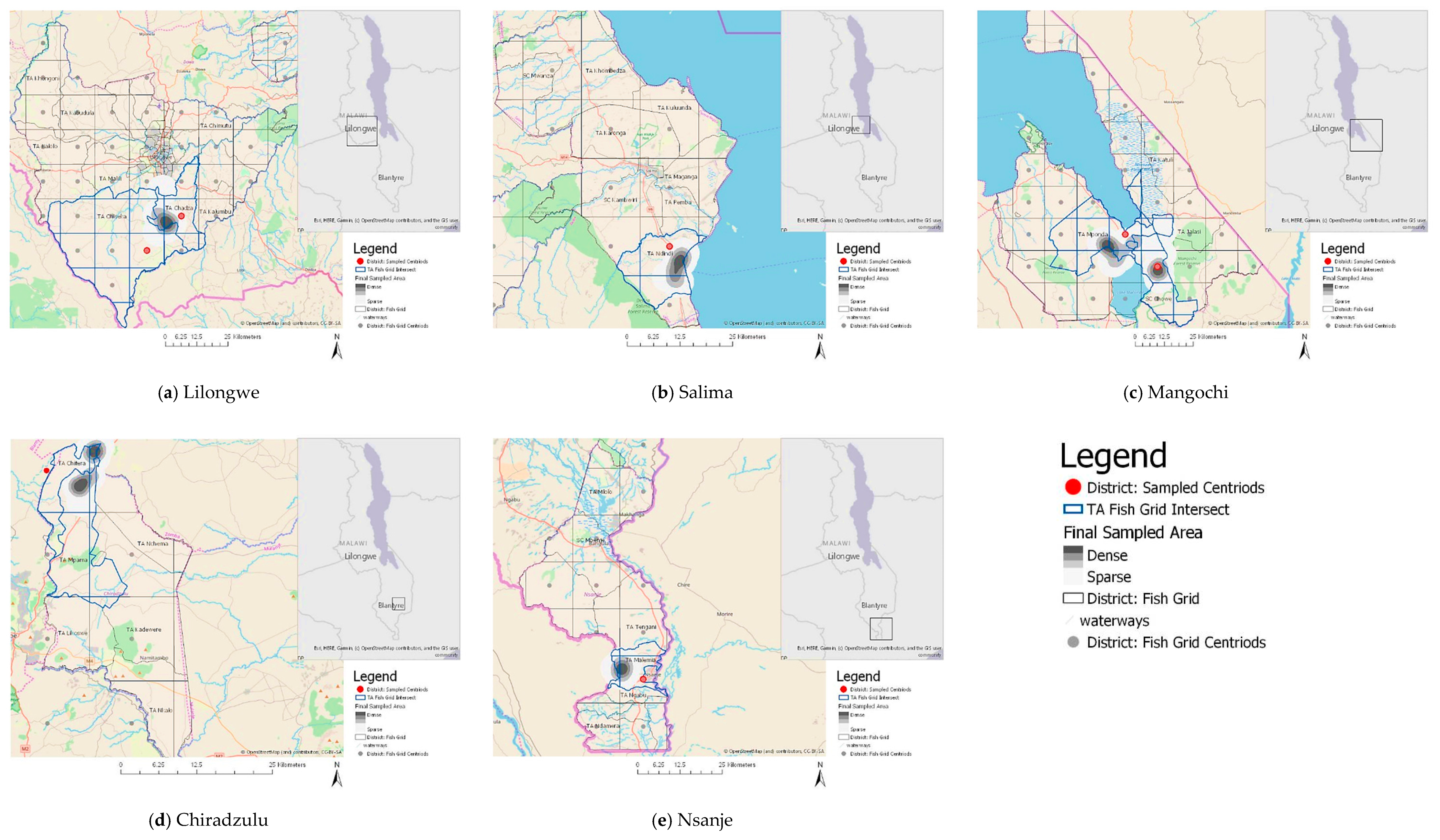
We randomly sample the grid centroids to select the starting points. We then select the nearest village areas to the sampled centroid as the base for the ground data collection (see Figure 2 and

Table 4. Sampled Malawi regions and districts with 2017 projection and village starting points.

District	Region	2017 District Projections	Starting Points
Lilongwe rural	Central	1,161,408	Mitundu
Salima	Central	445,031	Chipoka
Chiradzulu	Southern	327,038	Namadzi
Mangochi	Southern	1,091,666	Mangochi rural
Nsanje	Southern	295,900	Chididi
Total		1,693,732

Source: Malawi national Statistics Office [28].

). It is also important to note that the starting points only indicate the general area where the survey should start from. It neither constrains the number of households interviewed nor sets a village limit boundary for these areas.

Given our study focus on women farmers, the highly developed urban TAs in Lilongwe district were excluded from the sampling tool. Finally, we established the TAs to which these starting points belong to and established their estimated population projection for 2017 as shown in

Table 5. Population projection in TAs with the sampled starting points.

District	Region	2017 District Projection	TA	TA Population: % District	2017 TA Projection	Starting Points
Lilongwe rural	Central	1,161,408	Chadza	9%	105,900	Mitundu
Salima	Central	445,031	Ndindi	12%	53,012	Chipoka
Chiradzulu	Southern	327,038	Chitera	6%	20,848	Namadzi
Mangochi	Southern	1,091,666	Mponda, Chowe	28%	298,161	Mangochi rural
Nsanje	Southern	295,900	Malemia	5%	14,175	Chididi
Total		1,693,732			250,968

Source: Malawi National Statistics Office [28].

.

3. Fieldwork: Survey Preparation

3.1. Sample Size

Our primary research objective was to sample women farmers, collecting information on the indicators of human recognition as well as socio-economic and social demographic characteristics under budget constraints. Particularly, we wish to establish that negative/positive human recognition exists in a sub-sample of women farmers in Malawi as observed in the secondary data (Malawi DHS). However, one challenge to our study objective, as noted by United Nations [29] is arriving at the right combination of cost savings and precision loss associated with multilevel sampling design such as ours. We note that in cluster sampling, correlation among sampling units may inflate the sample variance and reduce the precision of the survey estimates compared to non-clustered units. As a result, survey sample size must consider the design effect of the sampling method especially for multilevel sampling design. Design effects measure the factor by which an estimate variance obtained from a simple random sample must be multiplied to account for the actual survey design complexity due to clustering, weighting and stratification [29,33,34]. That is, design effects measure the increase in sample size needed to get the same power as a simple random sample. The design effect for an estimate like, for example, the mean, can be shown as:

$$D(m)=1+(b-1)\rho$$

(1)

where $D(m)$ is the design effect of an estimated mean, $(m)$; $\rho$ is the intraclass correlation; and $b$ is the average cluster sample size. Studies have shown that most design effects range between 2 and 4 and depending on the measure of interest, can be higher as well [33,34,35]. Design effects are usually calculated from existing studies of the target population if the target data are representative and if there is some pre-existing knowledge of the study population [33,34]. Once the design effect is estimated, the sample size needed to estimate a specific prevalence proportion of a particular phenomenon in a target population can be shown as:

$$n=D\ast \frac{{\mu }_p(1-{\mu }_p)}{se{(p)}^2}$$

(2)

where $D$ is the design effect, $n$ is the sample size, ${\mu }_p$ is the prevalence proportion we wish to estimate, and $se(p)$ is the acceptable standard error (SE) of $p$. Finally, one can calculate the adjusted sample size, corrected for an estimated finite population, $n_{adj}$, as follows:

$$n_{adj}=\frac{n}{1+\left(\frac{n-1}{N}\right)}$$

(3)

where $n$ is the sample size, estimated from Equation (2), and $N$ is the estimated population size in the target sample area.

We estimate the design effect from the Malawi DHS for women farmers using the mean negative human recognition scores. DHS data are gotten from two-staged probability sample designs derived from existing sample frames like census data [36]. DHS sample design uses areas that are homogenous e.g. regions and urban/rural areas, as strata. In the first stage, primary sampling units are selected by population proportional to size (PPS) method within each stratum. In the second stage, a fixed number of households are selected by probability systematic sampling from the complete listing of households in the selected clusters [36]. The generated probability systematic sampling values are then used to calculate the sampling weights for each primary sampling unit (PSU), household or individual.

We normalize the individual weight for women respondents present in the Malawi DHS datasets by dividing the probability variable with 1,000,000 (one million) as recommended by the DHS manual [36]. We then set the complex survey design parameters by applying the primary sampling unit or cluster variable, the stratification variable, and the normalized weight variable using svy command in STATA [37]. Finally, we calculate the negative human recognition scores from Malawi DHS using indicators in Table 1 above, re-scaling and allowing our final values to lie between 0 (lowest negative human recognition) and 100 (highest negative human recognition score). Then, we calculate the design effects of mean negative human recognition values from the Malawi DHS using the design and misspecification effect function in STATA.

Table 6. Estimated design effects for women in Malawi by year and occupation: Mean negative human recognition.

	Negative Human Recognition	Mean	SE	DEFF	DEFT	MEFF	MEFT
2005	Non-Farmer	29.46	0.26	2.12	1.46	2.05	1.43
2005	Farmer	31.04	0.34	2.61	1.62	2.73	1.65
2010	Non-Farmer	29.72	0.28	1.86	1.36	1.74	1.32
2010	Farmer	30.11	0.29	1.76	1.33	1.91	1.38
2015	Non-Farmer	31.10	0.27	1.65	1.28	1.62	1.27
2015	Farmer	31.81	0.26	1.37	1.17	1.38	1.17
	Observations	19,282

Source: Malawi DHS; Note: SE= Standard error.

presents the design and misspecification effects, DEFF & DEFT and MEFF & MEFT from the Malawi DHS for women, by year and by occupation as farmer or non-farmer. It shows that on average, women farmers have higher negative human recognition than their counterparts in Malawi. It also shows that the design effects (DEFF) and misspecification effects (MEFF) needed to calculate mean negative human recognition for women farmers range from 1.4 to 2.6, and from 1.3 to 2.7 respectively.

Going forward, we isolate the design effect by the five selected districts slated for the primary survey from the Malawi DHS as shown in

Table 7. Estimated design effects for women farmers only by the five selected districts in Malawi: Mean negative human recognition.

Year	District	Mean	SE	DEFF	DEFT	MEFF	MEFT
2005	Chiradzulu	25.24	11.56	1.02	1.01	0.85	0.92
	Lilongwe	30.07	1.22	2.85	1.69	1.69	1.30
	Mangochi	28.45	0.97	1.03	1.01	1.78	1.34
	Nsanje	31.71	1.42	1.45	1.20	1.23	1.11
	Salima	31.09	0.87	0.41	0.64	1.28	1.13
2010	Chiradzulu	28.19	0.74	0.85	0.92	1.80	1.34
	Lilongwe	28.94	1.15	2.29	1.51	1.27	1.13
	Mangochi	24.11	1.48	1.38	1.18	1.11	1.05
	Nsanje	30.57	1.16	0.67	0.82	2.08	1.44
	Salima	29.58	1.06	0.48	0.69	0.78	0.88
2016	Chiradzulu	30.81	1.24	0.72	0.85	1.37	1.17
	Lilongwe	34.58	1.15	2.19	1.48	0.78	0.88
	Mangochi	28.61	1.01	0.90	0.95	0.75	0.87
	Nsanje	28.39	1.29	0.28	0.53	0.65	0.80
	Salima	29.03	1.38	0.70	0.84	1.09	1.04
	Observations	3987

Source: Malawi DHS; Note: SE = Standard error.

.

The average design effect for mean negative human recognition for women farmers in Malawi is approximately 2. According to Salganik [33], once the design effect is established from existing representative literature and/or data, one can calculate the required sample size with regards to a desired standard error. As initially noted, about 17% of the women farmers in Malawi are human recognition deprived, and thus, we estimate the sample size needed to examine 17% prevalence of negative human recognition for women farmers with a standard error no greater than 3.4%, a 95% confidence interval (z-score = 1.96) and a design effect of 2. Using Equation (1), we calculated the desired sample size, $n$, as follows:

$$n=2\ast \left(\frac{(0.17)(1-0.17)}{{(0.034)}^2}\times {(1.96)}^2\right)\simeq 937$$

(4)

Thus, we need a total sample of 937 women farmer respondents for our study. Adjusting for finite population using Equation (2) and plugging in the population totals calculated in Table 4 at the district level and TA level, we estimate the final adjusted sample size at the district and TA levels as follows:

$$\begin{array}{l}n{(District)}_{adj}=\frac{937}{1+\left(\frac{937-1}{1,693,732}\right)}\simeq 937\\ \\ n{(TA)}_{adj}=\frac{937}{1+\left(\frac{937-1}{250,968}\right)}\simeq 934\end{array}$$

(5)

Thus, in line with Salganik [33], Grais et al. [16], Fearon et al. [34] and Wejnert et al. [35], we set our desired maximum SE to 3.4% (0.034) within a 95% confidence interval (CI), correcting for finite population. This provides us with a final total sample size between 934–937 respondents (an average of 187 women farmers by TA in each district or by district alone).

3.2. Field Hardware and Software

We developed and prepared the household questionnaire modules (see Figure 3) for the field data collection using survey software from Dooblo Limited [38]. The questionnaire contains seven modules including a human recognition and subjective wellbeing module. We purchased a survey package of 1000 interviews to facilitate our data collection and programmed the household questionnaire modules using the survey software.

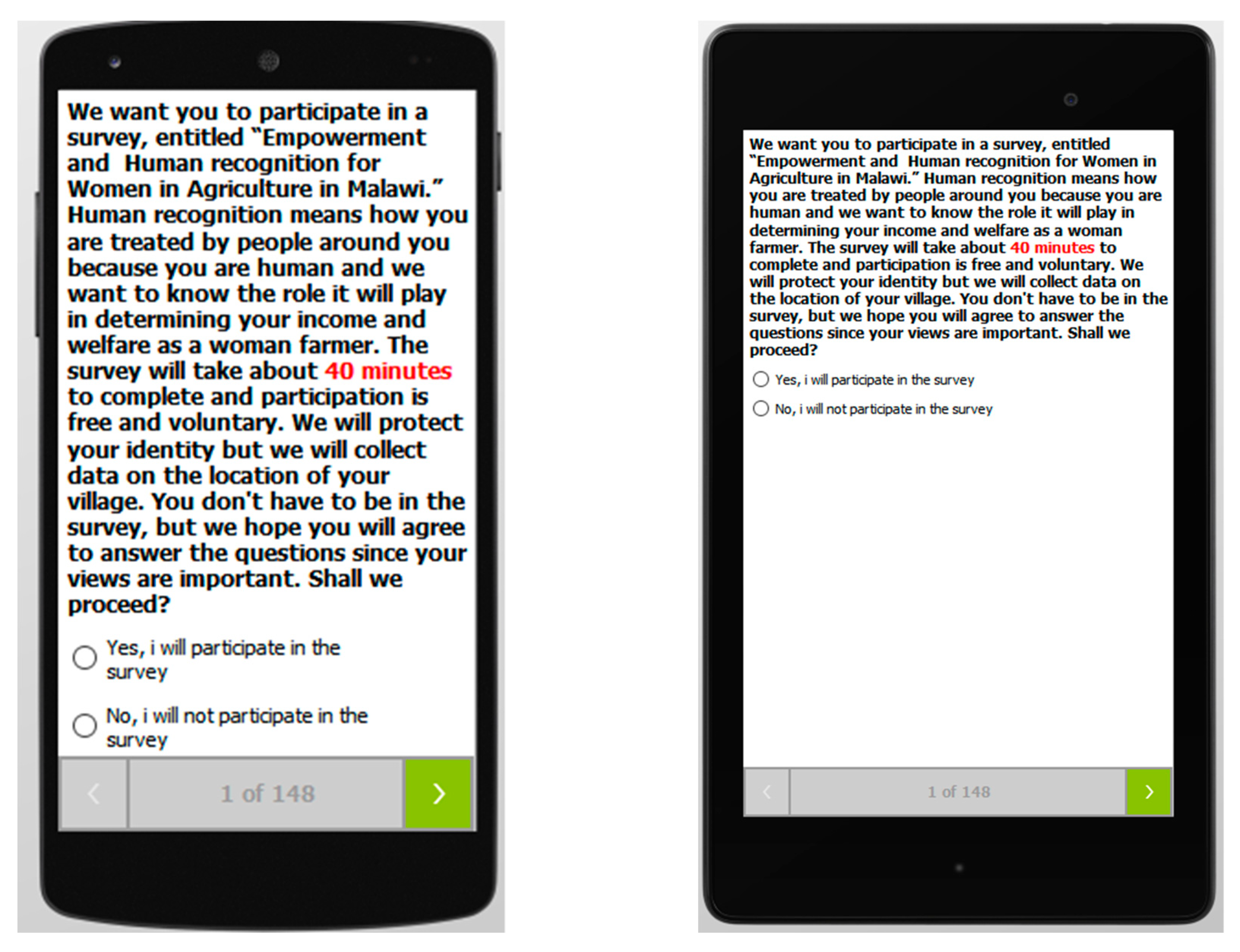
The questionnaires were transferred to four handheld Android 4.2-based PDAs using the survey software application services. Each PDA was equipped with a standard mobile SIM to support internet connectivity and real-time cloud upload of survey data. Data transfer was facilitated from the PDA to the computer via cloud upload, and from computer to PDA via synchronization of survey software. The main data capture software consists of a (1) desktop designer application for designing the survey questionnaire, (2) a cloud database for storing the finished questionnaire and collected data in various formats including Microsoft excel, and (3) a mobile application (android- and windows-based) which transfers the finished questionnaires from the cloud database to the PDA and finished data from the PDA to the cloud storage. The PDAs also stored the completed questionnaires on the device memory in the absence of internet connectivity. The data capture software allows the incorporation of logical statements into the questionnaires which were then validated at the point of data entry. Customized error messages, question skipping, password-protection of the questionnaire, and geo-fencing were options available in the software. The software also supported multiple user accounts with unique identifying numbers allowing individual records from field interviewers to be tracked for quality purposes. Overall, the finished field questionnaire was designed to accommodate a range of entries including drop downs, radio selections with single or multiple buttons, and text field entries. They were tested on different screen displays before the commencement of the field survey (see Figure A1). Other hardware such as four 500 mAh mini power banks were purchased in addition to two 20000 mAh power banks to account for the unpredictable nature of electric supply within the country. The four 500mAh were assigned to a specific PDA, labelled 1–4 to ensure accountability in case of technical malfunctions.

3.3. Training

Female field interviewers were recruited and trained in a 5-day training session to familiarize them with the PDA, GIS/GPS technology and survey content. The recruited female field interviewers were informed on the sensitive nature of the human recognition module with regards to women farmers, and at the time of recruitment, were required to have completed their bachelor’s degrees. Specifically, the field interviewers were given the programmed PDAs to practice with, enabling them to gain familiarity with the questions. During the training, emphasis was placed on confidentiality, anonymity and privacy of the female respondents. All necessary protocols needed for an ethical research were presented to the field interviewers to guide them in the data collection. As the field interviewers were required to translate the questions from English to the native language prevalent in Malawi (Chichewa), we ensured that each selected field interviewer was fluent in English and at least two native languages in Malawi including the Yao, Sena, Ngoni, and others. To reduce measurement error that could arise from translating the questionnaire from English to Chichewa, we discussed each question during the training session and field interviewers established consistent wordings that best communicated the questions, to be used in the field interview. The questions in the questionnaire were also simplified accordingly for ease of interpretation and translation. Finally, the field interviewers were given additional training in PDA maintenance, battery charging, troubleshooting, and data backup.

3.4. Systematic Random Sampling of Households

The field work for the study was conducted between May and July 2017. Field interviewers used the village center in the starting points as anchor points to form an outward-facing wide circle with the interviewers facing north, east, west and southward from the village centers. This cardinal configuration was swapped for starting points only (five times in total), in anticlockwise rotation i.e., north-facing field interviewer was required to move west, and south-facing field interviewer was required to move to the east etc. In the case of null results from village centers in the starting points like if the village mapped as the starting point was an empty field, the nearest village from the mapped starting point is used as the new starting point for the survey. From the selected village centers, the field interviewer used systemic random sampling with random walk protocol to select the households within the villages. Random walk is a household selection technique that enables face-to-face interviews in areas with no population register, with the assumption that it creates equal sampling probabilities of households [39]. Random walk protocol involves protocol for household selection, which is counting from the first house on the left side of the street to select the household to be interviewed from the random selection key numbers, spreading/fanning out over the village inhabitants, and protocols for non-residential or empty household selections. For instance, if the field interviewer found the next random household to be non-residential, an empty household or a vacant lot, the field interviewer is required to survey the next residence opposite the initially selected residence, to its right, and so on.

Random selection key numbers using Microsoft excel RAND function were generated and used by field interviewers in selecting interviewed households (Excel RAND function returns an evenly distributed random real number greater than or equal to 0 and less than 1. Number ranges can also be set to start from 1 to any maximum e.g. 1–5 or 1–100. A new random real number is returned every time the worksheet is calculated. As of Excel 2010, Excel uses the Mersenne Twister algorithm (MT19937) to generate random numbers for the RAND function.). The RAND skip interval was set between 1 and 5 as the field interviewers reported on the first day that bigger numbers resulted in skipping most of the houses in the villages because of the irregular layout of some villages. When an eligible household with an inhabitant is encountered, the field interviewer enquires about the head of the household. Once the household head is established, the field interviewer interviews the head of the household if female or the female spouse/partner, if head of the household is male. 80% of Malawians live in rural areas and depend on agriculture for their livelihood. Consequently, most women respondents we encountered during the survey were mostly farmers.

3.5. Field Team and Logistics

The survey team consisted of one survey vehicle with one team supervisor and the rest of the field interviewers armed with programmed PDAs, information on starting points, random number keys for systematic household selection, and the random walk protocol. Each field interviewer was assigned a PDA number, a user ID and password to facilitate PDA login. A typical data collection day started at 7 am in the morning and ended at 4 pm in the evening and each field interviewer was required to interview about 14–15 respondents every day. Each field interviewer was also required to continue from where they had stopped the household selection from the previous day. As a result, the number of required respondents in the sample district took about 3.5 days to complete. The field interviewers were then moved to the next district to start another round of data collection.

The team supervisor always met with the head of the TAs in the selected survey area the day before to inform them about the study. The interaction with the head of the TAs helps to decrease any suspicion against the field interviewers and made the respondents more receptive to the questions. Eligible households were defined as those having a woman farmer as part of the household leadership structure, either in a dual-headed or single-headed household. Each eligible household can only be selected once in the course of the survey. As most of the approached households were willing to participate in the survey, only a small number of households were replaced by additional household selection. At the end of the survey, all collected data including GPS information were synchronized with the cloud database. Key performance indicators were also synchronized and analyzed. Field interviewer performance indicators like speed of survey completion and quality of answers were monitored using the in-built monitoring system in the survey software.

4. Field Results

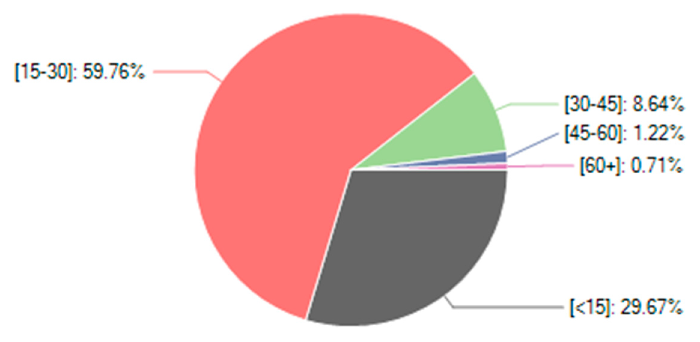
As the end of our field survey, we collected data from two districts in the central region namely: Lilongwe (7 villages), Salima (7 villages); and three districts in the southern region of Malawi: Mangochi (8 villages), Chiradzulu (7 villages) and Nsanje (10 villages). As our method uses village starting points for the survey, the field interviewers were able to fan out across several villages within each TA, in the course of the data collection. Our collected data yielded 933 respondents and about 1% data loss, given our maximum estimated sample size of 937. Our household questionnaire sampled female-only and dual-adult households (those with male and female adults) with women farmers as the main respondents. Each field interviewer interviewed the required number of respondents i.e., about 14–15 respondents per day. Over half of the interviews where completed between 15–30 min as shown in Figure 4.

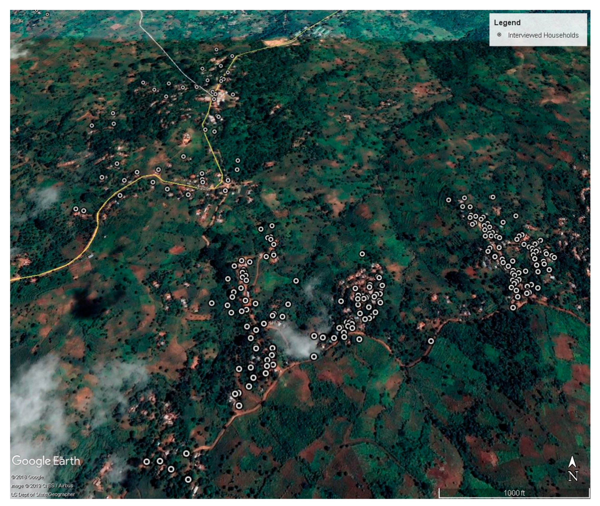
Finished interview GPS coordinates were processed and mapped using ArcGIS 10 [30] on the initial sample grid selections with distance displacements. Figure 5 shows the distribution of the sampled respondent data within the selected grid, while Figure 6 shows an excerpt from some of the sampled villages in Nsanje district.

Field Interviewer Performance Indicators

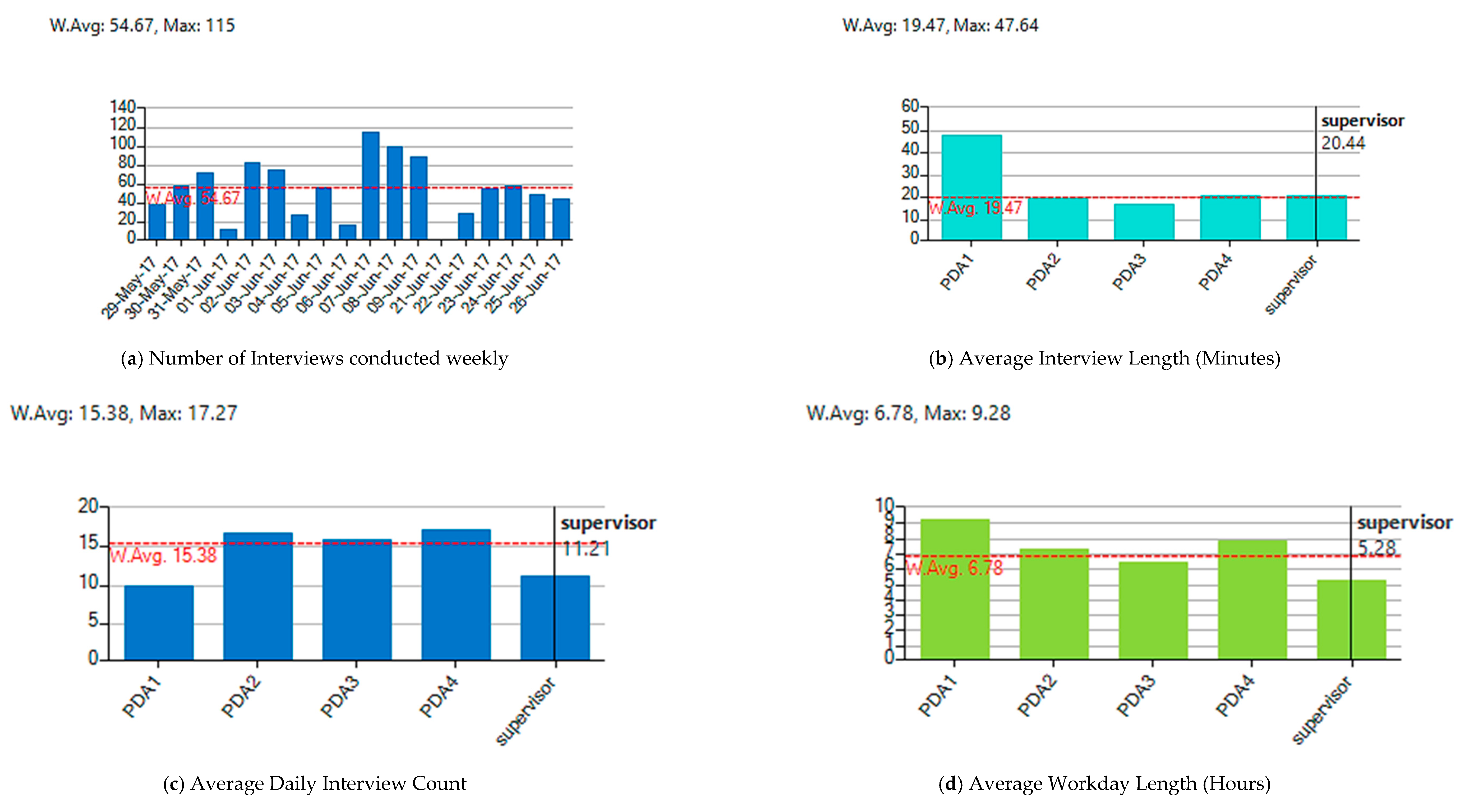
After the survey, the data were downloaded and analyzed using Microsoft excel, ArcGIS 10 and STATA 14. Field interviewer data were also analyzed using software in-built performance indicators. Overall, a total of 18 days were spent in active field work (including travel dates from one location to another) with an average of 54 interviews conducted weekly from the field interviewers. We maintained an average workday length of 6 h, including an hour of breaktime in between and all field interviewers collected 100% GPS information from the location of interviewed households (See Figure 7).

5. Post Survey

Data Validation Using Malawi DHS

The success of a sample design can be checked by evaluating how comparable estimated parameters like the mean and median are with values extracted from the nationally represented datasets [9]. In other words, how similar are the mean or median values observed in the survey data, when compared to the values observed in the nationally representative data. Thus, we evaluate the performance of our survey design by comparing the mean and median negative human recognition score for sampled women farmers with that calculated from Malawi DHS for 2004, 2010 and 2015 [22] (see [20,21] for the definition, indicators and calculation of human recognition scores in general and for women in Malawi). The Malawi DHS dataset contains information on the demographic and socioeconomic status of randomly sampled respondents (women) aged 15–49. Using indicators from the Conflict Tactics Scale (CTS) and domestic violence module (see Table 1, above for outline of indicators used in both surveys), we calculate the mean and median negative human recognition score for women farmers for both the Malawi DHS and our collected primary data (Note that the questions from the Conflict Tactics Scale (CTS) and domestic violence module in both the Malawi DHS datasets and the primary survey are the same, except for some word consolidation). We set the multilevel complex survey design parameters for our primary data by applying the primary sampling unit variable (district), the normalized weight variable and the finite population value at the district level using the svy command in STATA.

Table 8. Mean negative human recognition score of sampled women farmers from primary survey.

	Mean	Standard Error (SE)	95% CI
Negative human recognition	26.76	0.63	25.02–28.50
Observations	933
Population size	1,693,732
PSU	5
Design DF	4

Source: Authors calculations from primary data; Note: SE = Standard error.

shows the mean human recognition score calculated for sampled women farmers from our primary survey. Women farmers from these selected areas have on average a human recognition deprivation score of 26, which is 2.53 points lower than the pooled average from Malawi DHS for the five selected districts.

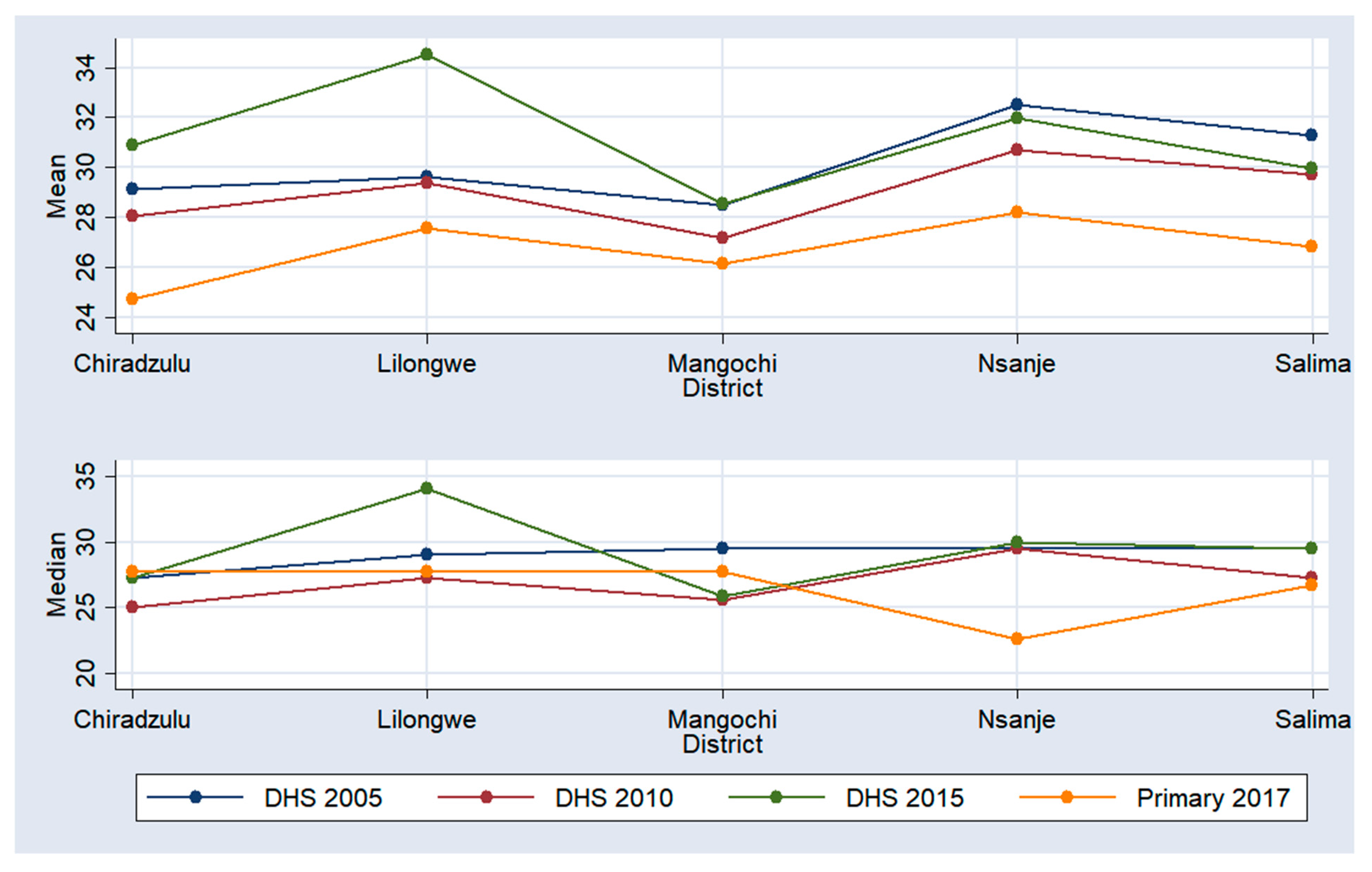
We further compare the mean and median distribution of negative human recognition for the five selected districts with that from the Malawi DHS. Figure 8 shows the mean and median human recognition score for sampled women farmers from our survey and from Malawi DHS for 2004, 2010 and 2015.

The yellow line shows the district values from our 2017 survey data while the other lines show the district values from Malawi DHS. The mean and median negative human recognition scores from the 2017 survey dataset fall within a comparable range when examined together with the Malawi DHS for women farmers. Finally, we compare how much the averaged negative human recognition observed in the primary data changed, relative to the pooled average from the Malawi DHS at the district level.

Table 9. Mean negative human recognition and unit difference from pooled district average of Malawi DHS: women farmers only.

District	Mean (2017)	Mean (Pooled DHS Data, 2005–2015)	Unit Difference
Chiradzulu	24.71	28.08	−3.38
Lilongwe	27.58	31.20	−3.62
Mangochi	26.13	27.06	−0.93
Nsanje	28.21	30.22	−2.01
Salima	26.83	29.90	−3.07
Observations	933	19,282
Population size (District)	1,693,732	19,377
PSU	5	2185
Design DF	4	2130

Source: Malawi DHS [22], Author’s calculations; Notes: Unit difference = Mean (2017)—Mean (Pooled data, 2005–2015).

shows the mean negative human recognition and the unit difference from the pooled district average of Malawi DHS for women farmers only.

The mean negative human recognition score ranges from 24 (Chiradzulu) to 28 (Nsanje) and 27 (Mangochi) to 31 (Lilongwe) in the primary and Malawi DHS respectively. We also compare the unit difference across the different districts in the study and show that, compared with the nationally representative average, unit difference ranges from −0.93 to −3.62 (Note that further analysis of the empirical data derived from this field survey are beyond the scope of this article.).

6. Discussion and Limitations of the Sampling Approach

As we derive learned lessons from quantitative and qualitative analysis of our survey data, other limitations to our survey design and approach remain. For example, Kondo et al. [3] note that the availability of enough satellite imagery is one of the main challenges facing random spatial sampling for development research. Outdated satellite imagery and map layers often hinder proper spatial mapping and cause field confusion when mapped areas and field locations do not correspond.

Another challenge is that in using a grid method, one runs the risk of selecting only households in high or low density areas [16]. According to Grais et al. [16], ideally, a sample grid should be weighed by population. However, the authors found that this method can be costly and time consuming especially if population data is not available. Thus, a grid imposed on an area with both high- and low-density populations has a higher chance of capturing 50% of the population as the true representation of that population overall. As Malawi is a predominately rural with 80% of the population living in rural areas [23,40], and taking quantity and spread of farm lands into account, we argue that the population for women farmers is more uniformly distributed. In addition, our study aim is to collect the sample size required to estimate a fix prevalence value of negative human recognition for women farmers in selected Malawian districts only. As the survey data is not representative of the whole country, we argue that it is not necessary to weigh our sample grids by grid population. Nevertheless, we implemented the survey sample weights, calculated using the finite district population estimates for the survey year.

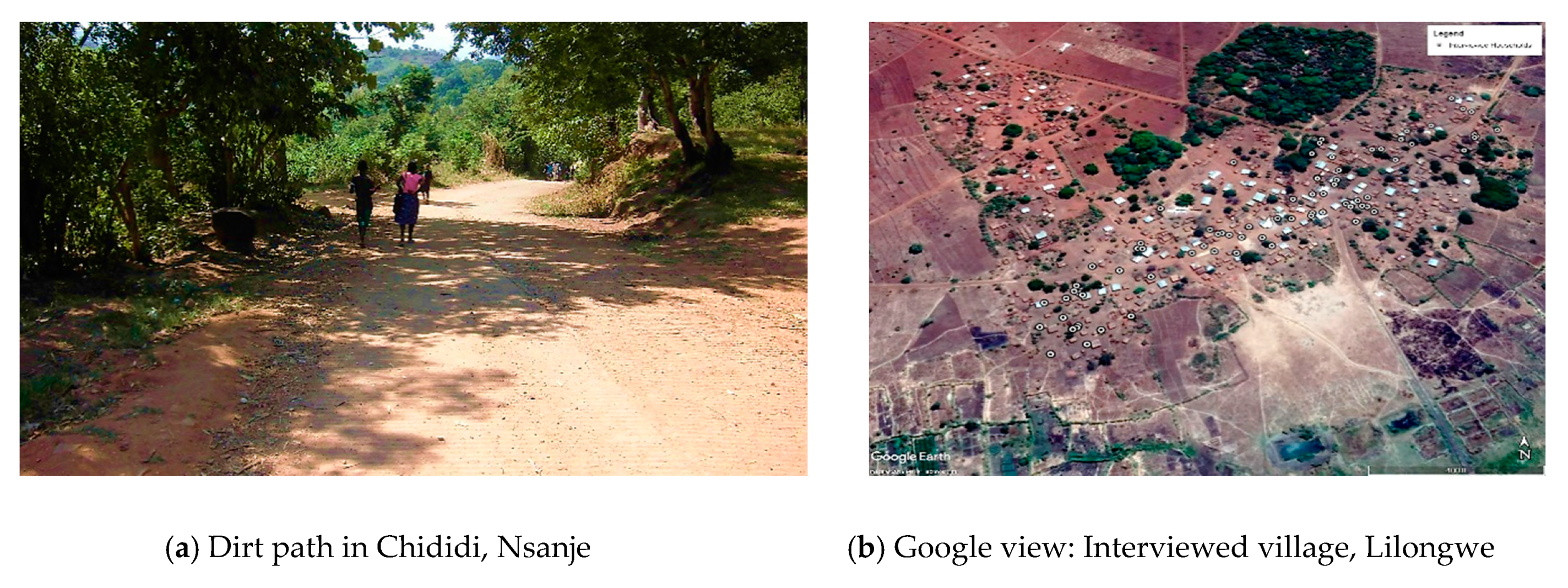
Random spatial sampling could potentially reduce sampling bias in surveys, however, field interviewers could introduce bias at the household sampling level through field interviewer discretion. As field interviewers are expected to select another household for the survey if the originally targeted household resulted in a null value, the household selection process and thus, field interviewer bias, will most likely vary by study types and by environmental factors. In our study, the combination of various bias mitigating methods from Kondo et al. [3], Shannon et al. [10] and Grais et al. [16] helped mostly reduce field interviewer discretion bias. Field interviewers reported that using village starting points made it easier to pinpoint where to start the household interviews. However, as most residential houses were not symmetrically aligned, village starting points also made it slightly harder to administer the systematic random sampling with random walk. Random walk protocols in household selection create the assumption of equal sampling probabilities of households in the survey vicinity [39]. However, Bauer [39], Eckman and Koch [41] and Himelein et al. [42] argue that random walk can lead to deviations in uniformity which create biases in the survey data. As shown with the random walk routes tested by Bauer [39], the deviations from the equal selection probability occur due to the basic routing specifications and the pattern of street network, increasing the possibility of certain houses being sampled more than others. Consequently, sample bias occurs if there are weak correlations between variable distributions and unequal selection probabilities. One way of reducing sample bias is providing field interviewers with plotted maps of the interview route to enable researchers to have control of the complete route and reduce selection bias early on [39]. Although we used random walk methodology in our study, we also highlight that our study focuses on rural villages in the selected districts in Malawi, where little or no street networks exist. Most households are on dirt paths, and most villages rarely contain long main streets (see Figure 9).

As a result, the field interviewers were not required to align the length of their random walk routes with the length of the streets as criticized in Bauer [39]. Field interviewer routes winded through from one village to the next as no village or city limit rules were included in the route instructions. Secondly, in our RAND skip list, we generated one random number per household to be interviewed. That means that when the field interviewer selects, for example, the number 2 as the random household number to be interviewed, the next household is selected by following the random walk protocol and counting, using the next new random number on the RAND list. Finally, we check for post-survey bias as suggested by Bauer [39], by examining the correlations between our variable of interest—negative human recognition—and the selection route proxied by the longitude and latitude values (GPS coordinates of the respondents) collected during the survey.

Table 10. Pairwise correlation coefficients for negative human recognition, longitude, and latitude of survey data respondents.

	Negative Human Recognition	Latitude	Longitude
Negative human recognition	1.00
Latitude	−0.02	1.00
	{0.59}
Longitude	−0.02	−0.60 **	1.00
	{0.49}	{0.00}

Source: Primary data; Notes: ** = Significant at 5% and below; p-values in curly {} parenthesis.

shows the pairwise correlation coefficients between the negative human recognition, longitude, and latitude values. We observe that negative human recognition is not significantly correlated with any of the GPS coordinates of the respondents.

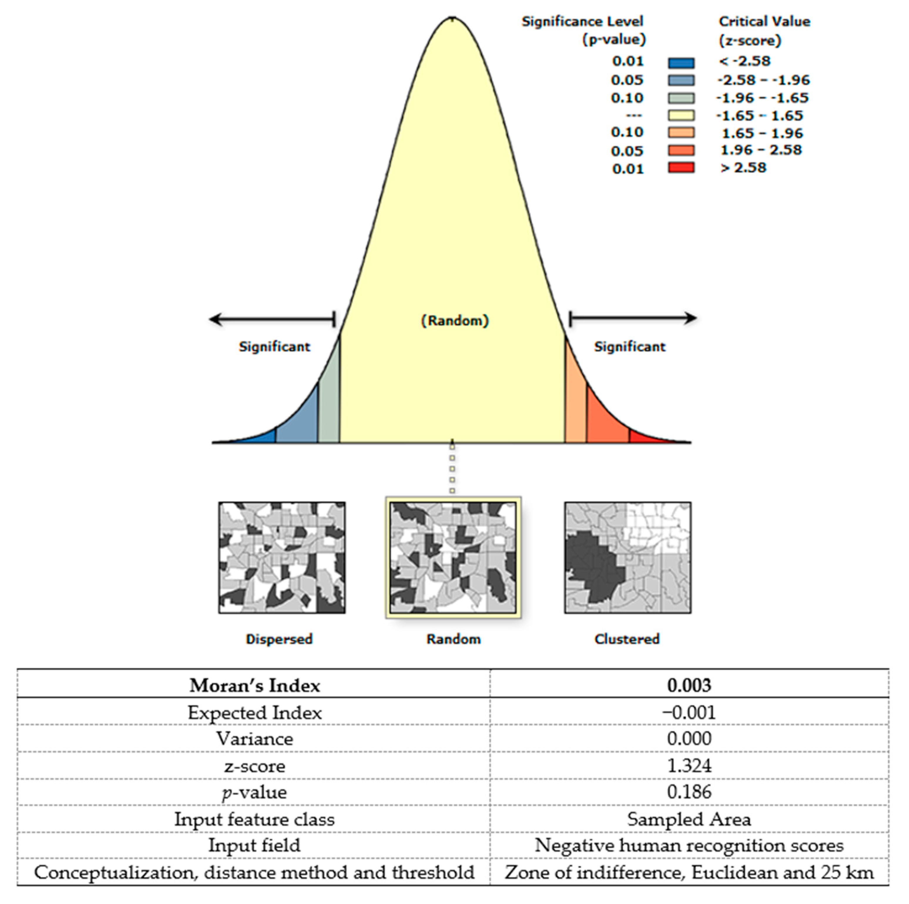
We further investigate the presence of spatial autocorrelation in our survey data. Spatial autocorrelation measures the presence of systemic spatial variation in the spatial distribution of that variable of interest. The presence of spatial autocorrelation introduces information redundancy into the survey data if sampled points are very close together and inflates the sampling variance of the estimate, for example, the sample mean. Haining [43] and Scott [44] argue that in multilevel survey designs, spatial autocorrelation can be solved by using systematic sampling with random starting points as we implemented in our survey design. In other words, incorporating the systematic sampling method should produce estimates with lower sampling variance. With this in mind, we implement the Moran’s Index statistic for measuring spatial autocorrelation in ArcGIS 10 [30]. The Moran Index (Moran I) measures the statistical likelihood that the observed data is randomly spatially distributed. Particularly, the null hypothesis is that the variable of interest being analyzed is randomly distributed among the features in the area of survey i.e., the spatial process involved in the pattern of values coming from our variable of interest is random chance. We set the spatial conceptualization as a zone of indifference and the distance method to Euclidean. Setting the spatial conceptualization to zone of indifference means that features within the specified critical distance (threshold distance) of the target feature will receive a weight of one and influence the computations for that feature. Once the critical distance is exceeded, the weights and the influence a neighboring feature has on target feature computations will diminish with distance (See the documentation on ArcGIS [30] for detailed information on spatial conceptualizations). We also apply the row standardization and set the distance threshold to 25 km, as is with the grid squares (see method section). Figure 10 shows the global Moran Index for negative human recognition in our primary survey data with accompanying correlation statistics.

Non-significant p-value and near zero Moran I statistics indicate that the observed spatial pattern of negative human recognition in the survey data exhibits compete spatial randomness.

However, it does not mean that there are no errors in the survey data. Errors like respondent bias may exist. United Nations [29] argues that such errors in survey data can occur through the questionnaire design, the dat a collection method and from the actions of the respondents. Ambiguity in problem question specification, wording, open and closed question formats, order of questions, and response categories are some of the problems which may introduce bias in the sample data. During face-to-face interviewing, respondent bias can be introduced through behavior traits like social desirability. In other words, if the respondent perceives certain events to be socially good or bad, the respondent may decide to under- or over-report the occurrence of that bad or good event, respectively [29]. Another source is the presence of other household members at the interview. In general, these measurement errors can be minimized through field interviewer training, supervision, and workload reduction. As our study focuses on eligible women farmers only, the field interviewers were required to interview the women alone and away from prying eyes. In most cases, the woman was taken to the section of the house or outside where she felt comfortable talking. The field interviewers were also informed of the sensitive nature of the human recognition and domestic violence module and were asked to ensure the privacy of the women before administering these modules.

Finally, Himelein et al. [42] note the costly and inefficient nature of sampling with replacement for non-response in a developing country context. The authors also note that this method introduces bias into the data for cases of refusal where household replacements follow a non-response replacement protocol like near neighbors that is, selecting the next neighboring structure/household as replacement [42]. As we followed sampling with replacement method for the non-response in our survey, we cannot completely rule out the presence of small non-random bias in our survey sample.

7. Conclusions

We describe a development survey sampling approach for use in areas where comprehensive household and geographical information are not available. We use a multilevel approach with random spatial sampling using geographic information systems (GIS) and household systematic random sampling with random walk using personal digital assistants (PDAs) and global positioning systems (GPS). We trained our field interviewers, familiarizing them with the PDA, GIS/GPS technology and survey content. Data completeness was very high and there was high survey acceptance by the interviewed households, the field interviewers and the supervisor alike.

There are several strengths of our multilevel approach. It reduces the workload associated with pre-survey preparation. It allows random sampling on different levels to minimize selection bias and support the budget constraints of researchers. Researchers could increase or decrease the number of spatial sampling frames as required in the sampling tool. It does not require pre-mapping of target households, allowing researchers to reduce logistics cost associated with visiting a household twice. In our case, we were able to combine household GPS mapping with immediate administration of the survey questions by the field interviewers. Using systematic random sampling helped to further reduce sampling biases by providing information to field interviewers, educating them on what to do in the case of non-residential households or non-response to survey participation. By using randomly generated numbers and random walk protocols, we limited the amount of discretionary decisions field interviewers need to take and reduced interviewer bias in the survey. Seeking permission by informing local leadership like the traditional authorities (TAs) on the nature of the study before conducting the interviews helped to increase the receptiveness of the survey team by the local respondents. The field interviewers reported high compliance from the respondents with answering questions about their socio-economic situations. The field interviewers attributed high response to our willingness to offer an outside listening ear to the women farmers.

The rural nature of the survey conditions and our focus on the agricultural development context in Malawi allowed us to collect quantitative information on various modules which affect land use and wellbeing of women farmers. Further descriptive analysis of our main variable of interest, human recognition, show similar ranges when compared to the same variable gotten from the historical and nationally representative data for women farmers from the surveyed areas.

Using PDAs for data collection over paper questionnaires also provided additional advantages for our research. Paper-based questionnaires can be time-consuming and error-prone. As an alternative, data from PDAs can be quickly collected into a single database, making it easy to carry out quality checks and measure field interviewer performance faster. However, we note certain factors researchers should consider when designing a PDA-based survey. They should include proper logistics planning and allot enough time to field interviewers to finish the interview before moving to another location. For a successful survey, one should ensure the field interviewers are extensively trained and briefed on all survey protocols including fallback safety measures with regards to data backup and switch options for android mobile devices and spare PDAs, in case of technical malfunction. In our case, the GPS system on one of the PDAs malfunctioned towards the last days of the field study. The field interviewer was offered a spare android mobile device with a GPS system and was able to continue the survey data entry from the next days. Finally, questionnaire design should be finished well in advance to provide enough time for extensive deployment and facilitate testing on PDAs.

GIS, GPS and PDAs are simplifying the collection and analysis of population data. They have also become vital for research that aim to combine location data with socio-economic context, human development and research models on other social outcomes. Geographically sampled surveys provide information on important indicators, however, multilevel sampling approaches like ours can be expanded on, further validated and compared with other methods to establish their usefulness in other survey conditions. Our approach, however, shows interesting use in developing countries and resource-constrained scenarios where comprehensive data on geographical and household characteristics are not readily available.

References

1. Herold, M.; Couclelis, H.; Clarke, K.C. The role of spatial metrics in the analysis and modeling of urban land use change. Comput. Environ. Urban Syst. 2005, 29, 369–399. [Google Scholar] [CrossRef]
2. Bragança, A.; Cohn, A. Predicting Intensification on the Brazilian Agricultural Frontier: Combining Evidence from Lab-In-The-Field Experiments and Household Surveys. Land 2019, 8, 21. [Google Scholar] [CrossRef] [Green Version]
3. Kondo, M.C.; Bream, K.D.W.; Barg, F.K.; Branas, C.C. A random spatial sampling method in a rural developing nation. BMC Public Health 2014, 14, 338. [Google Scholar] [CrossRef] [PubMed] [Green Version]
4. Vanden Eng, J.L.; Wolkon, A.; Frolov, A.S.; Terlouw, D.J.; Eliades, M.J.; Morgah, K.; Takpa, V.; Dare, A.; Sodahlon, Y.K.; Doumanou, Y.; et al. Use of handheld computers with global positioning systems for probability sampling and data entry in household surveys. Am. J. Trop. Med. Hyg. 2007, 77, 393–399. [Google Scholar] [CrossRef]
5. Armoogum, J.; Dill, J. Workshop Synthesis: Sampling Issues, Data Quality & Data Protection. Transp. Res. Procedia 2015, 11, 60–65. [Google Scholar] [CrossRef] [Green Version]
6. Bostoen, K.; Bilukha, O.O.; Fenn, B.; Morgan, O.W.; Tam, C.C.; ter Veen, A.; Checchi, F. Methods for health surveys in difficult settings: Charting progress, moving forward. Emerg. Themes Epidemiol. 2007, 4, 13. [Google Scholar] [CrossRef] [Green Version]
7. Brogan, D.; Flagg, E.W.; Deming, M.; Waldman, R. Increasing the accuracy of the expanded programme on immunization’s cluster survey design. Ann. Epidemiol. 1994, 4, 302–311. [Google Scholar] [CrossRef]
8. Himelein, K.; Eckman, S.; Murray, S. Sampling Nomads: A New Technique for Remote, Hard-to-Reach, and Mobile Populations. J. Off. Stat. 2014, 30, 191–213. [Google Scholar] [CrossRef] [Green Version]
9. Kumar, N. Spatial Sampling Design for a Demographic and Health Survey. Popul. Res. Policy Rev. 2007, 26, 581–599. [Google Scholar] [CrossRef]
10. Shannon, H.S.; Hutson, R.; Kolbe, A.; Stringer, B.; Haines, T. Choosing a survey sample when data on the population are limited: A method using Global Positioning Systems and aerial and satellite photographs. Emerg. Themes Epidemiol. 2012, 9, 5. [Google Scholar] [CrossRef] [Green Version]
11. Kassié, D.; Roudot, A.; Dessay, N.; Piermay, J.-L.; Salem, G.; Fournet, F. Development of a spatial sampling protocol using GIS to measure health disparities in Bobo-Dioulasso, Burkina Faso, a medium-sized African city. Int. J. Health Geogr. 2017, 16, 14. [Google Scholar] [CrossRef] [PubMed] [Green Version]
12. Zhao, J.; Cao, J.; Tian, S.; Chen, Y.; Zhang, S. Evaluating Sampling Designs for Demersal Fish Communities. Sustainability 2018, 10, 2585. [Google Scholar] [CrossRef] [Green Version]
13. Zhao, Z.; Zhe, L.; Zhang, X.; Zan, X.; Yao, X.; Wang, S.; Ye, S.; Li, S.; Zhu, D. Spatial Layout of Multi-Environment Test Sites: A Case Study of Maize in Jilin Province. Sustainability 2018, 10, 1424. [Google Scholar] [CrossRef] [Green Version]
14. Kirk, K.; Haq, M.; Alam, M.; Haque, U. Geospatial Technology: A Tool to Aid in the Elimination of Malaria in Bangladesh. ISPRS Int. J. Geo Inf. 2015, 4, 47–58. [Google Scholar] [CrossRef] [Green Version]
15. Brink, A.B.; Eva, H.D. Monitoring 25 years of land cover change dynamics in Africa: A sample based remote sensing approach. Appl. Geogr. 2009, 29, 501–512. [Google Scholar] [CrossRef]
16. Grais, R.F.; Rose, A.M.C.; Guthmann, J.-P. Don’t spin the pen: Two alternative methods for second-stage sampling in urban cluster surveys. Emerg. Themes Epidemiol. 2007, 4, 8. [Google Scholar] [CrossRef] [PubMed] [Green Version]
17. Shirima, K.; Mukasa, O.; Schellenberg, J.A.; Manzi, F.; John, D.; Mushi, A.; Mrisho, M.; Tanner, M.; Mshinda, H.; Schellenberg, D. The use of personal digital assistants for data entry at the point of collection in a large household survey in southern Tanzania. Emerg. Themes Epidemiol. 2007, 4, 5. [Google Scholar] [CrossRef] [Green Version]
18. Castleman, T. The role of human recognition in development. Oxf. Dev. Stud. 2016, 44, 135–151. [Google Scholar] [CrossRef]
19. Castleman, T. Human Recognition and Economic Development. An Introduction and Theoretical Model; Working Paper No. 63; Oxford Poverty & Human Development Initiative (OPHI): Oxford, UK, 2013. [Google Scholar]
20. Maduekwe, E.; de Vries, W.T.; Buchenrieder, G. Identifying Human Recognition Deprived Women: A Comparative Study between Malawi And Peru. J. Dev. Stud. 2019, 27, 1–21. [Google Scholar] [CrossRef]
21. Maduekwe, E.; de Vries, W.T.; Buchenrieder, G. Measuring Human Recognition for Women in Malawi using the Alkire Foster Method of Multidimensional Poverty Counting. Soc. Indic. Res. 2019, 95, 1–20. [Google Scholar] [CrossRef]
22. USAID. The Demographic and Health Survey Program—Datasets: Malawi: Standard DHS. Available online: https://www.dhsprogram.com/what-we-do/survey/survey-display-483.cfm (accessed on 22 April 2018).
23. World Bank. World Development Indicators. Available online: http://databank.worldbank.org/data/reports.aspx?source=world-development-indicators# (accessed on 22 April 2018).
24. Asfaw, S.; McCarthy, N.; Lipper, L.; Arslan, A.; Cattaneo, A. What determines farmers’ adaptive capacity? Empirical evidence from Malawi. Food Secur. 2016, 8, 643–664. [Google Scholar] [CrossRef]
25. Munthali, K.; Murayama, Y. Interdependences between Smallholder Farming and Environmental Management in Rural Malawi: A Case of Agriculture-Induced Environmental Degradation in Malingunde Extension Planning Area (EPA). Land 2013, 2, 158–175. [Google Scholar] [CrossRef] [Green Version]
26. Kishindo, P. The Marital Immigrant. Land, and Agricultue: A Malawian Case Study. Afr. Sociol. Rev. Rev. Afr. Sociol. 2010, 14, 89–97. [Google Scholar] [CrossRef]
27. Doss, C.; Kovarik, C.; Peterman, A.; Quisumbing, A.; van den Bold, M. Gender inequalities in ownership and control of land in Africa: Myth and reality. Agric. Econ. 2015, 46, 403–434. [Google Scholar] [CrossRef]
28. Malawi National Statistics Office. Malawi Administrative Level 0–3 Population Statistics. Available online: https://data.humdata.org/dataset/malawi-administrative-level-0-3-population-statistics (accessed on 30 June 2019).
29. United Nations. Statistical Division, & National Household Survey Capability Programme. Household Surveys in Developing and Transition Countries; United Nations Publications: Washington, DC, USA, 2005; ISBN 9211614813. [Google Scholar]
30. Esri. ArcGIS Desktop; Environmental Systems Research Institute: Redlands, CA, USA, 2011. [Google Scholar]
31. Thomson, D.R.; Stevens, F.R.; Ruktanonchai, N.W.; Tatem, A.J.; Castro, M.C. GridSample: An R package to generate household survey primary sampling units (PSUs) from gridded population data. Int. J. Health Geogr. 2017, 16, 25. [Google Scholar] [CrossRef] [Green Version]
32. Galway, L.P.; Bell, N.; SAE, A.S.; Hagopian, A.; Burnham, G.; Flaxman, A.; Weiss, W.M.; Rajaratnam, J.; Takaro, T.K. A two-stage cluster sampling method using gridded population data, a GIS, and Google EarthTM imagery in a population-based mortality survey in Iraq. Int. J. Health Geogr. 2012, 11, 12. [Google Scholar] [CrossRef] [Green Version]
33. Salganik, M.J. Variance estimation, design effects, and sample size calculations for respondent-driven sampling. J. Urban Health 2006, 83, 98–112. [Google Scholar] [CrossRef] [Green Version]
34. Fearon, E.; Chabata, S.T.; Thompson, J.A.; Cowan, F.M.; Hargreaves, J.R. Sample Size Calculations for Population Size Estimation Studies Using Multiplier Methods With Respondent-Driven Sampling Surveys. JMIR Public Health Surveill. 2017, 3, e59–e65. [Google Scholar] [CrossRef] [Green Version]
35. Wejnert, C.; Pham, H.; Krishna, N.; Le, B.; DiNenno, E. Estimating Design Effect and Calculating Sample Size for Respondent-Driven Sampling Studies of Injection Drug Users in the United States. AIDS Behav. 2012, 16, 797–806. [Google Scholar] [CrossRef] [Green Version]
36. Croft, T.N.; Marshall, A.M.J.; Allen, C.K. Demographic and Health Survey (DHS) Program-Guide to DHS Statistics; ICF International: Rockville, MD, USA, 2018; Available online: https://dhsprogram.com/pubs/pdf/DHSG1/Guide_to_DHS_Statistics_DHS-7.pdf (accessed on 3 October 2019).
37. ICF International. Demographic and Health Survey Sampling and Household Listing Manual. MEASURE DHS; ICF International: Calverton, MD, USA, 2012; Available online: https://www.dhsprogram.com/pubs/pdf/DHSM4/DHS6_Sampling_Manual_Sept2012_DHSM4.pdf (accessed on 3 October 2019).
38. Dooblo. SurveyToGo Desktop and Android Applications; Dooblo Limited: Kefar-Saba, Israel, 2017. [Google Scholar]
39. Bauer, J.J. Selection Errors of Random Route Samples. Sociol. Methods Res. 2013, 43, 519–544. [Google Scholar] [CrossRef] [Green Version]
40. African Development Fund (ADF). Republic of Malawi. Multi-Sector Country Gender Profile. In Agriculture and Rural Development, North East and South Region (ONAR); Ethiopia: Addis Ababa, Ethiopia, 2005; Available online: https://www.afdb.org/fileadmin/uploads/afdb/Documents/Project-and-Operations/malawi.pdf (accessed on 17 September 2019).
41. Eckman, S.; Koch, A. Interviewer Involvement in Sample Selection Shapes the Relationship Between Response Rates and Data Quality. Public Opin. Q. 2019, 83, 313–337. [Google Scholar] [CrossRef] [PubMed]
42. Himelein, K.; Eckman, S.; Murray, S.; Bauer, J. Second-Stage Sampling for Conflict Areas. Methods and Implications; Policy Research Working Paper No. 7617; The World Bank: Washington, DC, USA, 2016. [Google Scholar]
43. Haining, R.P. Spatial Sampling. In International Encyclopedia of the Social & Behavioral Sciences; Smelser, N.J., Baltes, P.B., Eds.; Pergamon: Oxford, UK, 2001; pp. 14822–14827. ISBN 978-0-08-043076-8. [Google Scholar]
44. Scott, L.M. Spatial Pattern, Analysis of. In International Encyclopedia of the Social & Behavioral Sciences, 2nd ed.; Wright, J.D., Ed.; Elsevier: Oxford, UK, 2015; pp. 178–184. ISBN 978-0-08-097087-5. [Google Scholar]
Figure 1. Map of Malawi with districts and administrative zones [28].
Sustainability 11 06899 g001
Figure 2. Distribution of the sampled areas within the selected grids (District & TA).
Sustainability 11 06899 g002
Figure 3. Logical flow of household questionnaire (Source: Authors).
Sustainability 11 06899 g003
Figure 4. Interview Average Duration (Minutes).
Sustainability 11 06899 g004
Figure 5. Distribution of the sampled data within the selected grid with distance displacements.
Sustainability 11 06899 g005
Figure 6. Sample excerpt from some of the sampled villages in Nsanje district (Source: Google Earth.).
Sustainability 11 06899 g006
Figure 7. Field interviewer performance indicators (Source: Dooblo Limited [38]).
Sustainability 11 06899 g007aSustainability 11 06899 g007b
Figure 8. Comparison of mean and median negative human recognition scores calculated from the primary survey and Malawi DHS: women farmers only (Source: Malawi DHS 2004, 2010, 2015 [22] and 2017 primary data).
Sustainability 11 06899 g008
Figure 9. Examples of household and street layouts encountered in some villages in Malawi.
Sustainability 11 06899 g009
Figure 10. Global Moran Index statistics of negative human recognition and correlation statistics (Source: Primary data).
Sustainability 11 06899 g010