Article

Dynamic Update and Monitoring of AOI Entrance via Spatiotemporal Clustering of Drop-Off Points

1
School of Geographical Sciences, Nantong University, Nantong 226007, China
2
Department of Land Surveying and Geo-Informatics, The Hong Kong Polytechnic University, Hong Kong, China
3
Key Laboratory of Virtual Geographical Environment, MOE, Nanjing Normal University, Nanjing 210046, China
*
Author to whom correspondence should be addressed.
Sustainability 2019, 11(23), 6870; https://doi.org/10.3390/su11236870
Submission received: 23 October 2019 / Revised: 28 November 2019 / Accepted: 29 November 2019 / Published: 3 December 2019

Abstract

:
This paper proposes a novel method for dynamically extracting and monitoring the entrances of areas of interest (AOIs). Most AOIs in China, such as buildings and communities, are enclosed by walls and are only accessible via one or more entrances. The entrances are not marked on most maps for route planning and navigation in an accurate way. In this work, the extraction scheme of the entrances is based on taxi trajectory data with a 30 s sampling time interval. After fine-grained data cleaning, the position accuracy of the drop-off points extracted from taxi trajectory data is guaranteed. Next, the location of the entrances is extracted, combining the density-based spatial clustering of applications with noise (DBSCAN) with the boundary of the AOI under the constraint of the road network. Based on the above processing, the dynamic update scheme of the entrance is designed. First, a time series analysis is conducted using the clusters of drop-off points within the adjacent AOI, and then, a relative heat index ( R H I ) is applied to detect the recent access status (closed or open) of the entrances. The results show the average accuracy of the current extraction algorithm is improved by 24.3% over the K-means algorithm, and the R H I can reduce the limitation of map symbols in describing the access status. The proposed scheme can, therefore, help optimize the dynamic visualization of the entry symbols in mobile navigation maps, and facilitate human travel behavior and way-finding, which is of great help to sustainable urban development.

Graphical Abstract

1. Introduction

There are usually one or more entrances to building units in most cities of China, due to the conventional closed management mode. In addition, the entrances are often the origins and destinations of people’s travel behavior and alternative location markers of the area of interest (AOI) [1]. In the domain of transportation, entrances are the import landmark of wayfinding and navigation [2]. With rapid urbanization, the location and status of the AOI entrances changes frequently, however, because the administration of entrances is undertaken by several different institutes from the public and private sectors. This updating of information about entrances cannot usually be exchanged between different formats in real time. For instance, a mobile map may be used to locate and navigate to a place but, upon arrival, the entrance is found to have been closed or relocated, perhaps as long as half a year prior. This can be a source of annoyance, given an expectation that the map symbol should display the most up-to-date location and access status (closed or open) of the AOI entrance. Therefore, accurately identifying the location of AOI entrances can promote human mobility and sustainable urban transportation.
The above scene is a part of daily life in most cities. For instance, Figure 1 shows four screenshots of popular online maps, which are Google Maps, Baidu Maps, Amap, and Tencent Maps, respectively. The four maps show the same area, namely, the Zhongxiu campus of Nantong University, which is located in the Chongchuan district of Nantong city, Jiangsu province, an area that is not remote. The campus has seven entrances; however, the south, north, and north-east entrances are closed at present, and the north-west entrance is a garbage gate that opens only for a short duration at a fixed time each day. Thus, only the west, south-west, and the new north entrance, which is not yet labeled in all four maps, are available. It is obvious that all four maps do not correctly display the locations or access status of the entrances. Therefore, updating this type of map data is necessary and urgent.
There may be several solutions; for example, monitoring sensors, such as camera surveillance systems, can be installed to capture real-time videos or images for each entrance [3]. However, this is a resource-wasting and time-consuming approach [4], and most cities cannot afford the cost of equipment installation and laying of network cable nor the human resources required for long-term maintenance.
Volunteer geographic information (VGI) may be another way [5], of which users are also the collectors of data. However, there may be two related issues: The first is that data quality cannot be ensured, mainly because the education, vocation, and specialized fields of volunteers are different. Thus, they may have an inconsistent understanding of the content of the data [6]. Second, VGI may be more effective in finding data for popular areas than less popular areas. In general, the more users upload information, the better the VGI mode will be. Unfortunately, however, if the entrance is not available, the number of users decreases significantly, and less information is sent to the server, meaning this is not a viable solution.
At present, cruise taxis and car-hailing have become the most popular travel modes in urban public transportation [7]. Because most cars are installed with satellite-positioning devices, the spatiotemporal information of trajectory data can be uploaded to computer servers via mobile communication technology at regular time intervals. In public transportation, taxis are the closest to destinations compared to subways and buses [8,9,10,11]. Furthermore, we can suppose that the location of the entrance should be able to be calculated by the drop-off points of taxicabs, and the status of the entrance can also be inferred by the change in the number of clusters.
Human mobility and travel behaviors have a strong regularity characteristic [12,13,14], and previous studies have verified the differences between macro and micro travels through various kinds of trajectory data [15], which form the basis of research about predictions and spatiotemporal distribution of travel behavior [16]. Floating car data (FCD) is widely used in traffic flow forecasting [11,17], traffic congestion analysis [9], time and space distribution of traffic conditions [18], traffic accessibility [19], and traffic hotspot discovery [10]. Drop-off points are a particular type of signal point in trajectory data, which are extracted by the vacancy status changes of taxicabs, and are now widely used for finding hot spots of urban human flow [20], revealing urban structures [21] and unveiling the relationship between land use and human mobility [22].
Spatial precision of the extraction of drop-off points is affected dramatically by the time interval of trajectory sampling, but current studies of FCD have ignored this issue due to the large-scale perspective. The time intervals involved in recent research have been mainly 20 [10], 30 [23,24], and 60 s [25,26]. Taking 60 s as an example, if 1 km is set as the distance threshold, only 93.8% of drop-off points meet the requirement [25], leaving “noise” of 6.2% that will disrupt the accuracy of the experiment if not addressed. If dealing with more detailed questions, the proportion of data that needs to be deleted is even larger.
Kernel density estimation (KDE) [27] and the Getis–Ord (Gi*) statistic [28,29] are common methods for trajectory analysis. They are widely used in the location of hot spots [30], vacancy rate prediction of taxicabs [31], and spatiotemporal distribution of pick-up or drop-off points [32].
Spatial clustering methods, such as K-means [33] and density-based spatial clustering of applications with noise (DBSCAN) [34], are more popular in the discovery of drop-off points. The advantage of K-means is that the number of classifications can be determined in advance, and the clustering effect on spherical clusters is better than non-spherical clusters. DBSCAN can detect irregular shapes and recognize noise, which is a suitable advantage when extracting the uneven distribution of pick-up and drop-off points of taxies [35].
The highlights of this paper include the following points:
  • We ensure the position precision of drop-off points via fine-grained data cleaning, which is used for the location extraction of the AOI entrances; this method can be used in the similar work based on the FCD.
  • We apply the constrained DBSCAN to find the drop-off clusters belonging to each entrance, and then infer the entrance location combined with the boundary of the AOI. Thus, the work addresses the concern that it is hard to quantify the parameters of DBSCAN to be extended.
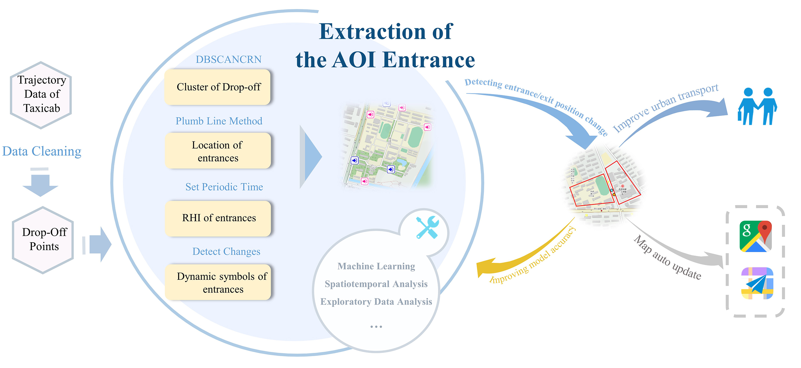
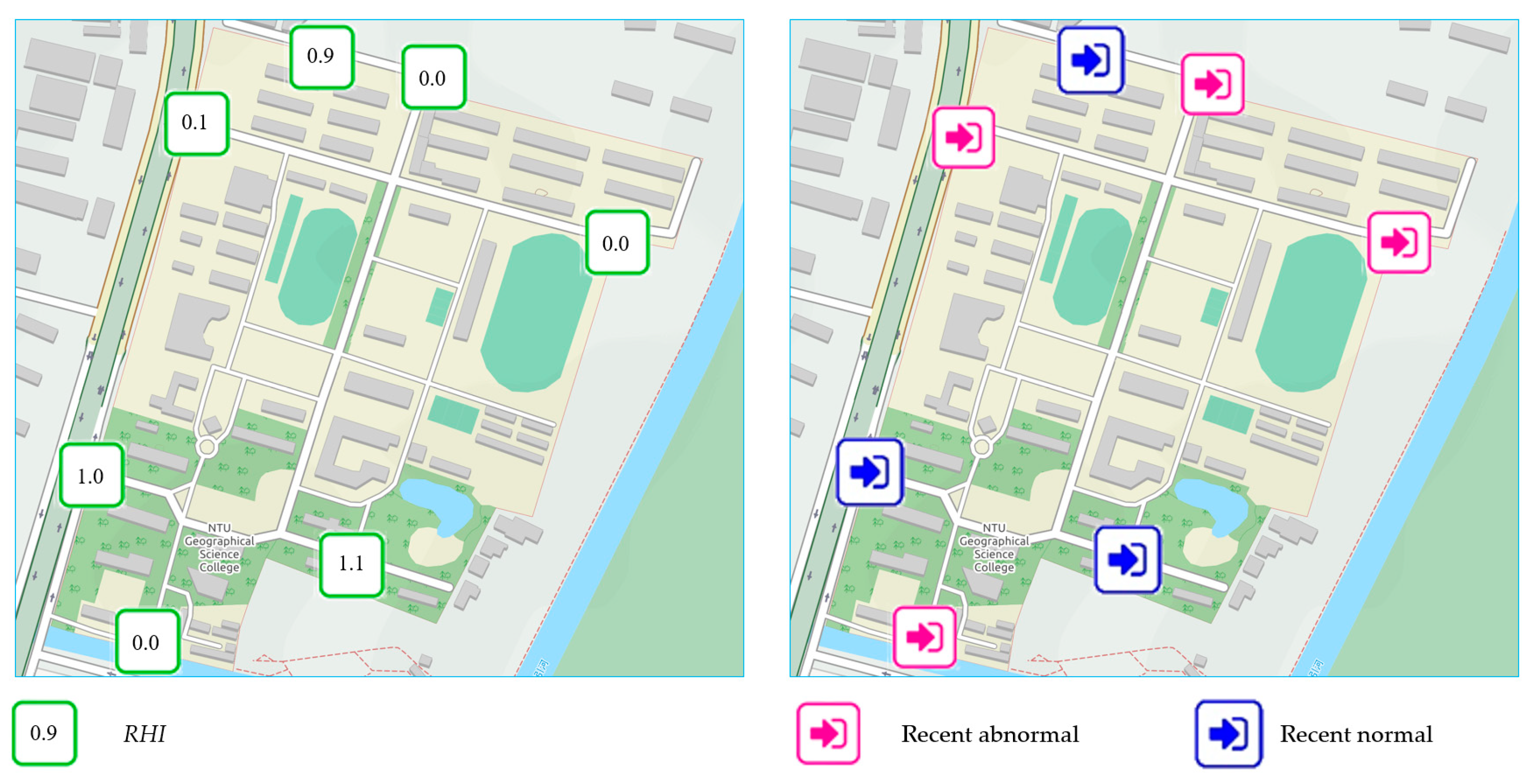
  • We propose a quantitative indicator to detect the access status of the entrance. Thus, it can enrich the expression of the map symbols, and then improve the navigation performance of the mobile map.
The rest of the article is organized as follows. The methodology of the article, as well as the related data and its preprocessing, is introduced in Section 2. The extraction process of the entrance location is presented in Section 3. Then, the accuracy and comparison analysis are illustrated in Section 4. The discussion follows in Section 5. Lastly, the conclusions and future work are in Section 6.

2. Methodology and Data Preprocessing

This article attempts to develop an approach to detect AOI entrances and their access status based on existing hardware and software conditions. In other words, new sensors and devices are not needed to solve this issue. There are many management information systems related to transportation in most cities in China, so the trajectory data of taxis can be collected all the time. If these data can be utilized in spatial mining effectively, it is undoubtedly a value-added service for the existing urban infrastructure.

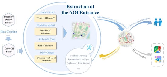
2.1. The Framework of the Research

There are several essential steps in this study: First, the taxi trajectory data are the primary experiment data, and the drop-off points are derived from these data. From this process, the cleaning of the drop-off points is a valuable finding in this article. Second, the drop-off points are partitioned under the constraint of the road network, and then, density-based classification is performed for each subset. To some extent, this approach reduces the limitation of the clustering method caused by uneven distribution. Then, the position of the entrance is calculated by the cluster center and AOI boundary. These operations are used to update the fundamental geographic data. Based on these, the temporal analysis of the clusters of the drop-off points is carried out for each entrance. The quantity change per unit time is used to detect the new access status of the entrances and further serve the visual optimization of the map symbols (Figure 2).

2.2. Data and Study Area

The experiments were conducted in the Chongchuan district of Nantong City, China. Nantong is located on the north bank of the Yangtze River estuary, of which gross domestic product (GDP) ranked 20th in the cities of China in 2018 [36]. The experimental data included taxi GPS trajectory and digital line graphic (DLG) thematic data. AOI and road network data in the same period were obtained using the Amap API by Web crawler technology. At the same time, a small number of aerial images from a drone were used for accuracy verification with a spatial resolution of 0.6 m.

2.2.1. Trajectory Data of Taxicab

The trajectory data of the taxicab covers the 31 days of October 2018, and the number of taxis was about 1400. Theoretically, the sampling time interval was 30 s but was less than 30 s in practice because the signal data caused by the change of the passenger status was also collected.
The raw taxi trajectory data used in this paper is in the xls file format and includes license plate number, phone number, time, longitude and latitude, speed, direction, and passenger status. License plate number and phone number are the unique identifiers of the taxi. Time represents the current date and time when obtained from the taxi. Latitude and Longitude contain the latitude and longitude coordinates of the taxi, respectively. Speed is a floating value that records the instantaneous velocity of the cab. Direction indicates the eight directions in which the vehicles were driving. Passenger status denotes whether a taxicab was occupied by passengers; it is a Boolean type variable with a value of 0 when the car was empty. An element of original sample data is recorded, as shown in Table 1.

2.2.2. AOI and Road Network Data

In the domain of GIS, AOI is a kind of geographic entity whose geometry style is the polygon and is usually used to describe the same geographical types of objects, such as hospitals, schools, and residents. Road network and AOI are often considered as a topological association or adjacent relationship, and the entrances are the connection between the road network and AOI. This means that if we partition the urban area into several blocks by road networks at a certain level, there is usually one or more AOI within each block.
In this paper, an AOI is defined as the tuple A = { A i , R i , N i } , where A i represents the index of the AOI, R i represents the i -th road around the AOI, and N i represents the i -th vertex of the AOI domain. There was a total of 48 AOIs with 63 entrances used in the experiments; AOI samples included 13 shopping malls, 5 scenic areas, 13 residential areas, 7 schools, and 5 hospitals. The details of area and number of drop-off points associated with the entrances are shown in Table 2.

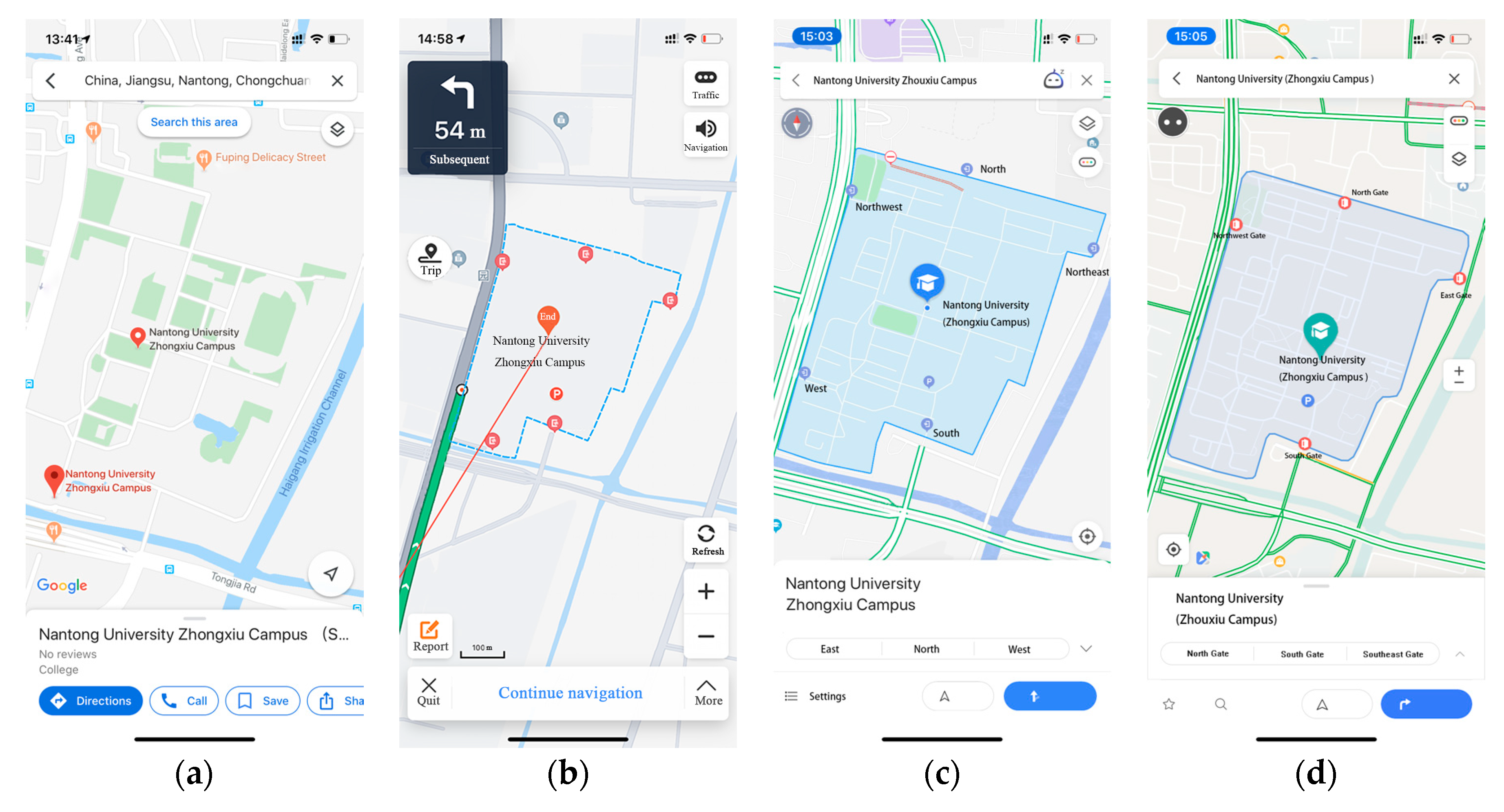
2.3. Cleaning of the Drop-Off Points

The spatial accuracy of trajectory data obtained through the BeiDou Navigation Satellite System (BDS) is about 5 to 10 m in the Asia-Pacific region. In theory, the signal point S P i can be acquired every 30 s during driving. Multiple sequential signal points can reflect the vehicle trajectory from S P 1 to S P n , as shown in Figure 3.
The trajectory data were cleaned to remove empty fields and obvious errors. Moreover, the drop-off points were cleaned in spatial accuracy for the following reasons.
Existing studies based on taxi trajectory are mostly oriented to the spatial granularity of the urban district or street level, and the spatial accuracy at the kilometer level can meet the need for research. However, the width of the entrance is usually less than 50 m. To extract the entrance position through the drop-off points, the spatial accuracy of the drop-off points should be less than 50 m.
When taxi drivers start or stop a new trip, the BDS device will record a signal point of the vehicle, which is marked with empty or heavy status, simultaneously. At the end of the trip, the passengers will be dropped at the destination. At the same time, the signal points that were collected by the BDS device will be recorded as drop-off points, as the set DP = { d p 1 , d p 2   ,…, d p n }. At present, almost all of the pick-up and drop-off points of taxis in relevant studies come from such signal points.
Existing studies regard the first signal point at the beginning of the trip order, which changes from heavy status to empty status, as the drop-off point. However, drivers may change the status of the taximeter in advance or continue driving until the vehicle has stopped for convenient operation. Therefore, there may be an error between the position of the signal point collected by the system and the real drop-off location. The error zone is shown in Figure 3.
Distance d i s s p i , s p i + 1 between heavy and empty status points can be calculated based on Equations (1) to (2).
a = arcsin ( [ sin ( S p i y S p i + 1 y 2 ) ] 2 + cos ( S p i y ) * cos ( S p i + 1 y ) * [ sin ( S p i x S p i + 1 x 2 ) ] 2 )
d i s s p i , s p i + 1 = 2 * a * 6371 * 1000
where S p i x represents the longitude of the i -th point, S p i y represents the latitude of the i -th point, and the variable i represents the sequence number of the point.
The radius width of the error zone may affect the extraction effect of the entrance. In this experiment, drop-off points that exceed 50 m accounted for about 23.5% of the whole data set (Figure 4). Moreover, the radius of a portion of data was larger than 100 m, which must affect the spatial accuracy of the extraction performance. In this paper, the average width of the associated road at the entrance, 50 m, was regarded as the threshold. After extraction, the trajectory points were cleaned again, and the drop-off points whose radius is greater than 50 m were removed.
The number of drop-off points was 1,048,575 before cleaning and 801,679 after cleaning, accounting for 76.5% of the original data. Through the cleaning processing, the number of entrances was reduced, and the distribution of drop-off points was relatively concentrated. The comparison of data before and after cleaning is shown in Figure 5.

3. The Extraction Process of the Entrances

The location of the AOI entrances was obtained through conventional manual survey, so the accuracy was higher than that of other methods. However, this approach consumes significant time and human resources, making it hard to achieve frequent updating of the entrances. A new approach is proposed in the following section.

3.1. Limitation of the Existing Methods

DBSCAN is a density-based clustering algorithm, which can separate high-density regions from low-density regions. The algorithm has two parameters, Eps and MinPts, which indicate the radius of the searching distance and number of points within the search area, respectively [34]. Then, the types of points are divided into three categories according to the above parameters. If the distance is less than Eps, and the number is higher than MinPts, the point is considered as a core point; otherwise, it is regarded as a boundary point, and other points are regarded as noise. The principle of the algorithm is to merge the key points whose distance is less than Eps, and the final result is a series of clusters and noise points. Density distribution is one of the key influencing factors of DBSCAN, which can be reflected by the settings of the two above parameters. For instance, Figure 6 shows two groups of DBSCAN clustering of simulated data sets with different Eps parameters. From the comparative experiments, we can find that a slight change of Eps may lead to a different result. The samples are divided into nine clusters in Figure 6a and three clusters in Figure 6b.

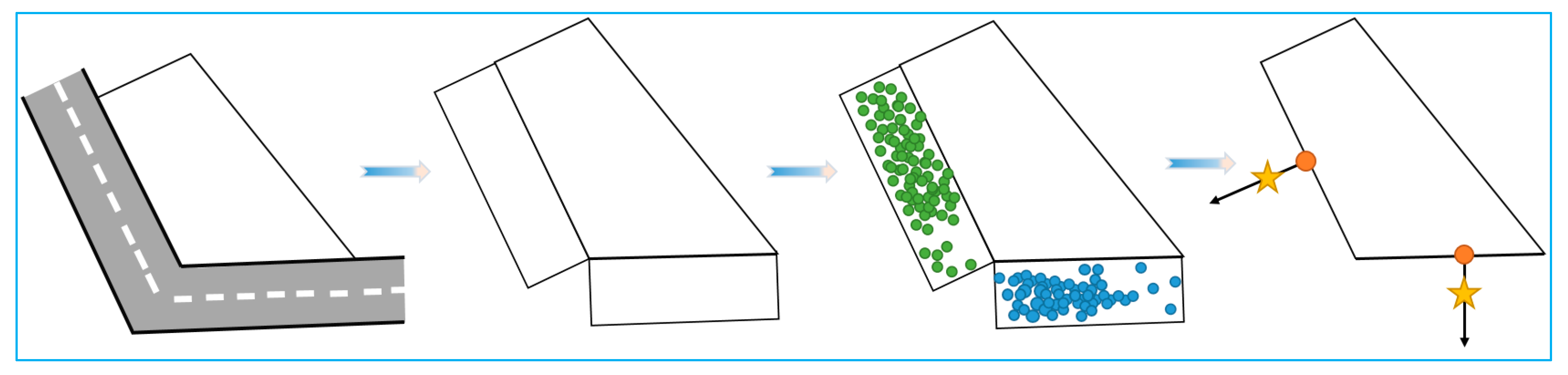
3.2. Extraction Approach for the AOI Entrances

Distribution of the drop-off points usually is affected by factors such as road width, land use type, the economic prosperity of AOI, and the shape of entrances, resulting in uneven status. It is difficult to mine the drop-off points using DBSCAN and K-means directly, due to the hierarchical uneven distribution. Therefore, this paper proposes an optimized spatial clustering approach, DBSCAN-Constrained by Roads Network (DBSCANCRN). The basic idea is to partition the drop-off points into pieces by road networks and search the road segments R i around each target AOI for the establishment of spatial relations and then cluster the drop-off points within each road segment separately. Based on the above operations, the location of the entrance is extracted by calculating the spatial relation between the clustering center and the associated road segment R i . The necessary process is shown in Figure 7.
The main steps are as follows:
1. Partition by road network
Road networks are used to divide urban areas. Generally, trajectory points are distributed in road segments, while AOIs are topologically contained in the grid polygon formed by road segments.
2. Spatial join of the AOI and roads
Entrances are the only way for residents to travel from AOIs to roads. In terms of spatial relationships, AOIs and road segments nearby can be regarded as spatial-association relationships. Therefore, AOI boundaries associated with roads can be selected to generate buffers on the outside of the boundaries. Because the drop-off points at the intersection of the road network can be attributed to many different road segments, this has a significant impact on the extraction of entrances. The rectangular area at the intersection of the road network is not considered; only other road segments are considered. The drop-off points in different buffer zones are recorded as set RC = { r c 1 , r c 2 ,…, r c n }.
3. Spatial clustering separately
The DBSCAN algorithm is applied to the drop-off point clusters in the set RC, and then the result is recorded as the set DB = { d b 1 , d b 2 , , d b n }. The points with a value of −1 are noise, and every other cluster corresponds to an AOI entrance. According to Equations (3) and (4), the coordinates of the center c e n n of each group d b n in the set DB are calculated.
c e n n x = i n p i x n
c e n n y = i n p i y n
where p i x represents the latitude of the i -th point and p i y represents the longitude of the i -th point.
4. Extraction of entrance positions
A vertical line is drawn through the cluster center and intersects the AOI boundary at a point, which is the location of the AOI entrance.
The pseudo-code of DBSCANCRN is shown in Algorithm 1.
Algorithm 1: Pseudo-code of the DBSCANCRN algorithm.
Input:Eps: the set of parameter Eps.
M: the set of parameter MinPts.
B: B = (P, j), where P is a data set containing drop-off points in B, and j is the index of B.
A: A = (B, i), where B is the buffer of the road associated with AOI, i is the index of AOI.
Output: set C of drop-off points.
begin
for each B in A
for each P in B
DBSCAN clustering of drop-off points in set P
end forend for
output C
end

4. Results and Analysis

To validate the effectiveness of the above algorithm, a series of experiments were conducted. The main findings and the analysis are presented in the following section.

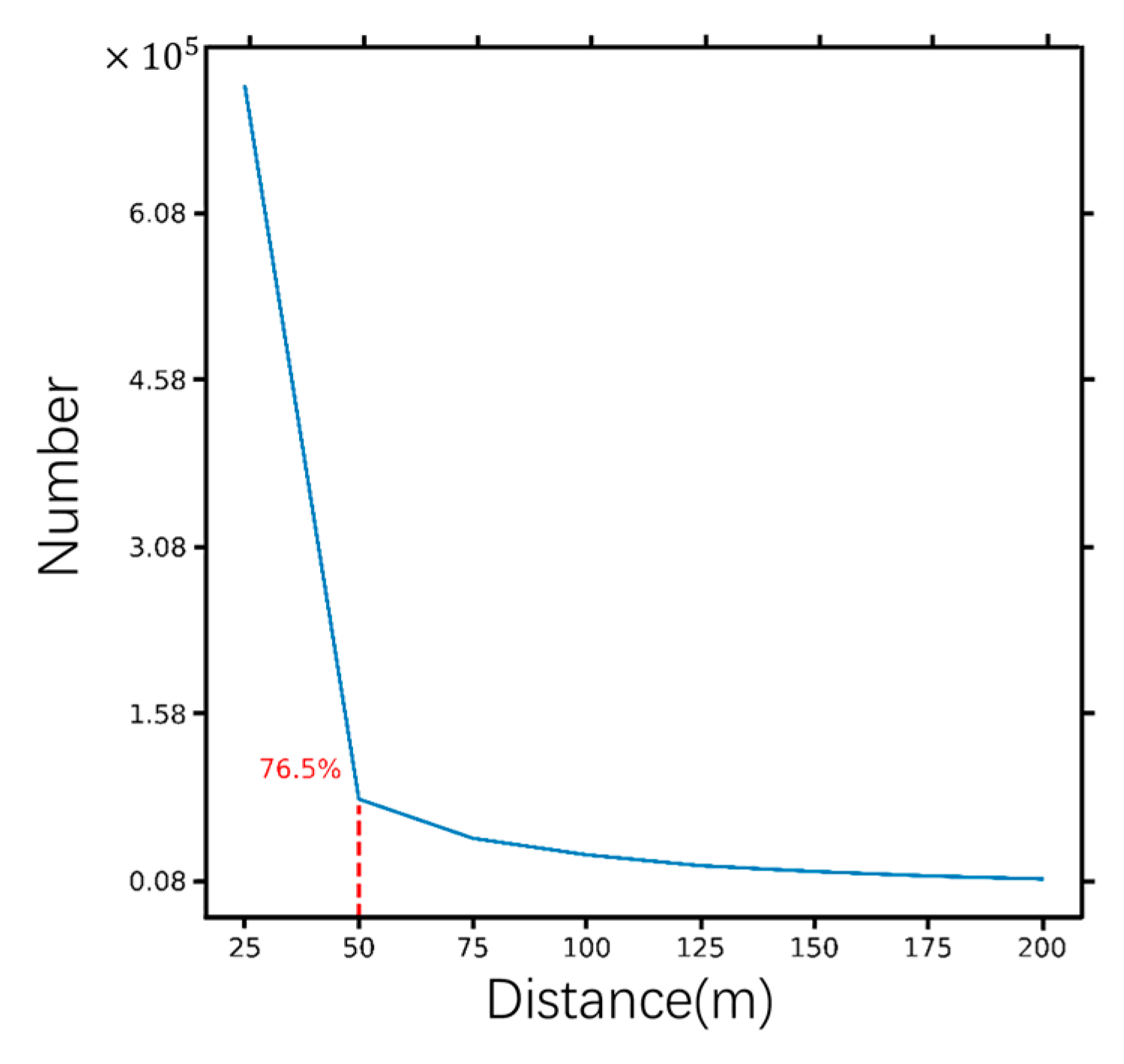
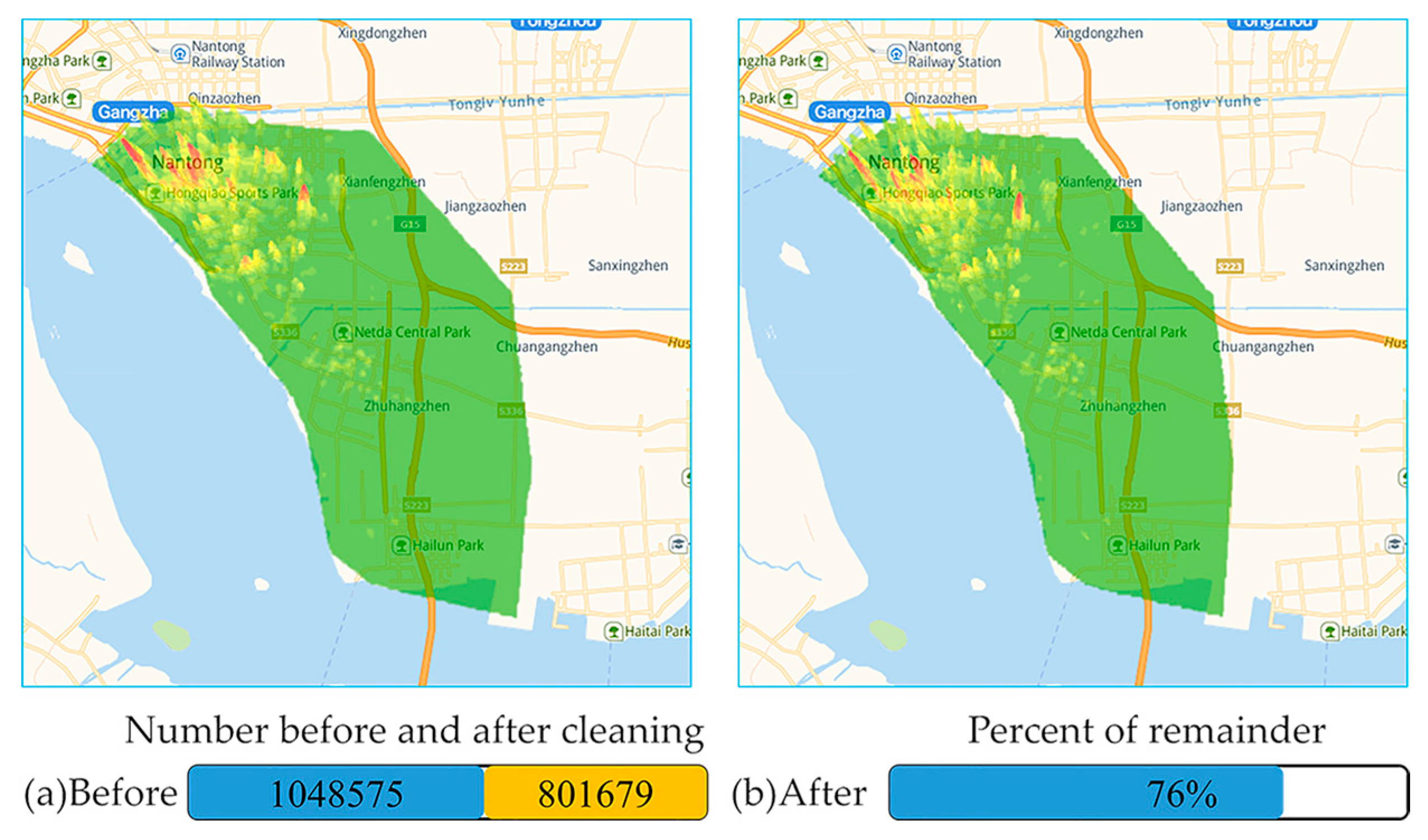
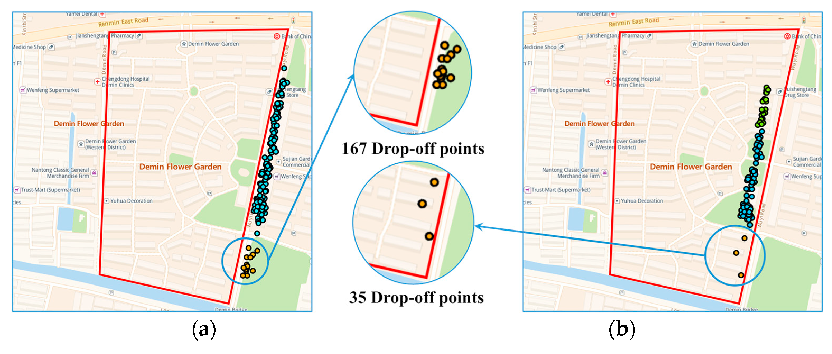
4.1. Cleaning Effect of the Drop-Off Points

The DBSCAN algorithm is sensitive to the density and distribution of sample points, so data cleaning is essential. When using uncleaned drop-off points to extract entrances, clustering results appear as abnormalities, and the number of clusters deviates significantly from the real position. Taking the Demin Huayuan District as an example, when clustering with uncleaned data, the drop-off points on the south-east side of the district are clustered into one group, but in fact, there is no entrance here. When 79% of the drop-off points are cleaned, the remaining points are judged as noise points due to their small number. The extraction results are consistent with the actual situation of the community, as shown in Figure 8.

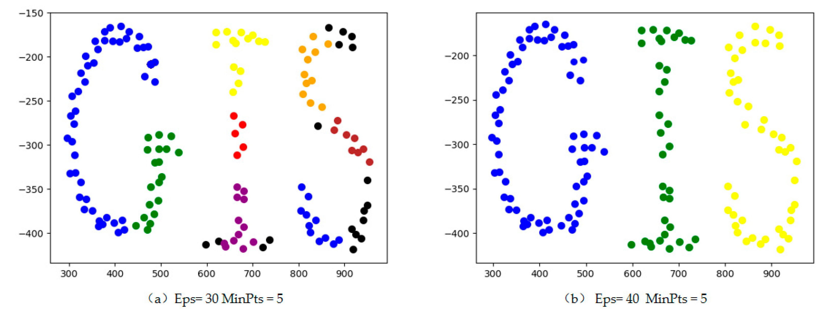
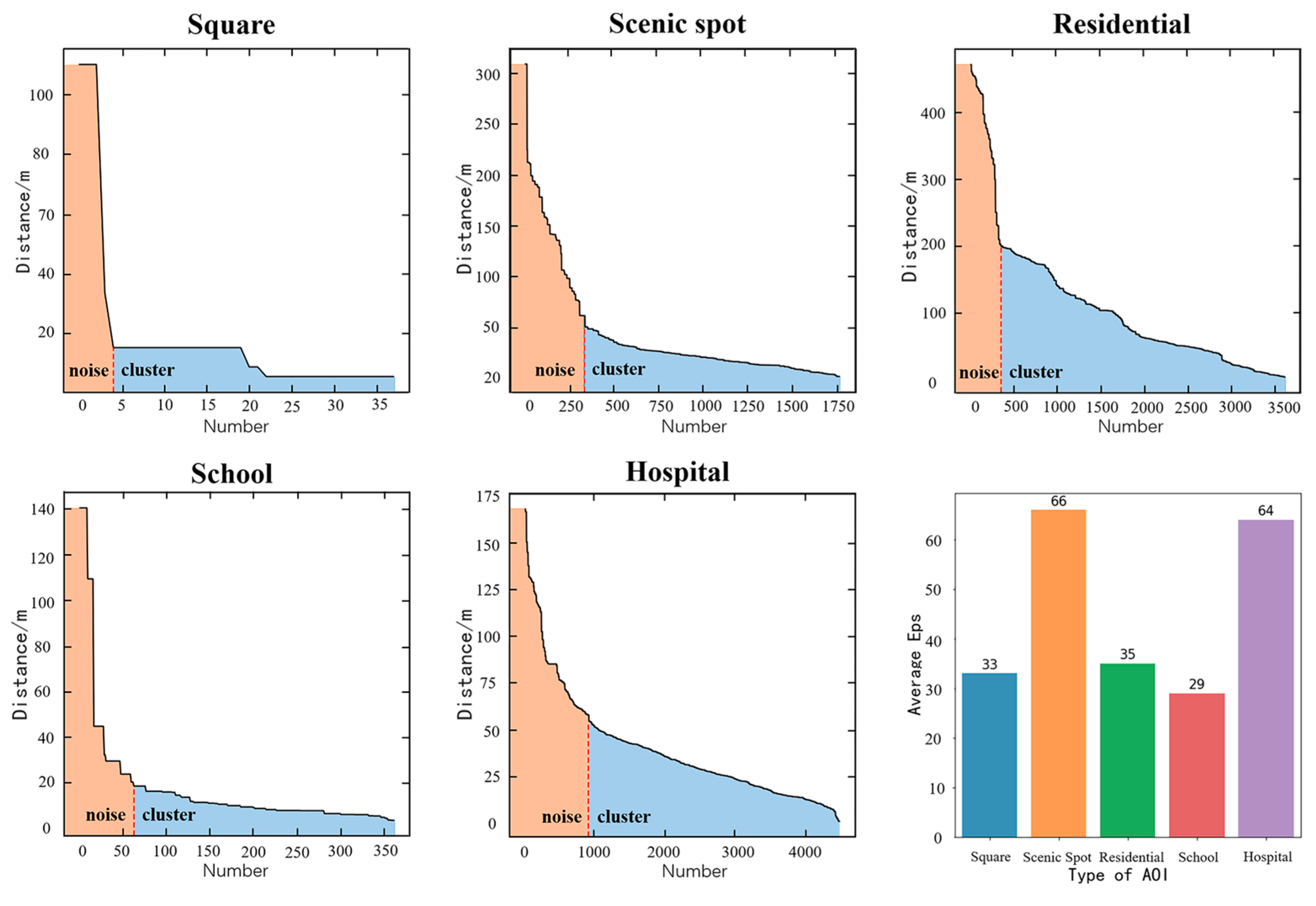
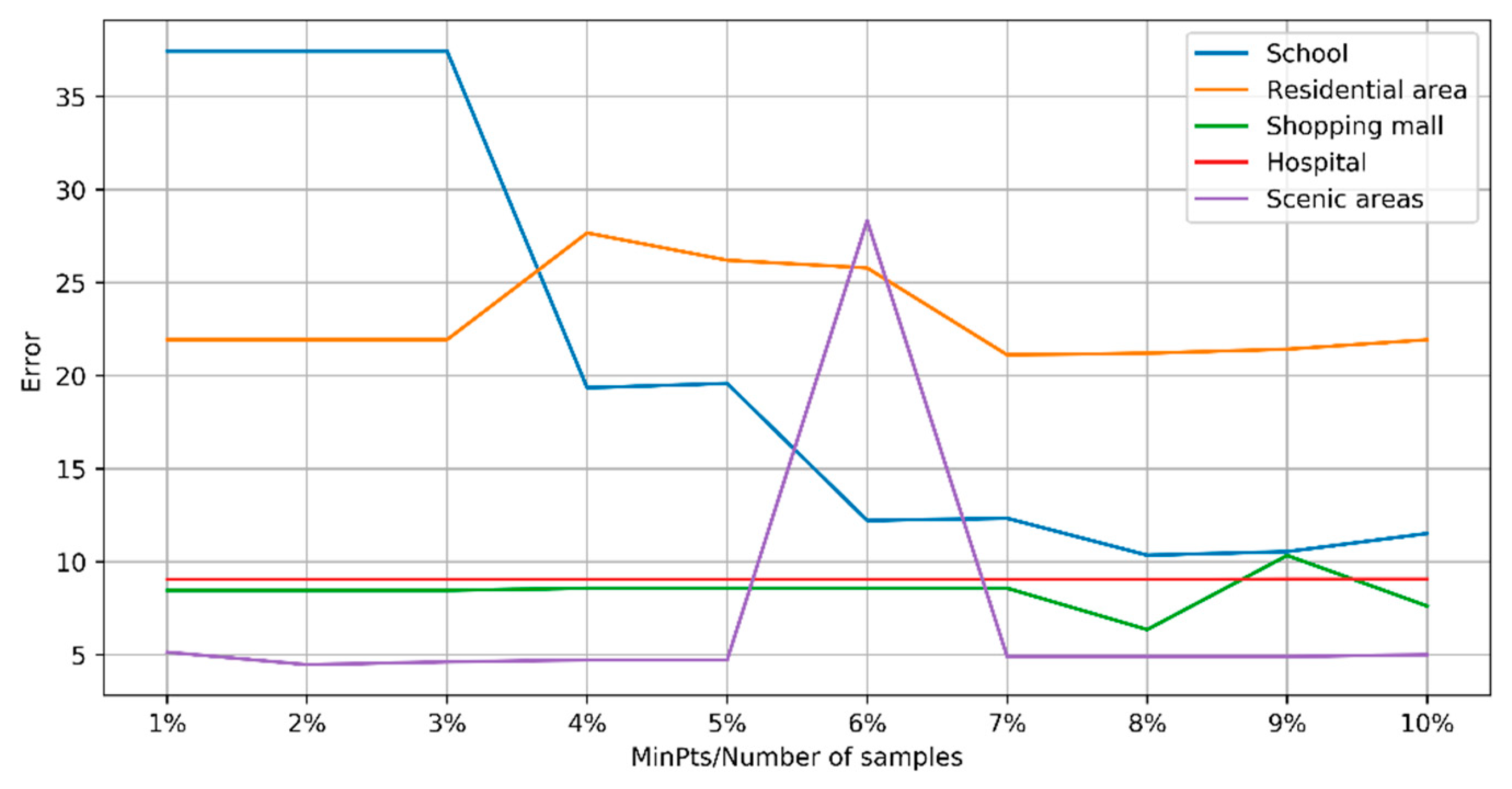
4.2. Parameter Setting of DBSCAN

Eps and MinPts are two critical parameters of the DBSCAN clustering algorithm. Previous experiments show that parameter setting has a significant impact on the results. To find a more reasonable and automated parameter setting approach, a series of experiments were conducted through cross-checking the drop-off points. It was found that the method proposed by Ester was still effective in the extraction experiments, which determines the value of radius Eps using the inflection point of the sorted K-nearest neighbor curve graph. When the value of K was 4 in his experiment, the effect was relatively stable [34]. The method was used in the experiments of this article.
The distances from all the drop-off points to the i-th point are arranged in descending order, and the graph is drawn to observe the mutation point. Setting Eps as the distance between the point P and the mutation point, the left point of the mutation point is identified as noise and the right as the core or boundary point. The Eps values of various AOIs are shown in Figure 9.
The value of MinPts heavily depends on the total number of drop-off points available in each AOI, so the MinPts can be set by adjusting the percentage, similar settings have been found very useful in detecting different types of urban areas of interest [37]. We set the MinPts from 1% to 10% in the calculation based on the above Eps, and the results of each type of AOI were shown as Figure 10; the value with the lowest error was selected as the best MinPts of each type of AOI.
The value of the Eps and the MinPts set in the experiment are shown in Table 3.

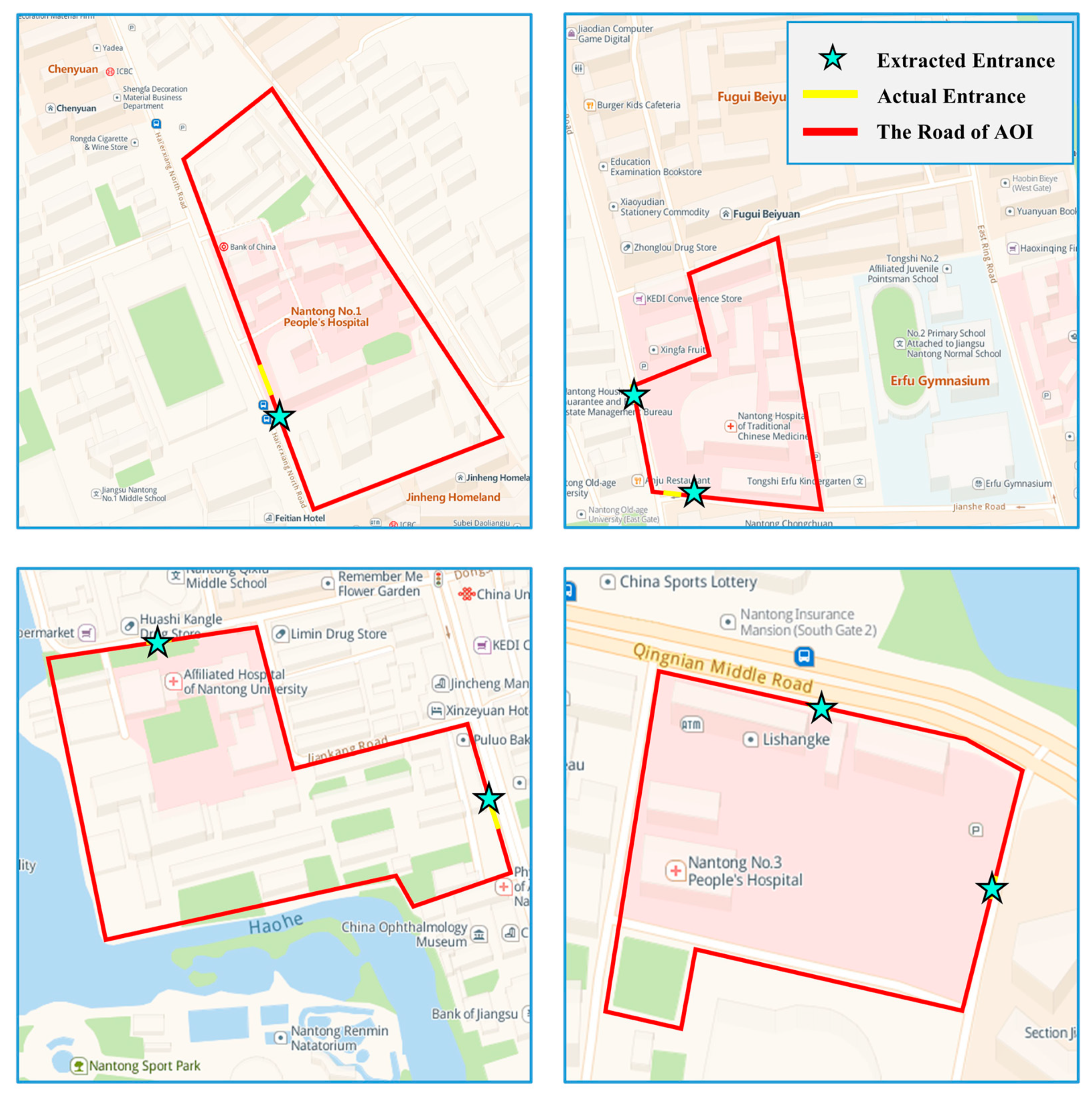
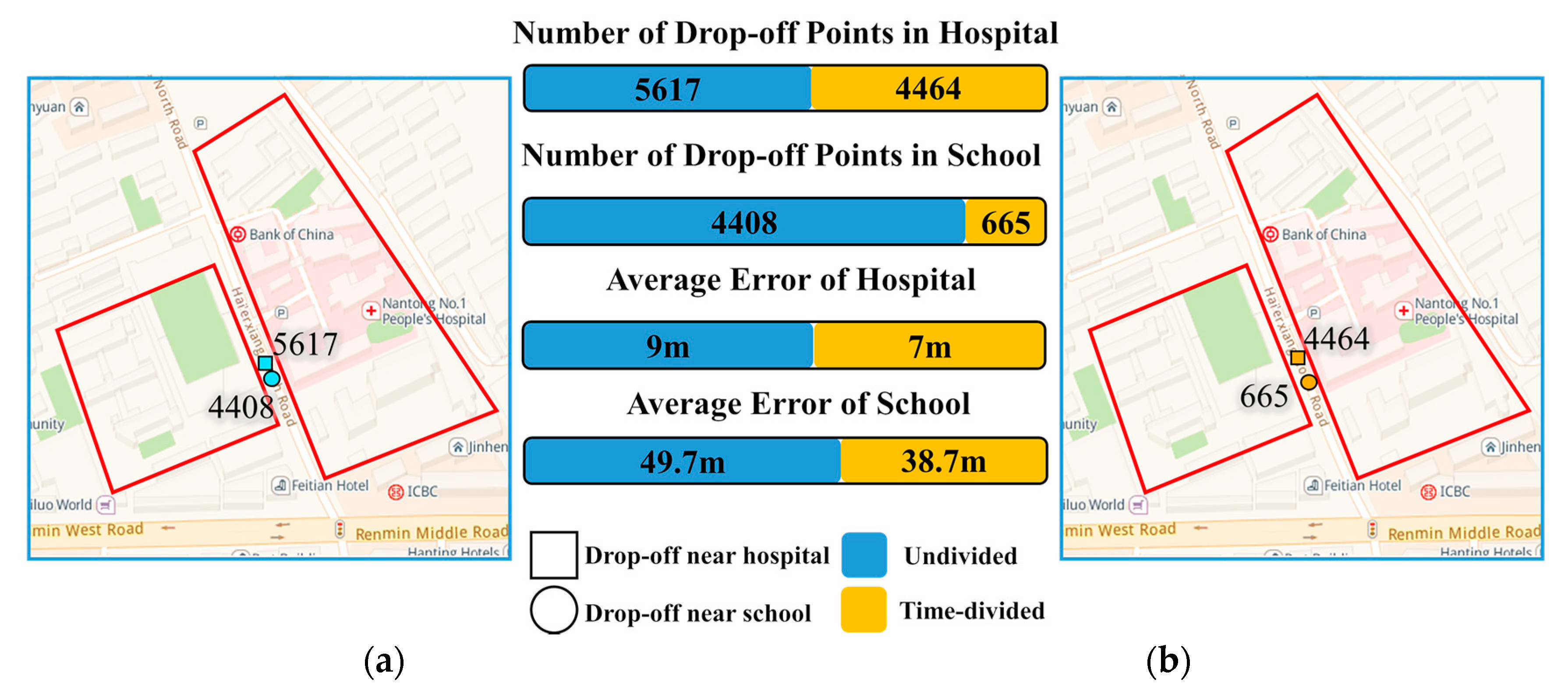
4.3. Accuracy of Extraction Results

In order to validate the precision of the extraction result, the extraction error was defined as the projection distance from the extracted position to the adjacent door of the real location, referring to the aerial image resolution of 0.6 m. Maps of four hospitals of Nantong City are shown in Figure 11; the error was expressed by the distance between the yellow and pentagram symbols.
The extraction errors of various types of AOI entrances are shown in Table 4.
The average error of the residential area is the largest one in Table 4, and the value is 22.4 m. The main reasons for the results are as follows: (1) An AOI with a nearby entrance has a cross-influence on the drop-off points; areas with the high pedestrian flow will affect the extraction results, and there may be mixed results of multiple AOI entrances. (2) Traffic regulations will affect location extraction of the drop-off points; one-way roads or parking restrictions on roads will lead to a deviation of the distance between drop-off points and entrances. (3) Open entrances are adopted in some shopping plazas, and taxis can enter the shopping plaza at will, which will result in relatively divergent locations of drop-off points. (4) Some residential districts’ AOIs near roads will also have a certain influence on the distribution of drop-off points. (5) Due to the different sources of geographic data, there are some errors in the process of coordinate registration, such as road network data deviating from the actual location and deforming.

4.4. Comparison with K-Means

K-means is an iterative clustering algorithm. Compared with the DBSCAN algorithm, it needs to determine the number of categories, K, in advance, and the shape of clustering results is relatively fixed. Because there are some differences in parameter setting between the two algorithms, K-means is used as the contrast to DBSCAN. This paper tries to compare the best clustering shape of each algorithm in order to reduce the impact of the threshold setting on the method. Therefore, the evaluation of the results is relatively objective. After associating the road with the AOIs, the drop-off points in the road segment were extracted and processed using the K-means clustering algorithm. The elbow method and silhouette coefficient were used to determine the parameter K in the K-means algorithm. When K calculated by the two methods was different, the K value with the smaller error was chosen for entrance extraction, as shown in Table 5.
On this basis, taking the south-east side of Xuetian Nanyuan District as an example, the K-means and DBSCANCRN methods were used to extract the entrances. The average extraction error of DBSCANCRN was 3.4 m, and the average error of K-means was 21.2 m (Figure 12).
The average accuracy of the K-means method is compared with that of DBSCANCRN. The results are shown in Table 6.
The average extraction error in the experimental sample area was 11.2 m, which was better than the average error of K-means of 17.3 m.
Although the average accuracy for the schools using DBSCAN was equal to K-Means, the error of DBSCANCRN for specific schools was larger than K-means. First, because No. 1 Middle School was close to No. 1 People’s Hospital, the entrances of them were adjacent. Moreover, the influence of No. 1 People’s Hospital was much significant, so the drop-off points were mainly distributed near it. Second, Some AOIs, such as Qi Xiu Campus and Nantong University Affiliated Normal Primary School, had a small number of drop-off points around due to the management style. The distribution of drop-off points was approximate even, and the DBSCAN was sensitive to density, under these circumstances, the extraction accuracy of K-Means was better than DBSCAN.

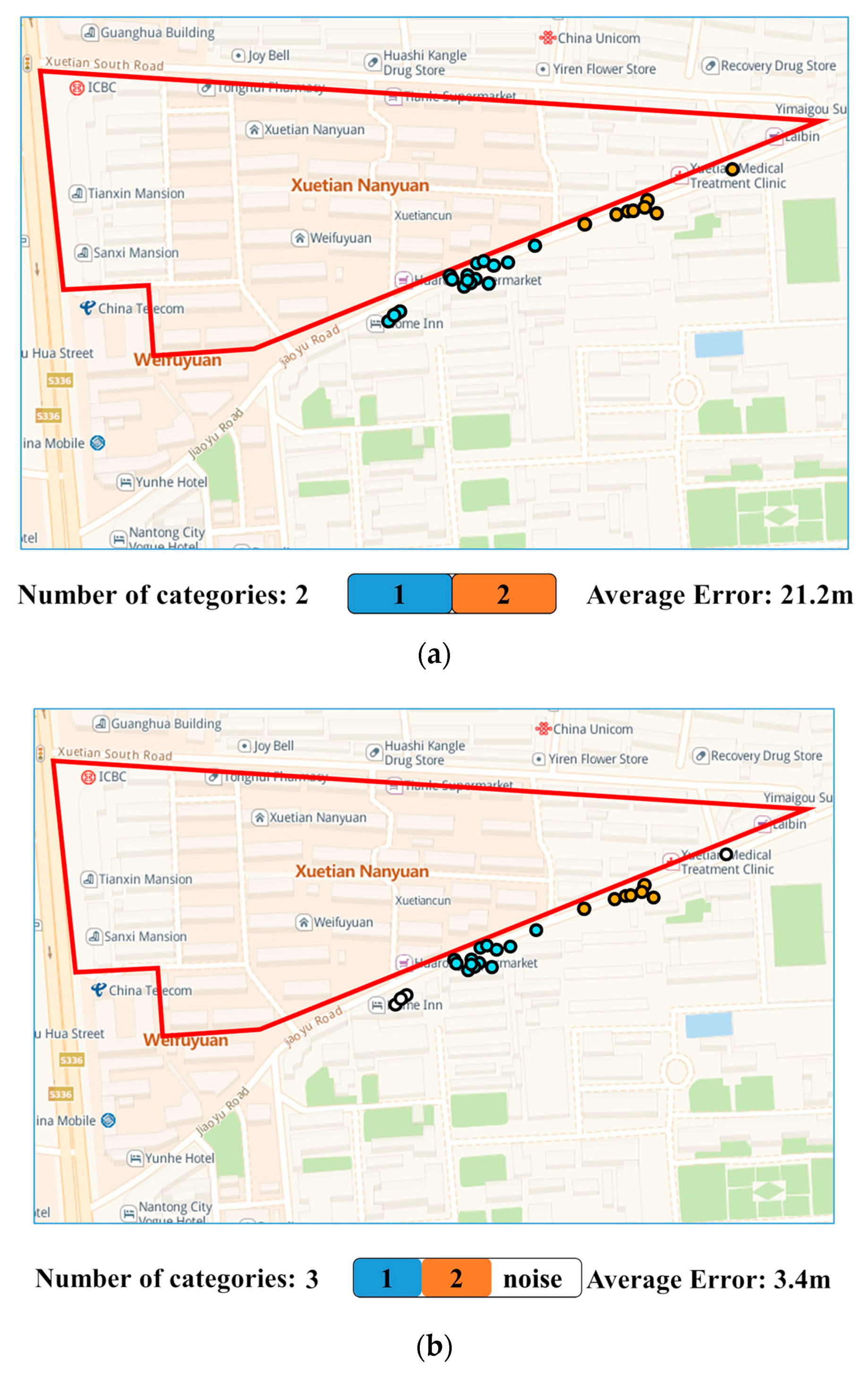
4.5. Processing of Special Case

There is mutual interference between the adjacent AOI, so it is impossible to determine which AOI area the passengers enter after leaving the taxi. Under this situation, it is hard to extract the entrances through the clustering of the drop-off points. To solve the above problem, this article designs a time-division method. Through analysis, it was found that 06:00–09:00 is the peak time of junior high school attendance. If the drop-off point cluster is divided into time segments, and the drop-off points in the peak period are assigned to the school, the extraction performance is significantly improved. For example, in the experiment, we take Nantong First Middle School and Nantong First People’s Hospital as examples. The two AOIs are distributed on the east and west sides of North Road of Children’s Lane, and have an influence on each other. If the drop-off point at 06:00–09:00 is selected to extract the entrances of First Middle School, and the remaining drop-off point is used to extract First People’s Hospital, the overall extraction effect is improved. In particular, the extraction accuracy of First Middle School in Nantong City is significantly improved, which shows that this method can reduce the interference of AOI to a certain extent. However, the accuracy of the hospital is decreased slightly, and further refinement of the operation is needed to achieve more satisfactory results, as shown in Figure 13, where orange denotes the time-divided drop-off points, and blue denotes the undivided points.

5. Discussion

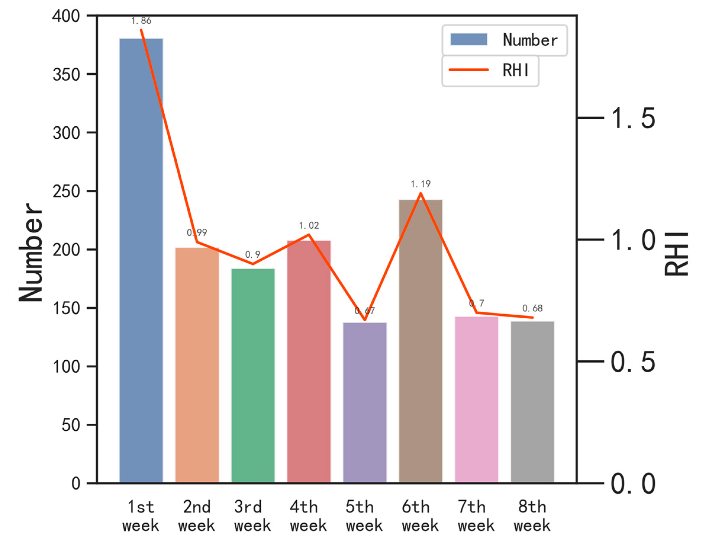
5.1. Application of Relative Hot Index

When the entrances are in normal status, the passenger flow will generally remain at a relatively stable level. Therefore, the number of AOI-related drop-off points can be used to measure the entrance status. However, due to the different flow rates at separate entrances, this paper proposes the R H I indicator, which can be used to measure the status change of entrances.
R H I = N u m c u r A v e ( N u m n )
where N u m c u r denotes the number of drop-off points in the current period, and A v e ( N u m n ) denotes the average of the past n periods. For example, regarding the week as the unit, when n = 4, if the number of the drop-off points is 888 this week and 1776 during the past four weeks, the R H I value is 2. Theoretically, the value of R H I should be around 1.0. If the value deviates significantly from 1.0, it indicates the abnormality of the entrance. When the R H I is too large, it can be judged that the entrance may be a hot spot, which may cause emergencies. Conversely, if an entrance occurs continuously with a small R H I , the entry may be temporarily closed.

5.2. Detection of Changes in Entrance Status by R H I

Entrances are correlated with drop-off points, and the heat of the entrance is measured by counting the number of related drop-off points. Taking the north gate of Zhongxiu Campus as an example, the drop-off points in October 2018 and the first week of May 2019 were selected to detect the changes in the entrance. Limited by the short period of acquisition of the experimental data, only one month’s calculation results are displayed. The heat of the entrance in October 2018 has a cycle of weeks, as shown in Figure 14.
The R H I value of the entrance in the first two weeks of May 2019 was also calculated. In the fourth week of October 2018, the number of drop-off points was 746, with an average R H I value of 1.0. In May 2019, the number of drop-off points was 0, and the average value was 0. It was speculated that the entrance may have an abnormal status, which was confirmed by field investigation: The entrance was closed in March 2019 due to construction on the outside of the building site, as shown in Figure 15.

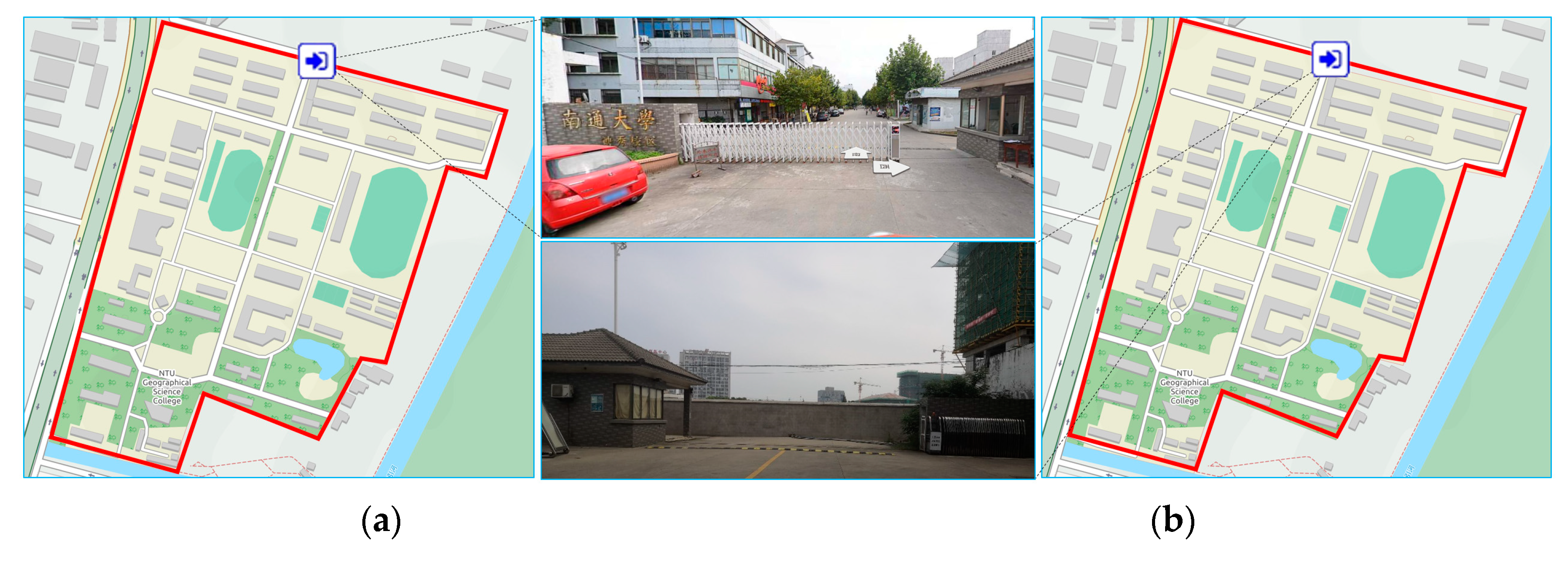
5.3. Aplication of the R H I

By setting the calculation period to monitor the access status dynamically, the R H I result of each entrance was obtained. According to the indicator, combined with manual verification, different types of map symbols can be designed, as shown in Figure 16b. Because the value is dynamic, the type of map symbols can be changed correspondingly when abnormal entrances change back to normal status.
However, in some extreme cases, there are still some limitations to this approach. In addition, the algorithm also depended on the number of drop-off points. Furthermore, the minimum time interval currently being done is one week, and it is difficult to discuss dynamic changes on a smaller time scale based on the current experimental condition.

6. Conclusions

This paper targets the dynamic monitoring of the access status (closed or open) of AOI entrances. Based on the existing trajectory data of taxicabs, an automatic solution was proposed. Firstly, fine-grained analysis of original taxi trajectory data was carried out, and a new data cleaning method was introduced, which can extract the drop-off points with higher spatial accuracy. Then, the modified DBSCANCRN was designed, which aids the determination of the parameters of the algorithm and enhances the extraction precision of the AOI entrances. Secondly, the location and quantity of the entrances and the drop-off points were correlated, and the R H I was calculated by the number of drop-off points in a period. Changes in the R H I can determine the access status of the entrance. The continuous operation of the approach will allow the detection of changes in entrances and instant notification of their access status and enhance sustainable urban transportation.

Author Contributions

Conceptualization, T.Z. and Z.Q.; methodology, T.Z. and X.L.; software, T.Z, Z.Q, and H.C.; validation, H.C.; formal analysis, Q.Z. and F.T.; writing—original draft preparation, T.Z., H.C., and Z.Q.; writing—review and editing, T.Z. and X.L.; visualization, Z.Q. and H.C.; supervision, F.T.; project administration, F.T.; funding acquisition, T.Z. and F.T.

Funding

This research was funded by the National Natural Science Foundation of China under Grant 41301514 and Grant 41401456, in part by the Nantong Key Laboratory Project under Grant CP12016005, in part by the National College Students Innovation and Entrepreneurship Training Program under Grant 201910304036Z, and in part by the Graduate Research and Innovation Projects of Jiangsu Province under Grant 201910304113Y.

Acknowledgments

The authors would like to thank the editor and the anonymous reviewers who provided insightful comments on improving this article and The Hong Kong Polytechnic University for providing the opportunity of academic exchange. We also thank Rong Tsao, Research Scientist of Agriculture and Agriculture-Food Canada, for his valuable advice on the improvement of English writing.

Conflicts of Interest

The authors declare no conflict of interest.

References

  1. Talebi, M.; Vafaei, A.; Monadjemi, A. Vision-based entrance detection in outdoor scenes. Multimed. Tools Appl. 2018, 77, 26219–26238. [Google Scholar] [CrossRef]
  2. Liu, J.; Korah, T.; Hedau, V.; Parameswaran, V.; Grzeszczuk, R.; Liu, Y. Entrance detection from street-view images. In Proceedings of the IEEE International Conference on Computer Vision and Pattern Recognition Workshop (CVPR), Columbus, OH, USA, 24–27 June 2014; pp. 1–2. [Google Scholar]
  3. Zhang, Y.; Luo, H.; Skitmore, M.; Li, Q.; Zhong, B. Optimal Camera Placement for Monitoring Safety in Metro Station Construction Work. J. Constr. Eng. Manag. 2018, 145, 04018118. [Google Scholar] [CrossRef] [Green Version]
  4. Ding, L.; Fang, W.; Luo, H.; Love, P.E.; Zhong, B.; Ouyang, X. A deep hybrid learning model to detect unsafe behavior: Integrating convolution neural networks and long short-term memory. Autom. Constr. 2018, 86, 118–124. [Google Scholar] [CrossRef]
  5. Yue, Y.; Zhuang, Y.; Yeh, A.G.; Xie, J.Y.; Ma, C.L.; Li, Q.Q. Measurements of POI-based mixed use and their relationships with neighbourhood vibrancy. Int. J. Geogr. Inf. Sci. 2017, 31, 658–675. [Google Scholar] [CrossRef] [Green Version]
  6. Goodchild, M.F.; Li, L. Assuring the quality of volunteered geographic information. Spat. Stat. 2012, 1, 110–120. [Google Scholar] [CrossRef]
  7. Zhou, T.; Shi, W.; Liu, X.; Tao, F.; Qian, Z.; Zhang, R. A Novel Approach for Online Car-Hailing Monitoring Using Spatiotemporal Big Data. IEEE Access 2019, 7, 128936–128947. [Google Scholar] [CrossRef]
  8. Su, R.; Fang, Z.; Luo, N.; Zhu, J. Understanding the dynamics of the pick-up and drop-off locations of taxicabs in the context of a subsidy war among e-hailing apps. Sustainability 2018, 10, 1256. [Google Scholar] [CrossRef] [Green Version]
  9. Huang, L.; Wen, Y.; Ye, X.; Zhou, C.; Zhang, F.; Lee, J. Analysis of spatiotemporal trajectories for stops along taxi paths. Spat. Cogn. Comput. 2018, 18, 194–216. [Google Scholar] [CrossRef]
  10. Zheng, L.; Xia, D.; Zhao, X.; Tan, L.; Li, H.; Chen, L.; Liu, W. Spatial–temporal travel pattern mining using massive taxi trajectory data. Phys. A 2018, 501, 24–41. [Google Scholar] [CrossRef]
  11. Rossi, A.; Barlacchi, G.; Bianchini, M.; Lepri, B. Modelling Taxi Drivers’ Behaviour for the Next Destination Prediction. IEEE Trans. Intell. Transp. Syst. 2019, 1–10. [Google Scholar] [CrossRef]
  12. Brockmann, D.; Hufnagel, L.; Geisel, T. The scaling laws of human travel. Nature 2006, 439, 462–465. [Google Scholar] [CrossRef] [PubMed]
  13. Gonzalez, M.C.; Hidalgo, C.A.; Barabasi, A.L. Understanding individual human mobility patterns. Nature 2008, 453, 779–782. [Google Scholar] [CrossRef] [PubMed]
  14. Song, C.; Qu, Z.; Blumm, N.; Barabási, A.L. Limits of predictability in human mobility. Science 2010, 327, 1018–1021. [Google Scholar] [CrossRef] [PubMed] [Green Version]
  15. Liang, X.; Zheng, X.; Lv, W.; Zhu, T.; Xu, K. The scaling of human mobility by taxis is exponential. Phys. A 2012, 391, 2135–2144. [Google Scholar] [CrossRef] [Green Version]
  16. Guerra, C.A.; Kang, S.Y.; Citron, D.T.; Hergott, D.E.B.; Perry, M.; Smith, J.; Phiri, W.P.; Osa Nfumu, J.O.; Mba Eyono, J.N.; Battle, K.E.; et al. Human mobility patterns and malaria importation on Bioko Island. Nat. Commun. 2019, 10, 2332. [Google Scholar] [CrossRef] [PubMed] [Green Version]
  17. Jasny, B.R.; Stone, R. Prediction and its limits. Science 2017, 355, 468–469. [Google Scholar] [CrossRef] [Green Version]
  18. Zhong, R.; Luo, J.; Cai, H.; Sumalee, A.; Yuan, F.; Chow, A.H. Forecasting journey time distribution with consideration to abnormal traffic conditions. Transp. Res. C Emerg. Technol. 2017, 85, 292–311. [Google Scholar] [CrossRef]
  19. Jiang, S.; Guan, W.; He, Z.; Yang, L. Measuring Taxi Accessibility Using Grid-Based Method with Trajectory Data. Sustainability 2018, 10, 3187. [Google Scholar] [CrossRef] [Green Version]
  20. Chen, C.; Jiao, S.; Zhang, S.; Liu, W.; Feng, L.; Wang, Y. TripImputor: Real-time imputing taxi trip purpose leveraging multi-sourced urban data. IEEE Trans. Intell. Transp. Syst. 2018, 19, 3292–3304. [Google Scholar] [CrossRef]
  21. Liu, X.; Gong, L.; Gong, Y.; Liu, Y. Revealing travel patterns and city structure with taxi trip data. J. Transp. Geogr. 2015, 43, 78–90. [Google Scholar] [CrossRef] [Green Version]
  22. Yang, Z.; Franz, M.L.; Zhu, S.; Mahmoudi, J.; Nasri, A.; Zhang, L. Analysis of Washington, DC taxi demand using GPS and land-use data. J. Transp. Geogr. 2018, 66, 35–44. [Google Scholar] [CrossRef]
  23. Yue, Y.; Wang, H.D.; Hu, B.; Li, Q.Q.; Li, Y.G.; Yeh, A.G. Exploratory calibration of a spatial interaction model using taxi GPS trajectories. Comput. Environ. Urban Syst. 2012, 36, 140–153. [Google Scholar] [CrossRef]
  24. Tang, L.; Zhao, Y.; Cabrera, J.; Ma, J.; Tsui, K.L. Forecasting Short-Term Passenger Flow: An Empirical Study on Shenzhen Metro. IEEE Trans. Intell. Transp. Syst. 2018, 20, 3613–3622. [Google Scholar] [CrossRef]
  25. Zhao, P.; Liu, X.; Shen, J.; Chen, M. A network distance and graph-partitioning-based clustering method for improving the accuracy of urban hotspot detection. GeoIn 2017, 34, 293–315. [Google Scholar] [CrossRef]
  26. Tang, L.; Kan, Z.; Zhang, X.; Sun, F.; Yang, X.; Li, Q. A network Kernel Density Estimation for linear features in space–time analysis of big trace data. Int. J. Geogr. Inf. Sci. 2015, 30, 1717–1737. [Google Scholar] [CrossRef]
  27. Parzen, E. On estimation of a probability density function and mode. Ann. Math. Stat. 1962, 33, 1065–1076. [Google Scholar] [CrossRef]
  28. Getis, A.; Ord, J.K. The analysis of spatial association by use of distance statistics. In Perspectives on Spatial Data Analysis; Springer: Berlin/Heidelberg, Germany, 2010; pp. 127–145. [Google Scholar]
  29. Ord, J.K.; Getis, A. Local spatial autocorrelation statistics: Distributional issues and an application. Geogr. Anal. 1995, 27, 286–306. [Google Scholar] [CrossRef]
  30. Deng, M.; Yang, X.; Shi, Y.; Gong, J.; Liu, Y.; Liu, H. A density-based approach for detecting network-constrained clusters in spatial point events. Int. J. Geogr. Inf. Sci. 2018, 33, 466–488. [Google Scholar] [CrossRef]
  31. Hu, C.; Thill, J.C. Predicting the Upcoming Services of Vacant Taxis near Fixed Locations Using Taxi Trajectories. ISPRS Int. J. Geo-Inf. 2019, 8, 295. [Google Scholar] [CrossRef] [Green Version]
  32. Shen, J.; Liu, X.; Chen, M. Discovering spatial and temporal patterns from taxi-based Floating Car Data: A case study from Nanjing. GISci. Remote Sens. 2017, 54, 617–638. [Google Scholar] [CrossRef]
  33. Hartigan, J.A.; Wong, M.A. Algorithm AS 136: A k-means clustering algorithm. J. R. Stat. Soc. Ser. C Appl. Stat. 1979, 28, 100–108. [Google Scholar] [CrossRef]
  34. Ester, M.; Kriegel, H.P.; Sander, J.; Xu, X. A Density-Based Algorithm for Discovering Clusters in Large Spatial Databases with Noise. In Kdd; AAAI Press: Portland, OR, USA, 1996. [Google Scholar]
  35. Tang, J.; Liu, F.; Wang, Y.; Wang, H. Uncovering urban human mobility from large scale taxi GPS data. Phys. A 2015, 438, 140–153. [Google Scholar] [CrossRef]
  36. Zhou, S.; Zhai, G.; Shi, Y. What Drives the Rise of Metro Developments in China? Evidence from Nantong. Sustainability 2018, 10, 2931. [Google Scholar] [CrossRef] [Green Version]
  37. Hu, Y.; Gao, S.; Janowicz, K.; Yu, B.; Li, W.; Prasad, S. Extracting and understanding urban areas of interest using geotagged photos. Computers. Environ. Urban Syst. 2015, 54, 240–254. [Google Scholar] [CrossRef]
Figure 1. Map visualization of mainstream navigation apps: (a) Google Maps; (b) Baidu Maps; (c) Amap; and (d) Tencent Maps.
Sustainability 11 06870 g001
Figure 2. Framework chart of this research. In the flow, the cleaning of the drop-off points, the location extraction of the entrances, and the relative hot index ( R H I ) indicator are the three main innovations of this article.
Sustainability 11 06870 g002
Figure 3. Error zone of the drop-off points; the red circle symbols denote the empty status, and larger circles indicate the drop-off points.
Sustainability 11 06870 g003
Figure 4. Percentage chart of the number distribution about the locational error of the drop-off points during the cleaning process.
Sustainability 11 06870 g004
Figure 5. Distribution of the drop-off points: (a) Before cleaning, the number was 1,048,575, and the distribution was more scattered; (b) after cleaning, distribution was relatively concentrated.
Sustainability 11 06870 g005
Figure 6. Classification results of simulated data by the DBSCAN algorithm under the different parameter settings. (a) Classification performance failed to achieve the desired results due to inappropriate parameters; (b) after improving the parameters set, the object can be detected.
Sustainability 11 06870 g006
Figure 7. Flow chart of AOI entrance extraction; the green and blue dots denote the drop-off points, the pentagram symbols represent the center of the cluster of the drop-off points, and the orange dots denote the calculated location of the entrance.
Sustainability 11 06870 g007
Figure 8. Cleaning effect of the drop-off points.
Sustainability 11 06870 g008
Figure 9. K-distance curves of various kinds of AOI.
Sustainability 11 06870 g009
Figure 10. The relation between the error and the MinPts.
Sustainability 11 06870 g010
Figure 11. Extraction results of the main hospitals in the study area. The pentagram symbols denote the position by calculating the drop-off points, and the yellow line symbols denote the real location.
Sustainability 11 06870 g011
Figure 12. Comparison of the extraction results between DBSCANCRN and K-means: (a) K-means clustering extraction results; (b) DBSACNCRN clustering extraction results.
Sustainability 11 06870 g012
Figure 13. Comparison of the drop-off points before and after time division. Orange denotes the drop-off points are time-divided and blue denotes the undivided ones.
Sustainability 11 06870 g013
Figure 14. The R H I of north gate of Zhongxiu Campus in September and October 2018.
Sustainability 11 06870 g014
Figure 15. Comparison before and after closing the north gate of Zhongxiu Campus in October 2018 and May 2019.
Sustainability 11 06870 g015
Figure 16. R H I and classified map symbols diagram: (a) R H I results; (b) classified map symbols.
Sustainability 11 06870 g016
Table 1. Partial trajectory data record.
License Plate NumberPhone NumberTimeLatitude and Longitude (°)Speed (km/h)DirectionPassenger Status
Su F*78139****34742018/10/2120.84786342.6positive south0
0:00:0032.021630
Su F*78139****34742018/10/2120.84914341.9positive south0
0:00:3032.018836
Su F*78139****34742018/10/2120.8498810positive south0
0:01:0032.017181
Su F*78139****34742018/10/3120.88679626.9positive south1
23:59:0031.987893
Su F*78139****34742018/10/3120.88756753.8positive south1
23:59:3031.984338
Table 2. Information of partial AOI samples.
Type of AOINumber of AOIAOI NameArea (km2)Number of Drop-Off Points
Shopping mall13Outlets Shopping Square0.049200
Gold Coast International Square0.072479
Hongming Mall0.063489
Darunfa Supermarket0.103457
Zhongnan Shopping Mall0.0573464
Scenic area5Nantong Exploration Kingdom0.3971759
Haohe Museum0.026909
Nantong Museum0.094422
Sports Park0.0733777
The Undersea World0.432548
Residential area13The north Community0.027171
Beiguo Community0.096313
Demin Garden0.2471198
Chunhui Garden0.3211535
Zhongnan Century Garden0.259732
School7Nantong No.1 Middle School0.0314408
Qixiu campus of Nantong University0.201169
Nantong Vocational University0.1751436
Nantong Technical College0.2291997
Nantong Technical Vocational College0.2611375
Hospital5Nantong No.1 People’s Hospital0.0425438
Nantong Hospital of Traditional Chinese Medicine0.0251427
Affiliated Hospital of Nantong University0.09510784
Nantong No.3 People’s Hospital0.0745919
Great Wall Hospital of Nantong0.007688
Table 3. The value of the Eps and the MinPts in the experiment.
Type of AOIEps (m)MinPts (%)
School338
Hospital668
Scenic areas352
Shopping mall298
Residential area647
Table 4. The extraction errors of entrances from typical kinds of AOI.
IDShopping MallScenic AreaResidential AreaSchoolHospital
Error (m)Area (km2)Error (m)Area (km2)Error (m)Area (km2)Error (m)Area (km2)Error (m)Area (km2)
10.00.0490.00.3973.30.02749.70.0318.80.042
20.00.0492.00.0266.50.09612.90.2010.00.025
313.30.07211.90.0942.20.2474.30.1758.30.025
40.00.0722.50.094135.30.1140.00.1753.80.095
50.00.06310.40.073110.1140.00.4193.40.095
65.50.0630.00.43216.70.1140.01.79342.60.074
72.20.088//17.40.2121.31.7930.00.074
836.40.088//24.80.59401.7935.30.007
90.00.088//280.04922.30.103//
105.80.043//21.10.11913.40.229//
1110.90.046//39.60.1193.20.229//
120.00.046//9.50.20117.10.261//
1312.80.031//10.00.354////
141.20.348//31.10.354////
156.40.019//21.80.181////
167.50.016//00.321////
170.00.055//1.80.259////
181.70.103//00.259////
1911.00.057////////
2012.40.057////////
Table 5. Comparison of elbow method and silhouette coefficient.
K of Elbow Method K of Silhouette CoefficientError of Elbow Method (m)Error of Silhouette Coefficient (m)The Best K Minimum Error (m)
Outlets Shopping Plaza294.76.724.7
Nantong Museum222.62.622.6
De min Garden2486.555.7455.7
Nantong Vocational University2414.235.5214.2
Nantong Hospital of Traditional Chinese Medicine222323223
Table 6. Comparison of the average errors of the two methods.
TypeError (m)
DBSCANCRNK-MEANS
School10.410.4
Hospital9.022.6
Scenic areas4.54.6
Shopping mall6.411.9
Residential area21.129.9

