1. Introduction
With rich water resources, basins have become core areas of human social and economic development [
1]. However, the integrity of catchment areas in basins has always been divided by artificial administrative areas, which results in the separation of water resource utilization and drainage activities planning and management [
2]. This division has led to conflicts in the allocation of water resources and the total pollutant load [
3], which not only reduce the overall water use efficiency, but also exacerbate the crisis of pollution in basins [
4]. Water resource limitations and environmental capacities in basins and the continually increasing demand for socioeconomic development have made this contradiction sharper and more severe [
5]. Therefore, the rational and equitable allocation of water resources and the pollutant loads between upstream and downstream areas is key for solving the problem of interregional conflicts and water crises and pollution.
The water resources and environmental capacities of basins have the attributes of quasi-public goods, and the externalities of water use and discharge activities are the causes of interregional conflicts [
6]. The allocations of water resources and pollutant loads in basins are multiattribute and multiobjective decisions [
7], which need to consider the hydrosystems and socioeconomic systems in basins and satisfy each stakeholder as much as possible. Beginning with reservoir optimization scheduling studies in the 1940s, the early allocations of water resources and pollutant loads in basins were based on the assumption of collective rationality following the principles of security, fairness, and efficiency, and various hydrological models (e.g., [
7]) and multiobjective optimization models (e.g., [
8]) were established for allocating water resources and pollutant loads among different regions and sectors within basins, which are known as the ‘top-down’ type. With sufficient water resources and environmental capacities, stakeholders can recognize and implement these optimized allocation schemes. However, as the scale of population and economy in a basin continue to expand, water use and pollutant discharge conflicts among different agents (regions and sectors) also escalate. The traditional ‘top-down’ optimization allocation cannot meet the upstream and downstream requirements, and the implementation of the allocation plan has no guarantee [
9].
The application of game theory, bankruptcy theory, social choice theory, and fallback bargaining for the allocation of water resources and pollutant loads in basins make allocations from the perspective of interaction and negotiation, which ensures that the preferences of various stakeholders are met and the allocation plans are implemented [
10,
11]. The models that are based on game theory focus on the equilibrium characteristic of decision-making when the activities of stakeholders interact [
12], such as the graph model for water resource conflict resolution developed by [
13], the cooperative and noncooperative allocation model that was designed by [
14], and the weighing factors model for equitable and reasonable allocation that was proposed by [
15]. Bankruptcy theory is a method of distributing surplus assets of enterprises, and it is used to distribute the residual value of an enterprise among creditors when it goes bankrupt (which is always insolvent). When the theory is applied to solve water resources and environmental conflicts, the limited water resource availability and environmental capacity are often matched with the surplus value, and the upstream and downstream stakeholders are matched with the creditors to implement the basin resource allocation. The specific applications include the principle of sustainable allocation of water resources based on bankruptcy theory [
16], the allocated method for comprehensively considering the contribution and demand of water resources [
16], and allocation priority considering the water efficiency of each user [
17]. Social choice (SC) theory and fallback bargaining (FB) mainly analyze the relationship between individual preferences and collective choices. The models that are based on SC theory classify different social states in fair order or other forms based on certain principles, and they have been widely applied in the resource and environmental field in recent years. In addition, the FB method simulates the negotiation process, in which the confronting parties retreat step by step until they reach an agreement, which can maximize the minimum satisfaction of all stakeholders. After the verification of decision-making efficiency [
18] and further improvements of multilateral contracts [
19], FB has been widely used in the solution of resource allocation conflicts. [
20] synthetically used several bankruptcy procedures and SC and FB methods to find an allocation scheme for Caspian Sea resources. [
21] applied a few FB and multi-criteria decision-making (MCDM) methods to optimize the allocation of energy resources in Fairbanks, Alaska. In general, it is necessary to obtain a large amount of information from stakeholders, such as risk preference and utility functions, which increase uncertainty, when applying game theory to resource (water resources or pollutant loads) allocation [
12]. Moreover, if there are many different stakeholders, too many players will complicate the game scenario analysis [
22]. Therefore, the wide application of bankruptcy and SC theories in water resources and pollutant load allocation in basins provides a simpler and more feasible scheme under the background of water crisis and pollution [
23,
24].
The current application of bankruptcy theory and FB is based on comparison and compromise among the stakeholders’ demands for water resources and pollutant discharge [
25], which is only a fixed constant. However, in the real process of utilization, the demand and available resources are always dynamically changing [
26]. For example, the agricultural water demand is closely related to the crop growth cycle and regional meteorological factors [
27], and regional hydrological factors affect the available irrigational water resources [
28]. Unfortunately, there are few water resource and pollutant load allocation frameworks that reflect the dynamic resource demands of the stakeholders in a basin. In addition, a water resource and its quality in a basin are closely correlative, but the existing indicators that are used in bankruptcy theory and FB cannot effectively combine them [
29]. Therefore, the water resource and pollutant load allocation based on bankruptcy theory and FB requires a distribution index that reflects the dynamic changes in stakeholder demands and the available resources, that is, it takes the socioeconomic level of the basin and meteorological and hydrological factors into account; this indicator also needs to consider the correlation between water volume and water quality in a basin.
The water footprint (WF), as proposed by Hoekstra on the basis of ‘virtual water’, is an indicator that quantifies the total volume of fresh water that is used as a production factor for goods and services [
30]. With regard to a certain area, its WF is defined as the total freshwater consumption and pollution within the boundaries of the area [
31]. On the demand side, it can reflect the dynamic changes in water consumption and pollutant discharge of various sectors (e.g., the irrigation water demand and nonpoint source pollution for crops in different growth stages) [
32]. According to different ways of utilizing water resources, WF can be divided into three components that are represented by colors: green, blue, and grey. The green WF refers to the precipitation on land that does not runoff or recharge the groundwater, but it is stored in the soil; the blue WF is generated when water is sourced for a specific type of consumption (such as irrigation, industrial production, and livelihood) from rivers, lakes, etc.; and, the grey WF is defined as the volume of water that needs to be added to the discharge of the water body to be able to assimilate it [
33]. Therefore, according to the connotation of WF, it can be a better indicator for the allocation of water resources and pollutant loads in basins [
34]. Incorporating the WF into the allocation not only makes it accurate for monthly changes, but also fully considers the factors of socioeconomy, meteorology, and hydrology in a basin [
35].
This study introduces WF accounting and accurately simulates the monthly water use and pollutant discharge demand of different stakeholders with the framework of bankruptcy theory and FB to address the refined allocation of water resources and pollutant loads between regions in a basin according to seasonal changes. Based on the precise demands, various bankruptcy allocation principles are adopted for formulating the water resource and pollutant load allocation schemes. Subsequently, an optimization is carried out based on FB to obtain a final allocation. This approach is applied to the Huangshui River basin in Qinghai Province, China, which has a continental dry climate with severe water shortages. At the same time, as an important economic center in northwestern China, the scale of population, agriculture, and industry has continually expanded in recent years, which has made the competition for water resources between upstream and downstream areas increasingly fierce. The remaining sections of this paper are structured, as follows:
Section 2 contains methodology and the study area synopsis,
Section 3 is the result and discussion section, and
Section 4 is the conclusion section.
2. Methodology and Materials
The monthly allocation of water resources and pollutant loads can be divided into four steps, as shown in
Figure 1. (1) First, the demands for water use and pollutant discharge are calculated, while taking their water footprints as indicators based on an anthropized water cycle. (2) Second, to determine the resources that can be allocated between the upstream and downstream regions, the available water footprint (WA) is accounted for, including the blue WA and the grey WA, which correspond to water resources and environmental capacity, respectively. (3) In step 3, initial allocation schemes are designed based on various bankruptcy theory principles. (4) In step 4, the social choice (SC) method is adopted for optimizing the initial allocation schemes to determine the final allocation of water resources and pollutant loads.
2.1. Monthly Water Use and Pollutant Discharge Demand Accounting Based on the Water Footprint
The calculation of monthly water use and pollutant discharge based on the water footprint (WF) is based on the simulation of the anthropic water cycle, which includes the natural water cycle and the human activates developed within it [
31], as shown in
Figure 2.
In the basins with serious human socioeconomic development (e.g., basins in China), more than half of the water withdrawals are used for agriculture (more than 60% in China) [
36], which the monthly accuracy of WF, accounting for water use and pollutant discharge also reflects. By analyzing the water demand of crops in different growth cycles and while considering seasonal changes in meteorological conditions, the calculation of water demand and sewage can be accurate to the monthly level, and the differences between upstream and downstream regions of the basin can be revealed. In the anthropic water cycle, which is shown in
Figure 2, agricultural water demand and sewage are described by transpiration (measured by the green WF), irrigation (measured by the blue WF of farming), and runoff pollution (measured by the grey WF of farming). The intensities of water use and sewage for domestic livelihood and livestock breeding are higher in the summer, moderate in the spring and autumn, and lower in the winter, which are all considered in WF accounting. The intensity of the complexity of different sectors in the industry are assumed to be consistent throughout the year.
The accounting approaches of monthly water use and pollutant discharge demand in a certain region are elaborated upon in the following sections. The water resource allocation is mainly based on the blue WF and its availability; the pollutant load allocation is mainly based on the grey WF and its availability. It should be noted that, although the green WF is not applied as the allocated standard, it has a significant impact on the blue WF of planting and it characterizes important parts of the anthropic water cycle; therefore, the green WF is also included in WF accounting.
2.1.1. Green Water Footprint
The green WF (
) is calculated as the sum of the actual evapotranspiration of all the crops in area
x during period
t, which is related to the evapotranspiration (
) and effective rainfall, reflecting the plant evapotranspiration process in the water cycle [
37]. Evapotranspiration,
, can be determined according to the crop water requirement method of the CROPWAT model [
37], as shown in Equation (1):
where
Rn is the surface net radiation of a crop (MJ/m
2·d);
G is the soil heat flux (MJ/m
2·d);
T is the average temperature (°C);
U2 is the wind speed (two meters above the ground, m/s);
es is the saturated vapor pressure (kPa);
ea is the actual vapor pressure (kPa);
is the slope of the correlation curve between the saturated vapor pressure and the temperature (kPa/°C); and,
is the thermometer constant (kPa/°C).
is calculated on a monthly level, which is more precise, due to its close correlation with these meteorological factors above.
According to the type of crop, the crop’s coefficient (
KC) is adjusted to calibrate the
of each type [
38], as shown in Equation (2). In the CROPWAT model, the cultivation process of crops is divided into several periods (initial, mid, and late), which have different KC values [
39].
The water that is consumed by crop evapotranspiration can be divided into natural precipitation and irrigation water. Some of the natural precipitation can be preserved in the soil layer of the crop to meet the transpiration requirements of the crop. This portion of water is called effective rainfall, as shown in Equation (3):
where
Peff(month) is the monthly effective rainfall (mm); and,
Pmonth is the monthly rainfall (mm). The green WF (
WFGreen) is equal to the sum of the evapotranspiration of all types of crop, as shown in Equation (4):
where
i is the type of crop; and,
A is the planting area of the crop.
2.1.2. Water Resource Demand Based on the Blue Water Footprint
The demand for regional water resources in a basin is expressed by the blue water footprint (blue WF). As listed in Equation (5), the blue WF for a certain region includes the supplies to different uses (
S[
x,
t]), the evaporation in reservoirs (
E[
x,
t]), water reuse (
R[
x,
t]), and water transfer (
T[
x,
t]).
The water consumption of the anthropized water cycle of socioeconomic development is characterized as
S[
x,
t], which is the most consumed part of the blue WF. It contains four WF accounts (sectors): farming, livelihood (including living and municipality), graziery, and industry. The WF of farming (
WFCrop-Blue) is related to evapotranspiration and
WFGreen, as shown in Equation (6):
The blue WFs of the other accounts are related to their intensities and scales, as shown in Equation (7):
where
i represents livelihood, graziery, and industry;
Int is the water utilization intensity; and,
Sca is the scale of a sector, including the population, breeding number, and industrial added value. For different seasons, livelihood and graziery have different water utilizing intensities, which are higher in the summer, moderate in the spring, and autumn and lower in the winter.
Evaporation in reservoirs () represents the natural evaporation process in the water cycle, depending on the meteorological characteristics. Water reuse () is the reutilization of treated wastewater (collected from livelihood or industrial production). Regarding transfers (), the blue water availability increases in an area that receives water from others, which reduces the extraction of its own resources, and hence the value of . However, water transfers to other areas trigger a decrease in water resources and, consequently, an increase in .
2.1.3. Pollutant Discharge Demand Based on the Grey Water Footprint
The calculation of the grey water footprint (
) is developed by adapting the standard formulation of a process to the discharge of an area, which was defined by [
33].
determines the demand for pollutant discharge.
When considering the existence of different water bodies with different natural concentrations (
) and maximum acceptable concentrations (
), the presence of different discharges that have more than one pollutant and the temporal variability of every discharge [
31], the traditional calculation formula of
is expanded, as in Equation (8):
where
t is the time range of pollutant discharge;
is the maximum
carried by discharge
j into the water body of area
x;
is the discharge flow of pollutant source
j;
is the concentration of pollutant
k in source
j;
is the maximum acceptable concentration of pollutant
k in discharge
j in the water body of area
x;
is the natural concentration of pollutant
k in discharge
j in the water body of area
x; and,
represents the pollutant load of source
j in period
t, including farming runoff and livelihood, graziery, and industry wastewater. Different types of pollutant sources enter the water body in different ways. For the farming source, it can be described as Equation (9):
where
AQF is the quantity of fertilizer
per cultivated area, including nitrogen and phosphate fertilizers, which are changeable in different growth cycles; and,
A is the cultivated area;
WR is the fertilizer waste rate. The livelihood and industry sources are always collected by municipal pipe networks and treated centrally in sewage treatment plants. Their pollutant load can be expressed as in Equation (10):
where
is the discharge intensity of livelihood, which is higher in the summer, moderate in the spring and autumn, and lower in the winter, as the water utilization intensity in blue WF accounting;
is the population of region
x;
is the discharge intensity of industry, which represents the pollutant load discharged per industrial added value;
is the industrial added value of region
x; and,
and
are the collection rate and treatment rate of wastewater of region
x.
For the graziery source, its sewage is usually not included in the municipal pipe network, and its accounting method of the pollutant load is expressed, as in Equation (11):
where
is the pollutant load discharged per breeding scale, and
is the breeding scale of region
x.
Using Equation (8) through Equation (11), the spatiotemporal variability of the contamination of all k pollutants in a discharge can be evaluated. Additionally, this formulation also allows for the incorporation of the effect of wastewater treatment and direct reuse, and the value of the pollutant concentration () is reduced to the equivalent amount that truly reaches the water bodies. Overall, the grey WF can more accurately reflect the changes in sewage demand of various regions in a basin.
2.2. Allocable Resource Accounting Based on the Available Water Footprint
The purpose of water resource and pollutant load allocation is to achieve the sustainable development of the basin under the premise of fairness and efficiency [
10]. The concept of available water footprint (WA) is based on WF sustainability. The available blue water footprint (
WABlue) and available grey water footprint (
WAGrey) correspond to the ‘distributable water resource’ and the ‘environmental capacity’ in the traditional allocation, respectively. As a more recent indicator of allocation, the WA has two advantages when compared with the traditional indicators: (1) First, the traditional indicators generally apply water withdrawal and annual runoff as the demand and supply of allocation [
40], which cannot reflect the real state of demand supply, because a portion of the water withdrawal is returned to the water body [
41]. Nevertheless, the
WFBlue and
WABlue are more reasonable as allocation indicators, because the real water consumption process characterizes them. (2) The application of annual runoff has less temporal accuracy. Water resource scarcity and pollution are diverse every month due to fluctuations in water utilization and sewage throughout the year [
42]. The WF and WA indicators can effectively solve this problem.
2.2.1. Available Blue Water Footprint
During a certain period (
t), region
x’s available blue water footprint (
) is equal to the natural runoff (
) minus the environmental flow requirements (
), as shown in Equation (12):
The actual runoff (
) is always much smaller than the natural runoff (
) because of the development and utilization of water resources upstream. It can be estimated as the actual runoff plus the blue WF within a region [
33]. The environmental flow requirement (
EFR[
x,
t]) refers to the amount of water that is needed to sustain river, lake, and estuarine ecosystems, and the survival and well-being of humans that depend on them [
43]. There is sufficient literature to conclude that establishing EFR in a certain basin (region) will always be an elaborate undertaking [
44]. According to the methods in the ‘Water Footprint Assessment Manual’, a simpler estimation of EFR is determining its proportion to natural runoff (
) based on the development degree in the basin (region), as shown in
Table 1.
2.2.2. Available Grey Water Footprint
The available grey water footprint (WAGrey) is equal to the actual runoff () in the basin (region). When WFGrey = WAGrey, all of the environmental capacity has been utilized, and the water body can no longer accommodate more pollutants; when WFGrey > WAGrey, the existing water quality exceeds the water quality standards (). Therefore, the actual runoff can reflect the grey WF amount that can be accommodated in the basin, being the appropriate indicator of pollutant load.
2.3. Initial Allocation Scheme Based on Bankruptcy Theory
Water conflicts can develop when the yield of an anthropized water cycle system is not sufficient for fully satisfying the demands of all beneficiaries [
45,
46]. Such a situation is similar to a bankruptcy state, in which the total assets of an individual/entity are not sufficient for fully satisfying their debts [
47,
48]. In other words, in a bankruptcy problem, the total value of the claims of the beneficiaries (the sum of the water footprint in all areas of a basin) is more than the value of the available resources (the available water footprint).
Based on bankruptcy theory, which is rooted in the economics and mathematics literature [
17,
49,
50], six bankruptcy methods have been applied for designing the initial allocation schemes: the proportional rule (P), the adjusted proportional rule (AP), the constrained equal award rule (CEA), the constrained equal loss rule (CEL), the Talmud rule (Tal), and Piniles rule (Pin).
2.3.1. Proportional (P) Rule
The
P rule satisfies an equal proportion of the creditors’ claims. Based on this traditional bankruptcy method, an equal portion (
) is calculated by dividing the total WA by the total WF. The
P rule allocation model is proposed in the following mathematical form:
where
and
are the initial allocated blue WF and grey WF, respectively, which can be translated into the water resource and pollutant load amounts, respectively.
2.3.2. Adjusted Proportional (AP) Rule
Based on this rule [
51], the allocation criteria is divided into two steps. First, every stakeholder is allocated a specific amount of the WF (
), which can be expressed as Equation (14):
where
is the total WA in the basin during period
t; and,
is calculated by the blue WF and grey WF separately. Under the AP rule, every stakeholder has a minimum allocation and, when the sum of the other stakeholders’ declared demand (
) is larger than the WA, the minimum allocation is 0; when it is smaller than the WA, it equals
. In the second step, the allocation is finally completed, as shown in Equation (15):
where
and
are the initial blue WF and grey WF allocated amounts, respectively.
2.3.3. Constrained Equal Award (CEA) Rule
The CEA rule tries to minimize the number of unsatisfied stakeholders. Under the CEA rule, the lower the demand one stakeholder declares, the more beneficial it will be [
52]. Based on the CEA rule, the initial allocation to all of the stakeholders is equal to the lowest claim, provided that the sum of the initial allocations does not exceed the demand. The fully satisfied stakeholders are then excluded, and the process continues with the remaining stakeholders after updating their unsatisfied claims. The allocated WF of each stakeholder is expressed, as in Equation (16):
where
and
are the initial blue WF and grey WF allocated amounts under the CEA rule, respectively; and
m is the number of stakeholders. After several rounds of CEA allocation, it is needed to meet ‘
’.
2.3.4. Constrained Equal Loss (CEL) Rule
The CEL rule can be viewed as the opposite of the CEA rule, as it gives priority to satisfying the highest claims first. Under this rule, the difference between the allocated WF and the declared WF of each stakeholder is equivalent. In other words, the CEL rule will allocate the difference between the
and
to every stakeholder, on average, under the premise of no negative assignments. Equation (17) shows the mathematical model of CEL:
Once the highest claim is satisfied, the process is repeated with the remaining WA until meeting .
2.3.5. Talmud (Tal) Rule
The
Tal rule is a mixture of the CEA and CEL rules [
49]. When
, the CEA rule is applied to allocate the WFs; when
, the allocation is divided into two steps: first, half of the declared demand is assigned to each stakeholder, and the CEL rule is then applied on the remaining allocation, as shown in Equation (18):
2.3.6. Piniles (Pin) Rule
The difference between the Pin rule and the Tal rule is that if
is larger than
, the CEA rule is always applied [
50]. When
, the allocation mathematical model is as shown in Equation (19):
When
, the allocation mathematical model is as shown in Equation (20):
2.4. Initial Allocation Optimization Based on Fallback Bargaining
When applying FB in water resource and pollutant load allocation, the stakeholders that are upstream and downstream (corresponding to the ‘bargainers’) start bargaining by introducing their preference rankings among the initial allocation schemes that are designed based on the six bankruptcy rules. Subsequently, the ranking of the preferences is reduced (starting with the first allocation scheme and withdrawing toward the second scheme) until all of the stakeholders agree on one scheme.
2.4.1. Preference Ranking Based on Water Footprint Sustainability (WS)
After adopting the bankruptcy rules to obtain the initial allocation schemes, each stakeholder in the basin ranks the schemes based on their own preference. For a group-decision problem with n stakeholders and m allocation schemes, a preference ranking matrix Rn×m can be formed as in Equation (17), where rij indicates the sorted preference value for the jth initial allocation scheme of the ith stakeholder. The scheme with the highest preference ranking has a value of 1 and that with the lowest preference has a value of m.
In the existing applications of FB in water resource and pollutant load allocation, the preference ranking principle is usually the larger the resource allocated is, the higher the ranking. In this paper, the concept of ‘resource preference’ is expanded; what stakeholders pursue is no longer the traditional maximization of the resource allocated, but instead is sustainable development, which is expressed by water footprint sustainability (WS), which was proposed by [
33] and includes the
WSblue and the
WSgrey, as shown in Equation (21):
The closer WS is to 1, the more sustainable it is and the higher its preference ranking is.
2.4.2. Fallback Bargaining Method (FB)
In an optimization with
n stakeholders and
m allocation schemes, the stepped procedure of FB is as follows [
53]:
(1) Consider the best (first ranking) scheme for each stakeholder. If this scheme is the same for all of the stakeholders, it will be the common agreement among the stakeholders and the FB process will stop here. The common scheme is called the depth 1 agreement.
(2) If there is no common agreement at depth 1, then the next-most-preferred allocation schemes of all the stakeholders are considered. Any scheme within the top two of each stakeholder is a depth 2 agreement. If there is at least one depth 2 agreement, the FB process will stop; otherwise, it continues.
(3) The process continues until an agreement is reached. The common scheme is called the ‘compromise set’ (CS).
2.5. Case study: The Huangshui River Basin
The Huangshui River Basin is located in northwestern China, has a surface area of 10269.41 km
2, and it covers Xining City and its surrounding areas, which is one of the most important economic development centers in Qinghai Province and in northwestern China (as shown in
Figure 3). With a continental plateau monsoon type climate, the average precipitation is only 446.5 mm/year and the average sunshine duration is 2571.3 h/year; this results in high evaporation (average 900 mm/year), especially during the period from June to September, which is summer in the basin. Large agricultural areas have been developed in irrigation in the basin, despite its natural scarcity. Other uses, including domestic, graziery, and industrial, also require high volumes of water and discharge large amounts of pollutants (as shown in
Figure 4).
From upstream to downstream, the basin can be divided into six administrative areas, namely, Haiyan County, Huangyuan County, Huangzhong County, Datong County, Xining Central District, and Huzhu County. With the background of the water crisis in the basin, it is a substantial challenge for the upstream and downstream regions to pursue sustainable development on the basis of socioeconomic progress. At the same time, there is a serious competitive relationship between upstream and downstream water use and sewage due to the lack of water resources and environmental pollutants. The conflicts among agricultural and nonpoint source pollution in the upper and middle reaches and domestic and industrial water use and sewage have jeopardized food and water resource safety in the basin. How to balance the demand for water utilization and sewage discharge is becoming an urgent problem for environmental policy makers.
This study allocates monthly water resources and pollutant loads for the current (2015) and future scenarios (2030). For the current scenario, the monthly flow data were obtained from hydrological station monitoring; for future scenario, the data were determined based on the average of the recent decade (2006–2015).
Table 2 summarizes the socioeconomic scale, water utilization, and pollutant discharge intensity data and the hydrographic and meteorological characteristics.
3. Results and Discussion
3.1. Water Resource and Pollutant Load Demand Based on Water Footprint
3.1.1. Green Water Footprint
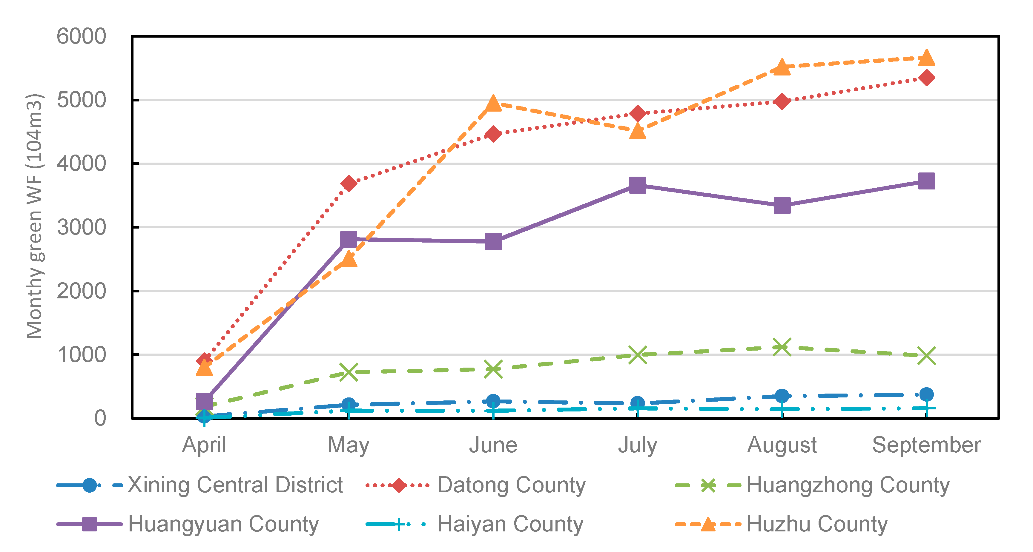
The green WF can affect the blue WF of the farming sector, which in turn has an impact on irrigation water requirements. According to the agricultural planting structure of the study area, there are three main types of crops: cereals (mainly wheat), canola, and vegetables, each with different growth cycle lengths. Crops are generally planted in April and harvested in September for one year, and the monthly green WF is accounted for in this period, due to the continental plateau climate characteristics of the study area.
Figure 5 shows the results of the monthly green WF of each region. The area of cultivated land in current and future scenarios is set to be consistent due to the relative stability of the farming sector. The annual green WFs of the six regions are quite different. The regions with larger planting areas (Datong County, Huangyuan County, and Huzhu County) are dozens of times larger than the other regions. In terms of the fluctuations in the monthly green WF, due to regional meteorological factors and crop growth cycles, there is a general upward trend from April to September. The green water footprint in the initial period is small and increases significantly during the rainy season (4–5 times). The spatial and temporal differences in the green WF are a significant representation of the irrigation water requirements in various regions.
3.1.2. Water Resource Demand Based on the Blue Water Footprint
Figure 6 (current scenario) and
Figure 7 (future scenario) show the results of the water resource demand based on the blue WF. As described in
Section 2.1.2, the water utilization of each region is divided into four sectors, including livelihood, farming, graziery, and industry. The farming sector accounted for a large proportion from April to September, which was even larger than 90% in Datong, Huzhu, and Huangyuan, which have more cropland. For the nonagricultural months (January–March and October–December), the proportions of the sectors in the different regions are quite different. Graziery had a relatively high proportion in Haiyan (68%) and Huangzhong (43%), while the livelihood sector in Xining Central District and Huzhu was higher. When compared with the farming sector, the water demand of the other sectors was not as noticeable and, thus, the farming sector determines the regional water resource demand.
Regarding temporal and spatial differences, the water demand of the different regions significantly varied with the seasons. During the nonagricultural months, the water demand in each region was relatively consistent; in April, May, and September (the seeding and harvesting periods, respectively), the differences among the regions began to increase and reached the maximum in summer (also the rainy season). The water demand of Datong and Huzhu were significantly higher than that of the other regions, which should be considered in the allocation of water resources. At the same time, all of the regions and the entire basin reached the peak water demand in summer.
For the future scenario, the water demand increased to some extent due to the increase in population and production. However, due to the small proportion of these sectors, the increase was mainly reflected in the nonagricultural months.
3.1.3. Pollutant Load Demand Based on the Grey Water Footprint
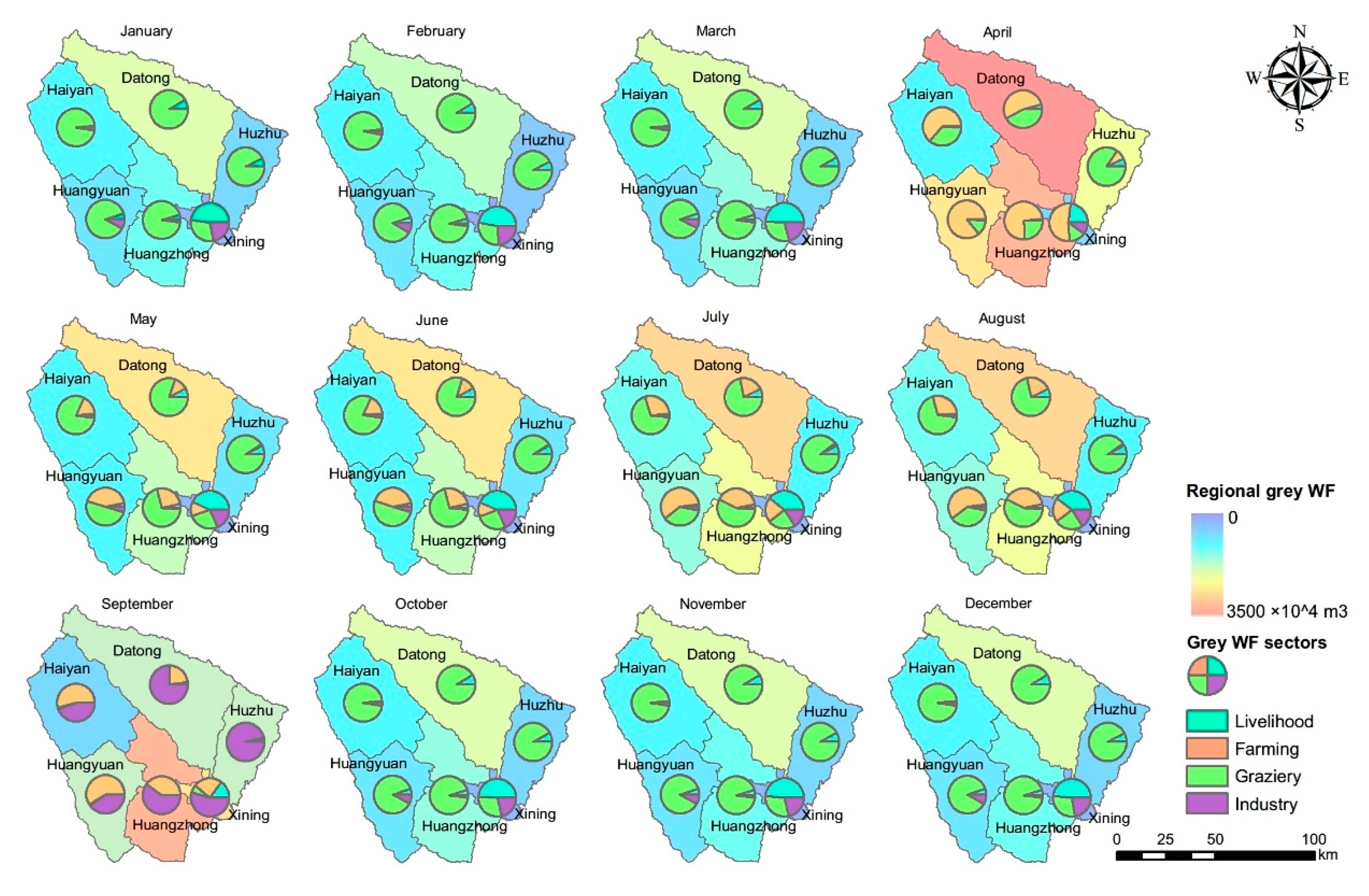
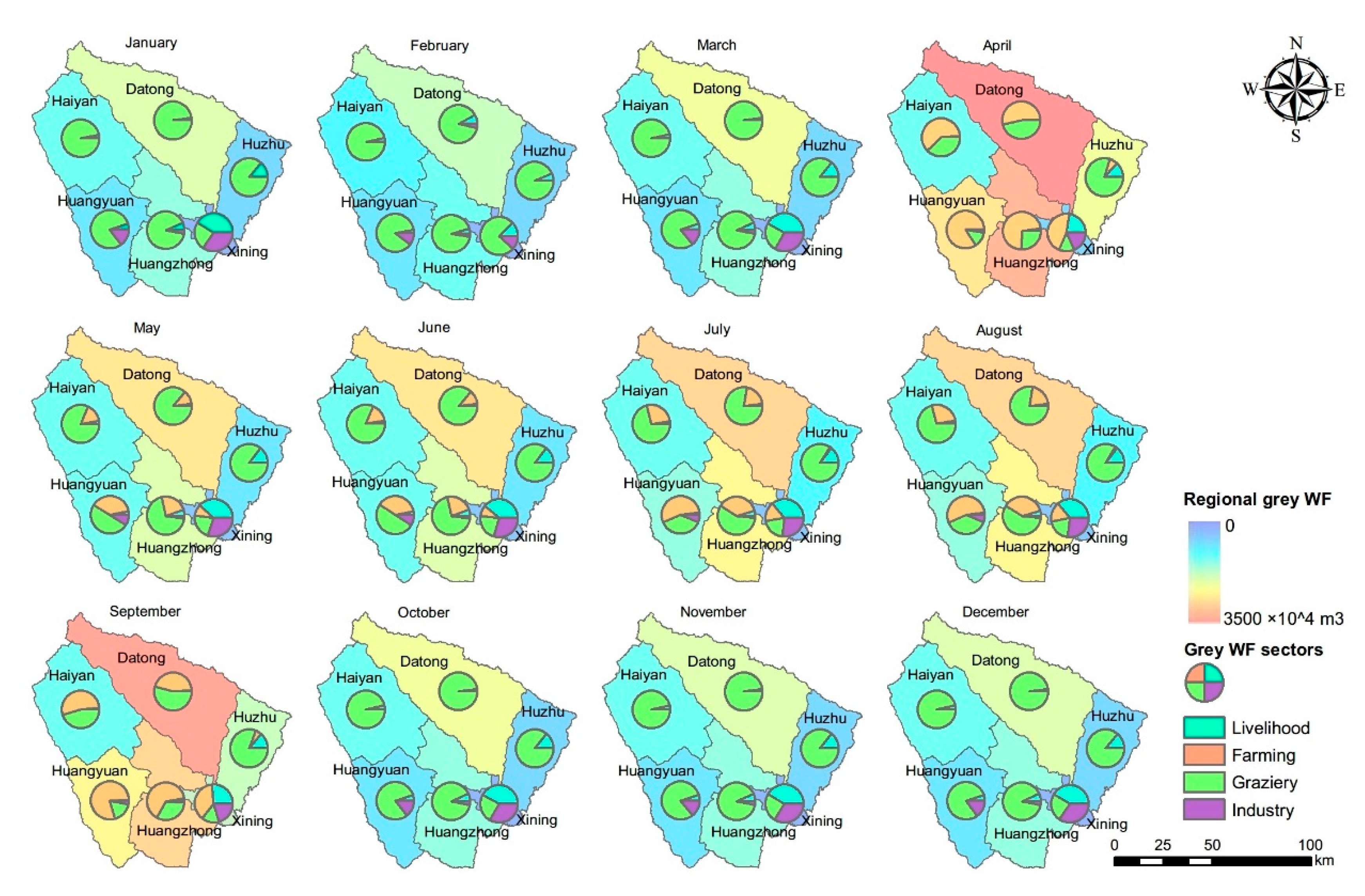
Figure 8 (current scenario) and
Figure 9 (future scenario) show the results of the pollutant load demand accounting based on the grey WF. When compared with the traditional pollution load expressed by physical quantity, the grey WF can consider the different environmental targets in each region and unify the pollution load into the same unit as the water resource.
The pollutant discharge structure of each region significantly changed with time, which was mainly related to the agricultural period. In the nonagricultural period, the dominant pollutant load was from graziery for most of the regions, while that of Xining Central District (with a higher urbanization level) was livelihood. During the beginning (April) and the end (September) of the agricultural period, a large amount of chemical fertilizers produced more nonpoint source pollution, and the proportion of farming began to increase, with Datong County and Huzhu County being the most significant.
Regarding temporal and spatial differences, the demand for sewage discharge in Datong County was the highest in most months, followed by Huangzhong County. The Xining Central District (located downstream of the basin) has the largest population and economy, and its pollutant load demand was low due to its higher sewage collection and treatment rate. The amount of pollutants in each region generally reached the highest level in spring and autumn, was moderate in summer, and lowest in winter.
For the future scenario, according to urban planning, the future industrial growth of Datong County is relatively large, and so is its increase in pollutant load discharge demand. The sewage discharge of the regions is still dominated by graziery, and the livelihood sector will discharge less with the increase in the urban sewage collection rate.
3.2. Initial Allocation Design Based on Bankruptcy Theory
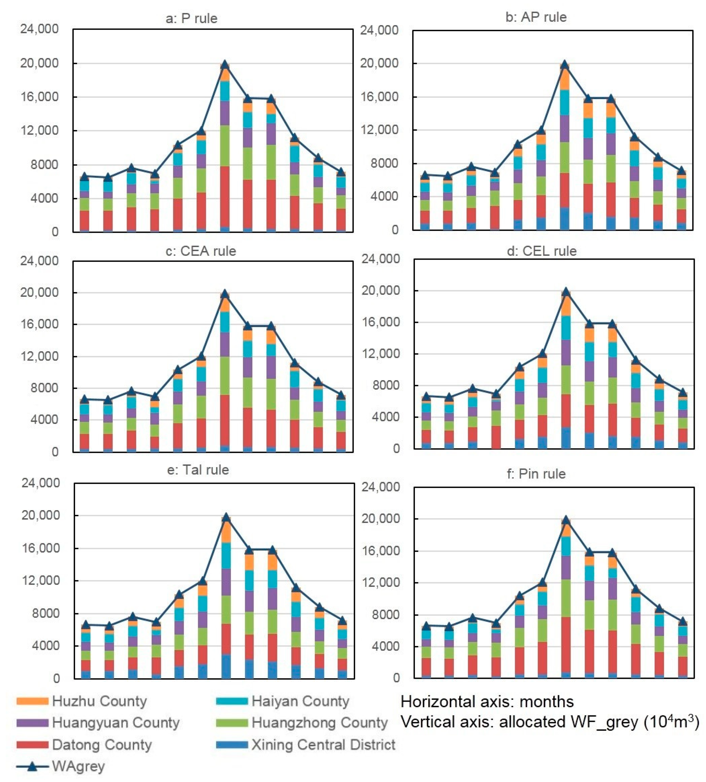
Figure 10 (blue WF) and
Figure 11 (grey WF) show the initial allocation schemes based on various bankruptcy rules in the current scenario. The results of the future scenario have larger scales and similar features and, thus, they are not shown here.
The polylines in
Figure 10 and
Figure 11 represent the allocable water resources and the environmental capacity based on the available water footprint, respectively. Clearly, the allocable resources are stably low in spring, rise to the peak of the year in summer (approximately twice), and gradually decrease in autumn. Based on the available WF accounting framework, the seasonal dynamic fluctuation can be accurately reflected.
Based on the six bankruptcy rules, the different initial allocation schemes have great distinctions, which are related to their respective allocation principles. As the simplest allocation rule, the
P rule is based on the proportion of the declarative requirements of various stakeholders. This allocation principle had a higher resource utilization efficiency for the whole basin, but its fairness is relatively weak and it objectively encourages the waste of resources. In the allocation scheme that is based on the
P rule (shown in
Figure 10a and
Figure 11a), the allocated resources of the different regions had large gaps. This problem has been somewhat relieved in the AP rule, as shown in
Figure 10b and
Figure 11b. The blue and grey water footprints were more evenly averaged across the regions throughout the year based on the AP rule.
The allocation principle of the CEA rule and the CEL rule are opposite: the former is conducive to stakeholders with less declarative demands, while the latter is conductive to stakeholders with larger demands. The results remarkably embody these characteristics. In the allocation scheme that is based on the CEA rule (
Figure 10c and
Figure 11c), Haiyan County and Xining Central District (with the lowest WF demand) are allocated a higher quantity when compared to that based on the other bankruptcy rules, while in the allocation results that are based on the CEL rule, due to the high demand for water resources in summer in Datong County and Huzhu County, the allocated quantity for the other regions is zero.
The Tal rule and the Pin rule are both comprehensive allocation approaches that combine the principles of the CEA and CEL rules, avoiding situations in which the stakeholders with higher or lower declarative requirements are excessively beneficial. When the allocable resource is relatively smaller as compared with the demand of the whole basin, their allocation schemes are the same, which is clearly reflected when the water resource demand is high in summer, as shown in
Figure 10e,f.
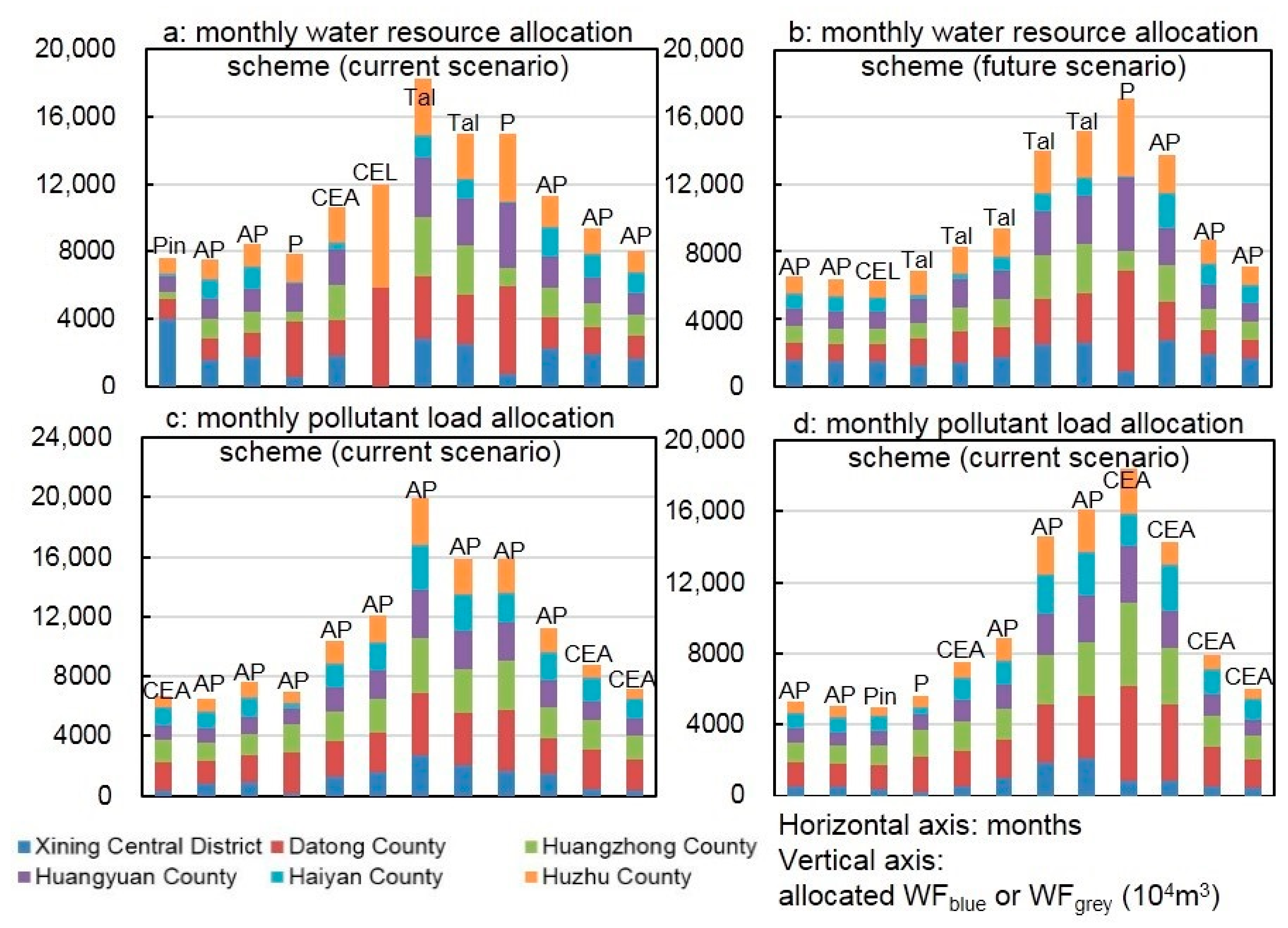
3.3. Allocation Optimization Based on Fallback Bargaining
After allocating the available blue WF and grey WF of each region in the basin based on various bankruptcy rules, the fallback bargaining (FB) approach was applied to optimize the initial allocation schemes.
For the goal of sustainable development, first, a WF sustainability assessment was conducted for each allocation scheme in the regions, and the preference ranking matrix was obtained based on the assessment results. Subsequently, the monthly optimal allocation schemes of the water resources (blue WF) and pollutant load (grey WF) could be obtained based on the fallback bargaining criteria that are described in
Section 2.4.2, as shown in
Figure 12.
Regarding water resource allocation, the FB approach chose different bankruptcy rules each month. For the allocated quantity of the various regions, the Xining Central District was adequately allocated in autumn and winter. In the summer, when the water resource demand of the farming sector surges intensely, the CEL rule and Tal rule were chosen as the allocation principles, guaranteeing the irrigation of Huzhu County and Datong County. The FB method can ensure the Pareto optimality of all the regional allocations in the basin [
53]. In addition, the monthly water resource demand that is based on blue WF accounting can pledge the efficient utilization of water resources and balance the seasonal changes in regional water use structures.
Regarding pollutant load allocation, the rules selected by FB were mainly the CEA rule and the AP rule. The CEA rule is conductive to regions with less pollutant discharge demand and it objectively encourages pollution reduction. According to the preference matrix that is based on grey WF sustainability, the water environmental quality of the region can be effectively guaranteed. In addition, the monthly allocation can make full use of the excess environmental capacity during the rainy season.
3.4. Applicability Analysis for the Allocation Framework
The purpose of this paper is to allocate water resource and discharge load while taking the development needs of different regions into account, in response to the shortage of water resource in the basin. However, for the basin with abundant resources that meet the need of development, the allocation scheme based on bankruptcy theory might not be suitable because of its “non-bankrupt” situation, which can only be regarded as a reference to the allocational approach. The six kinds of bankruptcy theory are discussed to explore their allocation patterns in the case of abundant resource ():
(1) For the
P rule, its allocation is based on the ratio of the declarative demand of each region. When
, according to Equation (13), the water resource and discharge load allocated to each region are greater than the declared demand, which does not match the sustainability target that is described in
Section 2.4.1.
(2) For the AP rule, the allocation amount is determined by the declarative demand of other regions and the total amount of resource in the basin (). When , the allocation amount of each region is calculated based on Equation (14), and the sum of them will be larger than . Therefore, the AP rule is not applicable to this case.
(3) For the CEA rule, according to Equation (15), when , the allocation amount of each region is equal to its declared demand. According to Equation (21), the sustainability index of all the regions (WSblue and WSgrey) are 1, so the CEA rule is the most optimal allocation mode.
(4) For the CEL rule, since this allocation mode is more advantageous for the regions that declare more demanding, the sum of the allocational amount for regions will be larger than according to Equation (16). Accordingly, the CEL rule does not meet the sustainability goals, similar to the AP rule.
(5) For the Tal rule, always meets the second condition of Equation (18) (), and the Tal rule will apply the CEL criterion. As shown in (4), the allocational amount of regions that are based on the Tal rule do not meet the sustainability goal.
(6) For the Pin rule, always meets the second condition of Equation (20) (), similarly to the Tal rule. Based on Equation (20), the allocational amount of each area is equal to that based on the CEA rule, so it is also a most optimal allocational mode.
In summary, when the water resource and environmental capacity in the basin are quite abundant, and the total resource () is larger than the sum of regional declaration demands (), the CEA rule and Pin rule are the most optimal allocation modes, and the P rule, the CEL rule, and the Tal rule are not sustainable. However, the AP rule is not suitable with this case.
4. Conclusions
This work proposed a monthly water resource and pollutant load allocation model for a basin that is based on the water footprint (WF) and fallback bargaining (FB). Unlike previous studies, the water resource and pollutant discharge demand are accounting for by the simulation of the anthropized water cycle, which not only reflects the monthly dynamics of water demand and sewage, but also considers the relationship between water quality and water volume. Several typical bankruptcy rules were applied to design various initial allocation schemes for water resources and pollutant loads after accounting for regional demands. Finally, with the goal of WF sustainability, the initial schemes were optimized by applying the FB approach. Overall, the monthly water resource and pollutant load allocation methodology framework can be summarized as four steps: (1) Monthly water use and pollutant discharge demand accounting-based WF; (2) Allocable resource accounting based on the available WF; (3) Initial allocation schemes designed based on bankruptcy rules; and, (4) Initial scheme optimization based on FB.
Regarding the case study, the Huangshui River basin is a typical seasonal and important irrigation area. There is a large area of cultivated land midstream, and the demand for water and sewage will sharply increase during the agricultural period; the regions downstream are the social and economic center of the entire basin, where the demographic and industrial scales are relatively large. Therefore, in different seasons, there are changeable contradictions of water resources and pollutant discharge among the regions upstream and downstream. WF accounting at the demand side can more accurately obtain the monthly dynamic changes in regional water utilization and pollutant discharge demand due to the comprehensive consideration of hydrology, meteorology, the crop growth cycle, the population, and the industrial water intensities in different seasons. The allocable resources are accounted for based on the available WF, while considering the ecological basic flue of the river. After accounting for the demand and allocable quantities, different bankruptcy rules were applied to design the initial allocation schemes. Some of the rules are conducive to regions with a higher declarative demand, while others are conductive to regions with lower demand. Finally, with the goal of WF sustainability, the FB method was applied to optimize the initial schemes, ensuring that the preferred scheme achieves agreement for each region. In the final allocation results, different bankruptcy rules were adopted in different months. In terms of water resource allocation, under the premise of satisfying the water demand of the Xining Central District downstream, more water resources were allocated to Datong County and Huzhu County in summer to ensure irrigation. The bankruptcy rules that were applied in the monthly pollutant load allocation mainly included the AP and CEA rules, which can encourage high pollutant regions to reduce emissions.


