Carbon Sequestration Total Factor Productivity Growth and Decomposition: A Case of the Yangtze River Economic Belt of China

Abstract

To find out whether carbon sequestration is both effective at mitigating climate change and promoting economic growth, in this paper, by adopting a stochastic frontier panel model with translog production function, carbon sequestration is incorporated into endogenous variables to establish estimation model of carbon sequestration total factor productivity (CSTFP) and examine CSTFP growth and its drivers decomposition of the Yangtze River Economic Belt (YREB) of China in three estimations. The result shows that, (1) compared to traditional TFP growth, CSTFP growth in YREB is improved by 26.74 percentages (from −26.55% to 0.20%), contributed by three positive drivers of technical efficiency change (28.59%), technological progress change (18.55%), and scale efficiency change (3.99%); (2) different CSTFP growth exists in three watershed segments of YREB, which firstly is the upper reaches (0.62%), then the lower reaches (0.11%) and the middle reaches (−0.14%). Improved CSTFP growth owes to carbon sequestration’s harmonious symbiosis where natural ecosystems and human activities are naturally blended while insufficient synergies are bottleneck for promotion of CSTFP growth in YREB. Related policy suggestions are provided in the end. The proposed analysis framework is efficient to disclose CSTFP growth in YREB, and can also be applied to similar analysis on CSTFP in regions and extended to multi-country/region analysis.

1. Introduction

Facing challenges of global climate change, carbon sequestration can endogenously drive both economic development and mitigate climate change. CO₂ emissions reduction and carbon sequestration are both effective measures for dealing with dilemmas between promoting economic development and mitigating climate change [1,2]. Compared to CO₂ emissions reduction in reality, carbon sequestration can fundamentally promote win-win strategy of economic development and mitigate climate change by two ways. One is carbon sinks and reservoirs of CO₂ through photosynthesis, such activities as sustainable forest management practices, afforestation and reforestation, and sustainable forms of agriculture [2]. Because, photosynthesis can make the plant convert CO₂ and water into organic material and release oxygen through biochemical process under visible light irradiation, with light and dark reaction and the use of photosynthetic pigment. As the basis of the biosphere’s survival, photosynthesis is the main driver of the global carbon cycle, closely linked to the climate system through numerous feedback processes [3,4], which are associated with extreme weather events, such as heat waves, droughts, and floods [5,6]. More importantly, photosynthesis can increase crop yields and plant products production for the needs of population and economic growth [7,8]. The other way is artificial carbon capture and use through activities of technical innovation and clean development, such as enhancement of energy efficiency in relevant sectors of the national economy, new and renewable forms of energy, research and development (R&D), and increased use of CO₂ sequestration technologies and of advanced and innovative environmentally sound technologies [2].

Carbon sequestration is efficient for improvement of productivity growth. On the aspect of natural reproduction, carbon sequestration creates gross primary production, the absorption of atmospheric CO₂ by plants through photosynthesis, raises ecosystem productivity and contributes to mitigating global warming [9,10]. On the aspect of human activity, carbon sequestration stimulates human productivity and increases output value by offering abundant natural resources for human production activity and economic development. Forest carbon sinks, for example, promote efficiency of ecological economy and green total factor productivity of forests by supply of forest coverage, fresh air, green environment and wood, medicine, mushrooms, and other human production and living necessities [1,11,12]. Especially under the challenge of the green paradox where carbon tax or subsidies to carbon capture, use and storage (CCUS) technology cause higher global emissions through stimulating fossil fuel production [13,14,15], to disclose the endogenous characteristics of carbon sequestration to total factor productivity (TFP) growth and its driver decomposition is extremely inevitable and valuable for sustainable economic development and environmental conservation.

Carbon sequestration as an endogenous variable to TFP growth is in need of urgent discussion. For research of source of productivity growth, scholars used classical production function of the Solow residuals to explore TFP growth by introducing capital, labor, and gross domestic product (GDP) into consideration [16,17,18,19,20]. In the face of increasingly environmental problems caused by CO₂ emissions, regarding CO₂ emissions as negative residual output, together with positive output such as GDP, some researchers took energy consumption and environmental impacts such as CO₂ emissions as endogenous variables into the production function, constructed estimation model to examine green TFP growth [21,22,23,24,25,26,27,28,29,30,31,32,33,34,35]. Basically, two lines of researches on green TFP growth exist in literature. One line is mainly focused on estimating the industrial green TFP growth of fossil energy-intensive industries and sectors, such as estimation of green TFP of Swedish and Canadian pulp and paper industries [21], investigation of green TFP of China’s industrial sectors [22,23,24,25,26,27,28], and measurement of ecological economic efficiency and TFP of forests in China [1]. The other line is focused on green TFP growth at the national or regional level. Examples are the exploration on environmentally sensitive productivity growth of 41 developing and developed countries [29], green and environmental TFP measure of China’s provinces and regional economies [30,31,32,33], the drivers of TFP change with an illustrative example of 14 EU countries [34], and aggregate green productivity growth estimation at the aggregate level in countries from the Organization for Economic Co-operation and Development (OECD) [35]. Carbon sequestration’s endogenous feature to TFP growth is ignored, although a few scholars discussed the functions of forest carbon sinks on TFP of forest and economic growth [1,11,36], however, at the aggregate level, carbon sequestration is not introduced as an impact factor to measure the TFP growth in the literature; and again, most studies on TFP are based on perspective of administrative area, without consideration of watershed geographic correlations of TFP growth in natural river basin regions.

Since carbon sequestration is effective for dealing with dilemmas between economic growth and environmental protection both by carbon sinks and reservoirs of CO₂ through photosynthesis and by artificial carbon capture and use through activities of technical innovation and clean development, it is of great necessity to discuss the role of carbon sequestration as an endogenous variable of TFP growth especially in natural river basin regions by estimation of carbon sequestration total factor growth (CSTFP) growth.

For assessment of the CSTFP growth, the stochastic frontier analysis (SFA) is adoptable. Up to now, abundant literature has sought various approaches to open the “black box” of the TFP growth; the stochastic frontier analysis (SFA) is one of the main approaches in the application of estimating TFP growth. SFA was originally proposed by Aigner et al. and Meeusen and van den Broeck [37,38], and has been broadly applied by many researchers into study [39,40,41,42,43,44,45,46,47,48,49,50,51,52,53,54] due to the following fundamental advantages. Firstly, it can explain more accurately the theoretical definition of a production function which estimates the maximum output attainable from a given set of inputs, and secondly, the technical efficiency of the sample may be estimated by comparing the observed output with the predicted (or attainable) output [44,46,55,56,57]. Thus, SFA is appropriate for the investigation of CSTFP growth.

Drivers decomposition of CSTFP growth needs consideration on integration of technology progress, technical efficiency change, factor allocation efficiency change, and scale efficiency change. On the drivers of TFP growth, technical effect and technology progress at the national level are discussed but the structural effect and scale effect at the regional level are ignored in most literature [58,59,60,61,62,63,64,65,66]. Actually, even if all regions are efficient, it is still required to optimize resource utilization for the TFP growth at the regional level through coordination for improvement of input–output mixes [67]. Recognizing the shortage of previous research, some scholars have tried to improve analysis on the structural effect or/and scale effect in decomposition of TFP growth [68,69,70,71], such as a decomposition of TFP indicator into components of technical change, technical inefficiency change, and scale inefficiency change on the agricultural sector at the state-level in the U.S. [68] and measurement of green productivity evolution for 30 OECD countries with decomposition for green productivity growth changes into technological progress, technical efficiency change, and structural efficiency change [35]. But, integration of technology progress, technical efficiency change, factor allocation efficiency change, and scale efficiency change has yet to be discussed in literature. Considering carbon sequestration’s harmonious symbiosis where natural ecosystems and human activities are naturally blended in the same regions, drivers decomposition of CSTFP growth requires examination on the base of integration of technology progress, technical efficiency change, factor allocation efficiency change, and scale efficiency change.

Based on the above research findings and shortcomings, this paper adopts the stochastic frontier approach with translog production function to estimate the CSTFP growth and discusses its drivers decomposition with the case study of the Yangtze River Economic Belt (YREB) of China. The main innovative contributions to the literature is as follows.

First, although some scholars investigated TFP growth by introducing energy consumption, carbon emissions, and other variables in the production functions, or discussed the interaction between forest carbon sinks and economic growth, there still lacks an analysis on the impact of carbon sequestration on TFP growth. In this paper, carbon sequestration as an endogenous variable is introduced into the production function to investigate CSTFP growth from the perspective of input–output mixes and discloses its impact on TFP growth by comparison of results in three estimations.

Second, most literature focus on analysis of the industrial TFP or regional TFP growth from the level of administrative areas but neglect the watershed geographic correlations of TFP growth in the same river basin. In this paper, the focus on carbon sequestration’s characteristics of collaborative symbiosis between economic development and environment optimization, the difference of CSTFP growth with different watershed characteristics of the same river basin, are disclosed.

Third, decomposition of TFP growth in the current research is analyzed by only the use of three components of technical progress, technical efficiency change and scale efficiency change, or those of technical progress, technical efficiency change, and factor allocation efficiency change. By decomposition of CSTFP growth in this paper, four components of technical progress, technical efficiency change and scale efficiency change and factor allocation efficiency change are integrated together to disclose the drivers of CSTFP growth and their harmonious coexistence in YREB.

The structure of this paper is as follows. In Section 2, the conceptual framework and model are presented. Section 3 presents the study area and data, Section 4 is empirical estimation, Section 5 delivers results, and Section 6 is the discussion. Section 7 is the conclusion with policy implications.

2. Methodology

2.1. Conceptual Framework

As Figure 1 shows, the conceptual framework of CSTFP growth estimation is set up based on features caused by carbon sequestration’s harmonious symbiosis correlations between economic development and environment optimization as follows.

Firstly, compared to CO₂ emissions as undesirable output, carbon sequestration is desirable output which produces watershed harmonious symbiosis where natural ecosystems and human activity circle are naturally blended in economic regions. On the environmental sphere, carbon sequestration creates gross primary production, the absorption and decomposition of atmospheric CO₂ by plants through photosynthesis, raises ecosystem productivity, and contributes to mitigating global warming in natural ecosystem of economic regions [9,10]. On the economic sphere, carbon sequestration promotes human productivity and makes output value added by offering abundant natural resources for human activities of production and life in the human activity circle of economic regions [1,11,36].

Secondly, as an endogenous variable with integration of other relative variables such as labor, capital, energy consumption, CO₂ emissions, industrial structure, open-up, R&D, and urbanization, carbon sequestration’s synergy effect on CSTFP growth is showed from the perspective of input–output mixes. On the end of input, carbon sequestration stimulates factor investment such as labor, capital, and technology into primary productive activities of afforestation, agriculture, forestry, and ecological restoration of rivers, grasslands, and wetlands, as well as human productive activities of manufacturing and services, resulting in the superposition of relevant elements of input. On the end of output, carbon sequestration makes CO₂ absorbed through photosynthesis of nature to release oxygen or clean production to capture and use CO₂, providing diversified products such as timber, food, and other raw materials for the human society, promoting integration of natural reproduction and social reproduction synchronously.

Thirdly, focus on the target of green and low-carbon sustainable growth of economic regions, the growth of CSTFP is estimated by the stochastic frontier panel model with translog production function with introduction of relative core variables and exogenous variables, and the four drivers of technical progress, technical efficiency change, scale efficiency change, and factor allocation efficiency change are integrated to drive the CSTFP growth for the sustainable development of economic growth and environmental conservation. Thus, is disclosed that the growth of CSTFP and its four-driver linkage naturally promote the harmonious co-prosperity of the human activity circle and natural ecosystem in economic regions.

Based on the conceptual framework of CSTFP growth estimation, the relative methodology is discussed in detail as follows.

2.2. Stochastic Frontier Analysis

For estimating CSTFP growth in YREB, stochastic frontier analysis (SFA) is introduced in this paper. Actually, SFA is originally used to study production optimization [37,38,39]. The models of SFA adopt the compound residual measure, and can simply be expressed as follows:

$${\mathrm{y}}_{it}=f[x_{it}(t),\beta ]\times \exp (v_{it}-{\mu }_{it}),{\mu }_{it}\ge 0$$

(1)

$$v_{it}\approx N(0,{\sigma }_{\mathrm{v}}^2)$$

(2)

$${\mu }_{\mathrm{it}}\approx N^{+}({\mu }_{it},{\sigma }_{\mathrm{it}}^2)$$

(3)

$${\mu }_{it}=z_{it}\delta$$

(4)

$${\sigma }_{\mathrm{it}}^2=\exp (z_{it}\theta )$$

(5)

$${\sigma }_v=\exp (z_{it}\lambda )$$

(6)

where Equation (1) is stochastic frontier production function; i means the provincial region, i = 1, 2, …, n. t means time, t = 1, 2, …, n; $y_{it}$ is Logarithm of actual local gross domestic product for province i in period t; $f[X_{it}(t),\beta ]$ is Frontier production function; $X_{it}(t)$ is Production factor combination; $\beta$ is Coefficient to be estimated; $({\upsilon }_{it}-{\mu }_{it})$ is Compound error structure, supposed ${\mu }_{\mathrm{it}}$ and ${\upsilon }_{\mathrm{it}}$ is independent, and it is assumed that these two kinds of errors are not related to $X_{it}(t)$; if $({\upsilon }_{it}-{\mu }_{it})>0$, the sum of noise effect and technical efficiency is positive, indicating that the output is above the determined value of production frontier. Conversely, below the determined value of production frontier. ${\upsilon }_{\mathrm{it}}$ is random error terms assumed to be independent and identical distribution.

Equation (2) shows that the distribution of random error term ${\mu }_{\mathrm{it}}$ follows a semi-normal distribution and is a non-negative random variable. Equation (3) indicates the distribution of the technical invalidity rate term. Equation (4) is the mean value equation of technical inefficiency. $z_{it}$ is a set of exogenous explanatory variables affecting technological inefficiency. $\delta$ is coefficient of explanatory variable of the technical inefficiency equation. If coefficient is positive, the variable has a positive effect on the inefficiency term. Equation (5) is technical invalidity rate term variance equation, $\theta$ is the value to be estimated of the coefficient of variance of technical inefficiency term. Equation (6) is stochastic error term variance equation, $\lambda$ is the value to be estimated of the coefficient of variance of random error term.

Where ${\sigma }^2={\sigma }_{\upsilon }^2+{\sigma }_{\mu }^2$ represents the variance of the compound residual term which is $({\upsilon }_{it}-{\mu }_{it})$. Battese [42,43] set variance parameter as $\gamma ={\sigma }_{\mu }^2/{\sigma }^2(\gamma \in [0.1])$ in order to verify the reasonableness of adopting SFA. If $\gamma$ is close to 1, it is reasonable and necessary to adopt SFA model. If $\gamma$ is close to 0, the least square estimation can be used.

2.3. Translog Production Function Setting

When constructing the SFA model to measure the CSTFP growth, the appropriate approach will be used to test it. Meanwhile, the production function should be satisfied with conditions that any one of the four input variables as labor input (L), capital input (K), energy consumption (E), and carbon sequestration (CS) is affected by the other three input variables, as well as the formation of scale effect and factor allocation effect. Compared with the Cobb–Douglas production model, Leontief’s production model and the constant elastic production model, translog production function not only eliminate substitution effect and interaction between input elements, but also reflect influence of time variation, so it is more general [37,38,39,40,41,42,43,44,45,46]. The errors caused by the function can be effectively avoided [37,38,39,40,41,42]. Therefore, translog production function with time variable as specific form of the frontier production function is adopted in this paper, that is:

$$\begin{array}{l}\ln y_{it}=\ln f[X_{it}(t),\beta ]+({\upsilon }_{it}-{\mu }_{it})\\ ={\beta }_0+{\beta }_1\ln L_{it}+{\beta }_k\ln K_{it}+{\beta }_e\ln E_{it}+{\beta }_{cs}\ln C{S}_{it}+{\beta }_{l}t+{\beta }_{l^2}(\ln L_{it}{)}^2\\ +{\beta }_{k^2}(\ln K_{it}{)}^2+{\beta }_{e^2}(\ln E_{it}{)}^2+{\beta }_{c{s}^2}(\ln C{S}_{it}{)}^2+{\beta }_{l^2}{t}^2+{\beta }_{lk}\ln L_{it}\ln K_{it}\\ +{\beta }_{le}\ln L_{it}\ln E_{it}+{\beta }_{ke}\ln K_{it}\ln E_{it}+{\beta }_{lcs}\ln L_{it}\ln C{S}_{it}+{\beta }_{kcs}\ln K_{it}\ln C{S}_{it}\\ +{\beta }_{ecs}\ln E_{it}\ln C{S}_{it}+{\beta }_{lt}t\ln L_{it}+{\beta }_{kt}t\ln K_{it}+{\beta }_{et}t\ln E_{it}+{\beta }_{cst}t\ln C{S}_{it}\end{array}$$

(7)

2.4. Technical Inefficiency Function Setting

For the purpose of investigating influence of factors of second industry ratio of (CI) to (SI), urbanization rate (UE), R&D (RD), opening outside (OP) on CSTFP growth, the mean value equation of technical inefficiency is introduced on the basis of (7) as the following [42,43]:

$${\mu }_{it}={\delta }_0+{\delta }_{1}C{I}_{it}+{\delta }_{2}S{I}_{it}+{\delta }_{3}U{E}_{it}+{\delta }_{4}R{D}_{it}+{\delta }_{5}O{P}_{it}$$

(8)

where ${\mu }_{it}$ is a random error term.

2.5. Decomposition of CSTFP Growth

Based on the relative analysis on TFP decomposition [46,56,57], in this paper, the growth rate of CSTFP can be decomposed into four components: technical progress (ΔTP), technical efficiency change (ΔTE), scale efficiency change (ΔSE), and factor allocation efficiency change (ΔAE).

2.5.1. Rate of Technical Progress

The rate of technological progress refers to the change rate of output varying over time with that the relevant input is constant. It shows moving up or down of the production frontier curve along with change of frontier technological progress, as follows [46,56,57]:

$$∆TP=\frac{\partial \ln f[X_{it}(t),\beta ]}{\partial t}={\beta }_t+2{\beta }_{r^2}t+{\beta }_{lt}\ln L_{it}+{\beta }_{kt}\ln K_{it}+{\beta }_{et}\ln E_{it}+{\beta }_{cst}\ln C{S}_{it}$$

(9)

2.5.2. Rate of Technical Efficiency Change

It is the change rate of the ratio of actual output to frontier output with time under premise that the cutting-edge technology level is constant, and that of actual output to frontier output with given factors input. It reflects the change in proportion of output over time that the actual efficiency of cutting-edge technology has failed to reach. It measures capacity of producers to use technology, as follows [46,56,57]:

$$∆TE=\frac{d\ln \left\{\frac{f[X_{it}(t),\beta ]\times \exp ({\upsilon }_{it}-{\mu }_{it})}{f[X_{it}(t),\beta ]\times \exp ({\upsilon }_{it})}\right\}}{dt}=-\frac{d\stackrel{\wedge }{{\mu }_{it}}}{dt}$$

(10)

2.5.3. Rate of Scale Efficiency Change

It refers to the change of output corresponding to the increase of factor input with expansion of production scale, which can be in three situations: increasing rate, decreasing rate, and keeping it constant, as follows [46,56,57]:

$$\begin{array}{l}∆SE=(\epsilon -1){\displaystyle {\displaystyle \sum }_j}\frac{{\epsilon }_j}{\epsilon }\times \stackrel{.}{x_j}\\ =({\epsilon }_l+{\epsilon }_k+{\epsilon }_e+{\epsilon }_{CS}-1)\times \left(\begin{array}{l}\frac{{\epsilon }_l}{{\epsilon }_l+{\epsilon }_k+{\epsilon }_e+{\epsilon }_{cs}}\times \frac{∆L}{L}+\frac{{\epsilon }_k}{{\epsilon }_l+{\epsilon }_k+{\epsilon }_e+{\epsilon }_{cs}}\times \frac{∆K}{K}\\ +\frac{{\epsilon }_e}{{\epsilon }_l+{\epsilon }_k+{\epsilon }_e+{\epsilon }_{cs}}\times \frac{∆E}{E}+\frac{{\epsilon }_{cs}}{{\epsilon }_l+{\epsilon }_k+{\epsilon }_e+{\epsilon }_{cs}}\times \frac{∆CS}{CS}\end{array}\right)\end{array}$$

(11)

where ${\epsilon }_j(j=l,k,e,cs)$ represents separately output elasticity of labor, capital, energy consumption, or carbon sequestration; $\epsilon$ is the overall factor scale elasticity, which is the sum of output elasticity of labor, capital, energy consumption, and carbon sequestration. If $\epsilon =1$, this part obviously does not have to be added; if $\epsilon \ne 1$, when the scale efficiency ratio is more than 1, the increase rate of productivity will be raised by increasing the input quantity of factors. But if the scale efficiency is less than 1, the scale of output can only be reduced. $\stackrel{.}{{\displaystyle x_j}}$ is the change rate of factor input:

$${\epsilon }_l=\frac{\partial \ln y}{\partial \ln L}={\beta }_l+2{\beta }_{l^2}\ln L_{it}+{\beta }_{lk}\ln K_{it}+{\beta }_{le}\ln E_{it}+{\beta }_{lcs}\ln C{S}_{it}+{\beta }_{lt}t$$

(12)

$${\epsilon }_k=\frac{\partial \ln y}{\partial \ln K}={\beta }_k+2{\beta }_{k^2}\ln K_{it}+{\beta }_{lk}\ln L_{it}+{\beta }_{ke}\ln E_{it}+{\beta }_{kcs}\ln C{S}_{it}+{\beta }_{kt}t$$

(13)

$${\epsilon }_e=\frac{\partial \ln y}{\partial \ln E}={\beta }_e+2{\beta }_{e^2}\ln E_{it}+{\beta }_{le}\ln L_{it}+{\beta }_{ke}\ln K_{it}+{\beta }_{ecs}\ln C{S}_{it}+{\beta }_{et}t$$

(14)

$${\epsilon }_{cs}=\frac{\partial \ln y}{\partial \ln CS}={\beta }_{cs}+2{\beta }_{c{s}^2}\ln C{S}_{it}+{\beta }_{lcs}\ln L_{it}+{\beta }_{kcs}\ln K_{it}+{\beta }_{ecs}\ln E_{it}+{\beta }_{cst}t$$

(15)

2.5.4. Rate of Factor Allocation Efficiency Change

The rate of factor allocation efficiency change mainly examines the contribution of structural change of factor allocation to CSTFP growth in the process of production with given frontier technology level, as follows [46,56,57]:

$$\begin{array}{l}∆AE={\displaystyle \sum _j}[(\frac{E_j}{E}-s_j)]\times \stackrel{.}{{\displaystyle x_j}}\\ =\left(\frac{{\epsilon }_l}{{\epsilon }_l+{\epsilon }_k+{\epsilon }_e+{\epsilon }_{cs}}-\frac{L_t}{L_t+K_t+E_t+C{S}_t}\right)\times \frac{∆L}{L}+\left(\frac{{\epsilon }_k}{{\epsilon }_l+{\epsilon }_k+{\epsilon }_e+{\epsilon }_{cs}}-\frac{K_t}{L_t+K_t+E_t+C{S}_t}\right)\times \frac{∆K}{K}\\ +\left(\frac{{\epsilon }_e}{{\epsilon }_l+{\epsilon }_k+{\epsilon }_e+{\epsilon }_{\mathrm{cs}}}-\frac{E_t}{L_t+K_t+E_t+C{S}_t}\right)\times \frac{∆E}{E}+\left(\frac{{\epsilon }_{cs}}{{\epsilon }_l+{\epsilon }_k+{\epsilon }_e+{\epsilon }_{cs}}-\frac{C{S}_t}{L_t+K+E_t+C{S}_t}\right)\times \frac{∆CS}{CS}\end{array}$$

(16)

where $s_j$ represents the proportion of a certain factor per unit cost, $\frac{E_j}{E}-s_j$ means there is difference between the ratio of output elasticity of a certain factor to unit cost and that of unit cost. When the value is positive, it shows the factor allocation efficiency has been improved, and conversely, the factor allocation efficiency has been worsened.

On the basis of the methodology discussed above, next, let us come to the study area of YREB and related data analysis.

3. Study Area and Data

3.1. The Yangtze River Economic Belt (YREB) of China

As Figure 2 shows, the YREB is an economic belt with watershed features of harmonious symbiosis where natural ecosystems and human activities are naturally blended. It spans the diversified topography of the western high mountains, the central hilly valley, and the eastern plain delta, it belongs to the subtropical and warm temperate climatic belt and the intersection of the southeast ocean warm current and the northwest plateau cold current with four distinct seasons and rainfall. It is abundant with lush forests, diversified agriculture, modern manufacturing, and a prosperous economy. It is a bridge linked with China’s eastern coastal leading economic zone, the western great developing zone, and the central rising economic zone.

The YREB covers 9 provinces of Sichuan, Yunnan, Guizhou, Hubei, Hunan, Jiangxi, Anhui, Jiangsu, and Zhejiang and 2 municipalities of Chongqing and Shanghai. For the sake of comparative analysis, it is divided into three watershed segments: the upper reaches, the middle reaches, and the lower reaches (Yangtze River Delta). The upper reaches include 3 provinces and 1 municipality of Sichuan, Guizhou, Yunnan, and Chongqing; the middle reaches include 4 provinces of Anhui, Jiangxi, Hunan, and Hubei; and the lower reaches include 2 provinces and 1 municipality of Zhejiang, Jiangsu, and Shanghai.

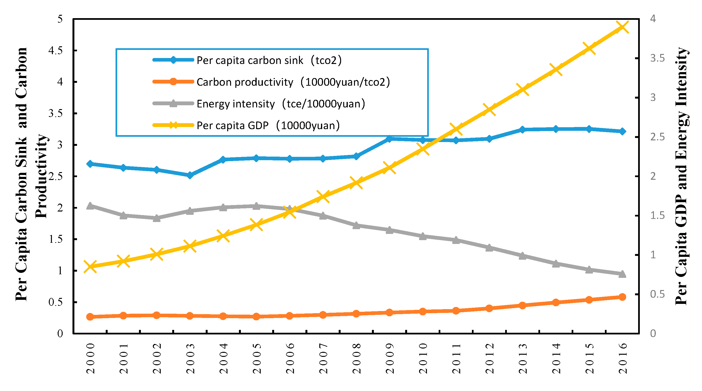
Recently, the YREB is the biggest natural river basin economic belt, accounting for 40% of China’s population and GDP as well as CO₂ emissions. Since 2000, as shown in Figure 3, carbon sequestration and carbon productivity have increased while energy intensity decreased, along with growth of GDP per capita, economic development correlates ever closer with energy consumption and carbon sequestration. So, it is very valuable to investigate the CSTFP growth in the natural river basin economic belt of YREB.

3.2. Variables and Data

In this paper, the growth of CSTFP in YREB is measured based on data of 2000–2016 from statistical yearbooks of 11 provinces and municipalities of the YREB [72,73]. For meeting the needs of analysis on CSTFP growth and decomposition as in Figure 1, the total variables and data are firstly discussed as the following. The regional actual GDP is used as the index of output variable, the labor (L), capital (K), energy consumption (E), and carbon sequestration (CS) are taken as input variables; and the carbon emission intensity of (CI), the second industry ratio (SI), urbanization rate (UE), R&D level (RD), and open-door level (OP) are the explanatory variables of technical inefficiency. The statistical description of the variables selected in this paper is shown in

Table 1. Descriptive statistics of key variables [72,73].

	Variables	Marks	Observed Values	Mean	S.D.	Min.	Max.
Explained variable	Local GDP (RMB 100 million yuan)	Y	187	11,056.22	9438.172	993.53	53,138.6
Explanatory variable	Labor (10,000 workers)	L	187	3058.321	1201.332	752.26	4860
	Capital stock (RMB 100 million yuan)	K	187	22,509.77	20,796.25	1776.29	119,790
	Energy consumption (10,000 ton)	E	187	10,154.21	5792.988	2331.52	32,876.9
	carbon sequestration (10,000 ton)	CS	187	15,686.54	8962.507	501.5	34,729.8
Exogenous variables	Carbon emission intensity (ton/10,000RMB¥)	CI	187	0.8894	0.5141	0.3316	3.1028
	Ratio of secondary industry (%)	SI	187	46.04	5.3618	29.83	56.6
	Urbanization rate (%)	UE	187	47.51	15.77	23.36	89.6
	Research and development level (%)	RD	187	1.2817	0.7167	0.3478	3.726
	Opening level (%)	OP	187	30.4	38.4908	3.3477	158.333

Note: Considering that the exchange rate of RMB yuan to US dollar is changeable (for example, the currency in early January of year 2000 was 8.27 RMB¥ to 1 US$ and in December of year 2015 reached 6.45 RMB¥ to 1 US$. During the period 2000–2016, the min and max values fluctuated from 6.33 to 8.2797) [72,73], here we take RMB¥ as the unit of value in data processing.

.

3.2.1. Output and Input Variables

(1) Total output variable (unit: 100 million RMB¥). GDP is selected as total output of each province in YREB. The nominal GDP is converted into real GDP on the base of consumer price index of the year 2000. As total output variable, GDP is recorded as Y.

(2) Labor input variables (unit: 10,000 people). The year-end number of employees is selected as labor input of each province in YREB, and is recorded as L. The nominal average salary data of employees is converted into real average salary data based on consumer price index of the year 2000 as cost of labor input.

(3) Capital stock input variables (unit: 100 million RMB¥). The method of perpetual storage is used here that the formula is $K_{it}=I_{it}/P_{it}+K_{it-1}(1-\rho )$, $I_{it}$ represents total fixed capital formation, $P_{it}$ is fixed asset formation price index, $\rho$ is fixed assets depreciation rate (here is 10.96%) [74]. The formula for calculating the initial capital stock is $K_{it}=I_{it}/(g_{it}+\rho )$, among which, $g_{it}$ is mean value of the growth rate of the total fixed capital formation in the provinces and municipalities from 2000 to 2004. Through the above methods to obtain the real stock of capital in each province, is recorded as K.

(4) Energy input variables (unit: 10,000 tons of equivalent coal). In research of this paper, data on energy consumption and fossil energy equivalent coal coefficient from 2000 to 2016 was obtained from China Statistical Yearbooks and China Energy Statistical Yearbooks. Using annual energy consumption of each province as energy input, the consumption of coal, coke, crude oil, gasoline, kerosene, diesel, fuel oil, natural gas, and other energy is converted into a unified unit due to their different categories of energy consumption in each province. “Tonnes of equivalent coal” (see

Table 2. Equivalent coal converted coefficient of fossil energy and carbon emissions factor [75].

Indexes	Equivalent Coal Factors	Carbon Emission Factors
Raw coal	0.7143	0.7559
Coke	0.9714	0.855
Crude oil	1.4286	0.5857
Petrol	1.4714	0.5538
Kerosene	1.4714	0.5714
Diesel oil	1.4571	0.5921
Fuel oil	1.4286	0.6185
Nature gas	1.33	0.4483
Coke oven gas	0.5928	0.3548

), the total energy consumption is recorded as E. The nominal unit price of equivalent coal, coming from the nationally announced coal-fired power generation grid benchmark price, is converted into real unit price of equivalent coal on the base of consumer price index of the year 2000. In 2016, the coal-fired power generation benchmark price is derived from the website of China National Development and Reform Commission.

(5) Carbon sequestration input variables (unit: 10,000 tons of carbon dioxide). Carbon sequestration mainly refers to the amount of carbon dioxide absorbed and stored by nature such as forest vegetation, agricultural crops, wetlands, and offshore water. The factors and indicators of carbon sequestration are shown in

Table 3. Carbon sequestration conversion coefficient.

Categories	Factor	Unit
Forest [76]	13.97	tCO2/hm2
Artificial wetland [77,78]	6.07	tCO2/hm2
Inshore and coastal [77,78]	3.70	tCO2/hm2
River [77,78]	2.19	tCO2/hm2
Lake [77,78]	1.47	tCO2/hm2
Rice [79]	3.50	tCO2/t
Wheat [79]	2.66	tCO2/t
Corn [79]	2.71	tCO2/t
Beans [79]	2.48	tCO2/t
Potatoes [79]	1.71	tCO2/t
Peanut [79]	3.15	tCO2/t
Rapeseed [79]	1.83	tCO2/t
Tobacco [79]	0.67	tCO2/t

. Abide by the characteristics of natural resources in YREB, carbon sequestration of forests, agricultural crops, wetlands, and offshore water is measured as an indicator of carbon sequestration, which is recorded as CS. In this paper, its cost is recorded as zero.

3.2.2. Impact Variables of Technical Inefficiency Terms

(1) Total carbon emissions in region (unit: 100 million tons). It is mainly calculated from consumption of coal, coke, crude oil, gasoline, kerosene, diesel, fuel oil, natural gas, and other energy sources in YREB. The carbon emission coefficient here (see Table 2) comes from the Institute of Environmental Development of the Chinese Academy of Agricultural Sciences, the Ecological Institute of the Chinese Academy of Forestry, and the Climate Impact Center of the China Institute of Environmental Sciences, which is originally based on the national standards of the People’s Republic of China “General rules for calculation of comprehensive energy consumption”(GB/T2589-2008) and modified by the Climate Division of China National Development and Reform Commission “Guidelines for the preparation of provincial greenhouse gas inventories”.

(2) Carbon emission intensity. Carbon emission intensity index refers to carbon dioxide emissions per unit of GDP, calculated on the basis of carbon emissions and the real GDP data of the provinces in YREB in the past years, recorded as CI.

(3) Ratio of secondary industry to GDP. It is directly derived from the Statistical Yearbooks of China and 11 provinces and municipalities in YREB, recorded as SI.

(4) Urbanization rate. Urbanization rate is a measure of the level of urbanization, generally using demographic indicators, that is, the proportion of urban population to the total. This paper uses the proportion of non-agricultural population to the total population at the year-end as the urbanization rate, here recorded as UE.

(5) R&D. R&D is represented by the ratio of the total R&D expenditure of each province to the regional GDP, which is recorded as RD.

(6) Opening-up to the outside world. It is expressed as the ratio of total imports and exports by province to regional GDP, recorded as OP.

With support of related variables and data analyzed above, empirical estimation of CSTFP growth in YREB can be accordingly carried out next.

4. Empirical Estimation

4.1. Model Test

For the most suitable model estimation of frontier production function on CSTFP growth, the following original hypothesis ($H_0$) is established to test the model.

(1) Random frontier model production function form test:

$$H_0:{\beta }_{l^2}={\beta }_{k^2}={\beta }_{e^2}={\beta }_{c{s}^2}={\beta }_{t^2}={\beta }_{lk}={\beta }_{le}={\beta }_{ke}={\beta }_{lcs}={\beta }_{kcs}={\beta }_{ecs}={\beta }_{lt}={\beta }_{kt}={\beta }_{et}={\beta }_{cst}=0$$

(17)

if $H_0$ is true, there is no interaction between variables, so it is possible to use the ordinary Cobb–Douglas production function without using the transcendental logarithmic form.

(2) Technical inefficiency feature information test:

$H_0:\mu =\eta =0$, if $H_0$ is true, then $\mu$ obeys semi-normal distribution rather than truncated normal distribution, and the technical inefficiency term has no time-varying effect [71].

(3) Inspection of neutral technological progress in frontier production function: $H_0:{\beta }_{lt}={\beta }_{kt}={\beta }_{et}={\beta }_{cst}$, if $H_0$ is true, the form of technological progress is Hicks neutral technological progress that does not change the ratio of marginal product of capital to labor.

(4) Whether there is a factor of technological progress in frontier production function: $H_0:{\beta }_t={\beta }_{t^2}={\beta }_{lt}={\beta }_{kt}={\beta }_{et}={\beta }_{cst}=0$, if $H_0$ is true, all time-related variable coefficients in the model are zero, that is, there is no cutting-edge technological progress.

All hypotheses are tested by generalized likelihood statistics:

$\lambda =-2[\ln L(H_0)-\ln L(H_1)]$, where $L(H_0)$ is the logarithmic likelihood value of null hypothesis $H_0$ under constraints, and $L(H_1)$ is the logarithmic likelihood value of alternative hypothesis $H_1$ without constraints [80].

The degree of freedom of constraint conditions is the number of constraint conditions, and the test results of each hypothesis are shown in

Table 4. Test results of generalized likelihood estimation.

$\mathbf{Assumption} {\mathit{H}}_0$	$\mathit{L}({\mathit{H}}_0)$	Generalized Likelihood Rate	Critical Value	Result
$\begin{array}{l}{H}_0:{\beta }_{l^2}={\beta }_{k^2}={\beta }_{e^2}={\beta }_{c{s}^2}={\beta }_{t^2}={\beta }_{lk}\\ ={\beta }_{le}={\beta }_{ke}={\beta }_{lcs}={\beta }_{kcs}={\beta }_{ecs}={\beta }_{lt}\\ ={\beta }_{kt}={\beta }_{et}={\beta }_{cst}=0\end{array}$	227.576	141.32	17.67	Refuse
$H_0:\mu =\eta =0$	286.444	17.612	5.138	Refuse
$H_0:{\beta }_{lt}={\beta }_{kt}={\beta }_{et}={\beta }_{cst}$	279.23	21.667	7.045	Refuse
$H_0:{\beta }_t={\beta }_{t^2}={\beta }_{lt}={\beta }_{kt}={\beta }_{et}={\beta }_{cst}=0$	158.621	279.23	10.371	Refuse

Note: The critical value of the significant level is 5%.

.

According to the test results in Table 4, the four null hypotheses are rejected, which means that the ordinary Cobb–Douglas production function is not applicable here, there is a technical inefficiency item, technological progress exists, and it is not Hicks neutral technology progress. This shows it is reasonable to take translog production function and carry out random frontier analysis. The technical inefficiency term exists objectively [55,56,57].

4.2. Parameter Estimation

In this paper, we use Stata 14.0 to perform a random frontier regression for translog production function on CSTFP growth in YREB. For comparing the different impact of factors such as carbon sequestration, energy consumption, and carbon intensity on the estimation of CSTFP growth, regressions are carried out through different estimations: Estimation I, the two-factor estimation, representing the traditional TFP estimation with two input factors of labor and capital; Estimation II, the three-factor estimation, representing the green TFP estimation with energy consumption and carbon as well as labor and capital; Estimation III, the four-factor estimation, representing the CSTFP estimation with carbon sequestration added on the basis of three-factor estimation. The overall estimation results are shown in

Table 5. Stochastic frontier production function and technical inefficiency function estimation results.

Variable	Estimation I		Estimation II		Estimation III
	Coef.	S.D	Coef.	S.D	Coef.	S.D
lnL	3.278 ***	(0.622)	1.863 **	(0.735)	3.42 ***	(0.756)
lnK	−0.571 *	(0.347)	−1.368 **	(0.563)	−1.66 ***	(0.439)
lnE			2.366 ***	(0.585)	0.581 ***	(0.418)
lnCS					−1.491 ***	(0.269)
t	0.190 ***	(0.0482)	0.109	(0.0719)	0.277 ***	(0.0564)
lnL × lnK	−0.559 ***	(0.0575)	−0.196 *	(0.110)	0.456 ***	(0.087)
lnL × lnE			0.199	(0.127)	−0.487 ***	(0.105)
lnK × lnE			−0.749 ***	(0.108)	−0.583 ***	(0.0855)
lnL × lnCS					0.524 ***	(0.0744)
lnK × lnCS					−0.401 ***	(0.0403)
lnE × lnCS					0.335 ***	(0.0455)
lnL × t	0.0278 ***	(0.00585)	−0.0134	(0.00877)	−0.0431 ***	(0.0087)
lnK × t	−0.0468 ***	(0.00974)	−0.0648 ***	(0.0188)	−0.0354 **	(0.0092)
lnE × t			0.0682 ***	(0.0107)	0.0187 *	(0.0076)
lnCS × t					0.0269 ***	(0.0038)
lnL × lnL	0.140 ***	(0.0307)	0.148 ***	(0.0471)	−0.472 ***	(0.1021)
lnK × lnK	0.318 ***	(0.0394)	0.551 ***	(0.0788)	0.4 ***	(0.0444)
lnE × lnE			0.170 **	(0.0834)	0.327 ***	(0.0669)
lnCS × lnCS					−0.113 ***	(0.015)
t2	0.00169 **	(0.000737)	0.000665	(0.00132)	−0.000186	(0.000788)
Constant	−6.730 ***	(2.253)	7.455 ***	(2.670)	2.129	(1.1859)
Technical inefficiency
CI			0.560 ***	(0.0281)	0.524 ***	(0.0218)
UE	−3.050 ***	(0.390)	−0.893 ***	(0.214)	−0.975 ***	(0.157)
SI	−0.923 **	(0.458)	−0.902 ***	(0.156)	−1.225 ***	(0.1104)
RD	0.109 *	(0.0679)	0.0604 *	(0.0362)	0.124 ***	(0.017)
OP	−0.724 **	(0.343)	−0.134 **	(0.0588)	−0.138 ***	(0.0367)
Constant	1.865 ***	(0.213)	0.669 ***	(0.125)	0.769 ***	(0.0922)
log likelihood	228.1329		319.5497		372.2396
wald chi2(13)	15,687.35		7368.21		18878.13
prob > chi2	0		0		0
γ	0.986104207		0.93437562		0.999995001

Note: (1) In the brackets in the table, the morning is the standard deviation, *, **, and *** represent the significance level of 10%, 5%, and 1% respectively; (2) γ is the technical efficiency term variance in the whole random The proportion of the error variance, the importance of the reaction inefficiency term relative to the whole random error; (3) When the model is established, the energy consumption and carbon sequestration are embedded in the frontier production function, and the carbon emission intensity is embedded in the technical inefficiency term.

.

As shown in Table 5, the value of Wald chi2 (13) is large and prob > chi2 = 0, indicating that the overall effect of the model is better. Most explanatory variables are significant at the level of 1% significant. $\gamma$ value obtained by calculation of three estimations $[\gamma ={\sigma }_{\mu }^2/({\sigma }_{\upsilon }^2+{\sigma }_{\mu }^2)]$ are close to 1, indicating the variance of the technical inefficiency term te for the overall random error term $(\upsilon -\mu )$. The variance is the main one, the inefficiency term exists objectively, and the analysis method using the random frontier is reasonable.

5. Results

5.1. The CSTFP Growth Is Obviously Improved Owing to Carbon Sequestration’s Synergy Effect

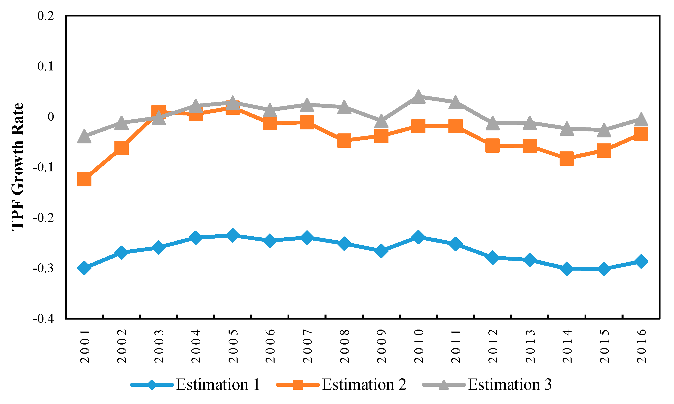
As shown in Figure 4, the rate of TFP growth in YREB under the three estimations fluctuate with tendency of up-down-up, increasing yearly before 2005, then falling to 2009, and rebounding up after 2014. In total, the changes in the rate of TFP growth in YREB under the three estimations are very small, but the four-factor estimation with carbon sequestration (0.20%) are significantly better than three-factor estimation (−3.76%) and traditional two-factor estimation (−26.55%). Compared with the estimation results of three-factor estimation and two-factor estimation, the estimation results of four-factor estimation with carbon sequestration is further improved, suggesting that carbon sequestration produce two-way synergy effect on input and output for the growth of TFP in YREB. Therefore, the CSTFP growth in YREB is obviously improved. However, due to the alternation of the two driving forces of resource-driven economic growth dominated by energy consumption and innovation-driven economic growth improved by technological progress, the rate of CSTFP growth in YREB is deadlocked in the range of 0.05%–0.3%.

5.2. Three of Four Components Drives Positively the CSTFP Growth

As shown in

Table 6. Total factor productivity growth rate and decomposition in three estimations.

	ΔTFP	ΔTP	CR	ΔTE	CR	ΔSE	CR	ΔAE	CR
Estimation 1 (two-factor)	−26.55	−25.77	−93.00	0.03	0.11	0.55	1.98	−1.36	−4.91
Estimation 2 (three-factor)	−3.76	0.90	15.25	−0.08	−1.36	0.17	2.88	−4.75	−80.51
Estimation 3 (four-factor)	0.20	1.72	18.55	2.65	28.59	0.37	3.99	−4.53	−48.87

Note: (a) CR represents contribution rate. (b) the data derives from the annual average data from 2000 to 2016.

, compared to that by two-factor estimation and three-factor estimation, the driving factors estimated by four-factor estimation reveal better results in decomposition of CSTFP growth in YREB (average annual growth of 0.2%). Among them, the rate of technological progress reaches 1.72% with a contribution rate of 18.55% to CSTFP growth, the rate of technical efficiency change reaches 2.65% with a contribution rate of 28.59%, and the rate of change in scale efficiency reaches 0.37% with a contribution rate of 3.99%. Only the rate of factor allocation efficiency change is negative (−4.53%) with contribution rate of −48.87% to CSTFP growth in YREB.

5.3. Technical Efficiency Growth Is the Primary Contributor to the CSTFP Growth

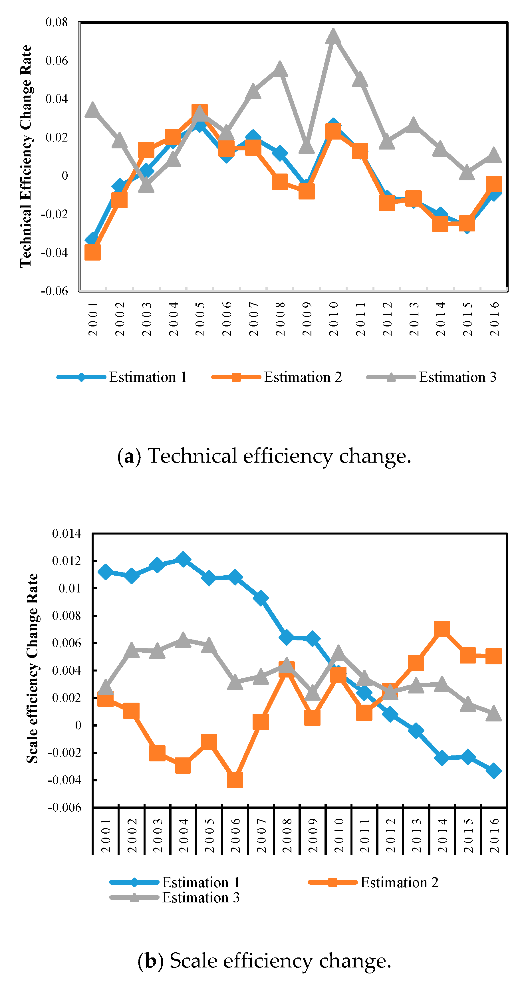
Figure 5a shows the rate of change in technical efficiency in three estimations. In comparison, the rate of technical efficiency change measured by four-factor estimation fluctuates above zero (2.65%), and it is significantly two percentage points higher than the other two estimations in each period. Technical efficiency growth is the primary contributor with the rate of 28.59% to CSTFP growth in YREB, which is supported by the four following aspects. Firstly, it is release of policy effects. The promotion of strategic measures such as “Ecological priority for green development” and “Elimination of smog for the blue sky” actively guide green development with clean production technology to increase real productivity and improve technical efficiency. Secondly, it is effective for introducing technology from the outside world (the inefficiency term OP is −0.138). By introduction, digesting and absorption of foreign technology for meeting domestic demand of development, the rate of technical efficiency change is improved. Finally, it is the result of urbanization for urban newcomers in use of technology (inefficient item UE is −0.975). The urban newcomers continue to improve their ability of employment by learning applicable technology and management experience, and this helps to accumulation of knowledge and application of technology innovation, and improvement of technological efficiency. But overall, this rate of technological efficiency change in the growth of CSTFP in YREB will be unsustainable if there is no steady increase in technological progress.

5.4. Scale Efficiency is Stabilized While Factor Allocation Efficiency is Lowered

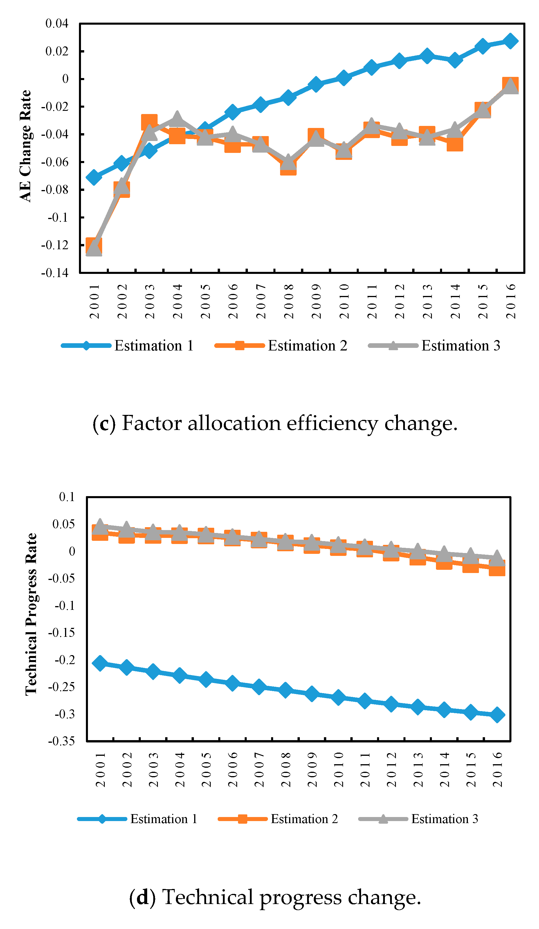
Carbon sequestration is conducive to promoting the stable growth of scale efficiency of CSTFP growth in YREB. Figure 5b shows the different trends of the scale efficiency changes in the three estimations. The rate of scale efficiency change calculated by four-factor estimation fluctuates within a narrow range of 0%–0.4%, which is relatively stable. The change rate of scale efficiency calculated by three-factor estimation has upward tendency after 2006, indicating that the change of scale efficiency brought by energy conservation, CO₂ emission reduction and low-carbon development, is significant. However, the change rate of return to scale calculated by two-factor estimation has been decreasing all the time and becomes negative after 2012, indicating that ignoring energy consumption and CO₂ emissions is not conducive to the improvement of scale efficiency. In comparison, the four-factor estimation with introducing carbon sequestration and energy consumption integrates the estimation results of the other two estimations, showing that it stabilizes the steady growth of scale efficiency of CSTFP in the YREB. However, as Figure 5c shows, among the tendency of the change rate in factor allocation efficiency in the three estimations, the results of three-factor estimation with energy consumption and CO₂ emissions (−4.75%) and four-factor estimation with carbon sequestration added (−4.53%) are significantly lower than that of traditional two-factor estimation (−1.36%), indicating that the introduction of energy consumption, CO₂ emissions, and carbon sequestration lowers the efficiency of factor allocation of CSTFP in YREB.

5.5. Distance on CSTFP Growth in Three Watershed Segments is Significant

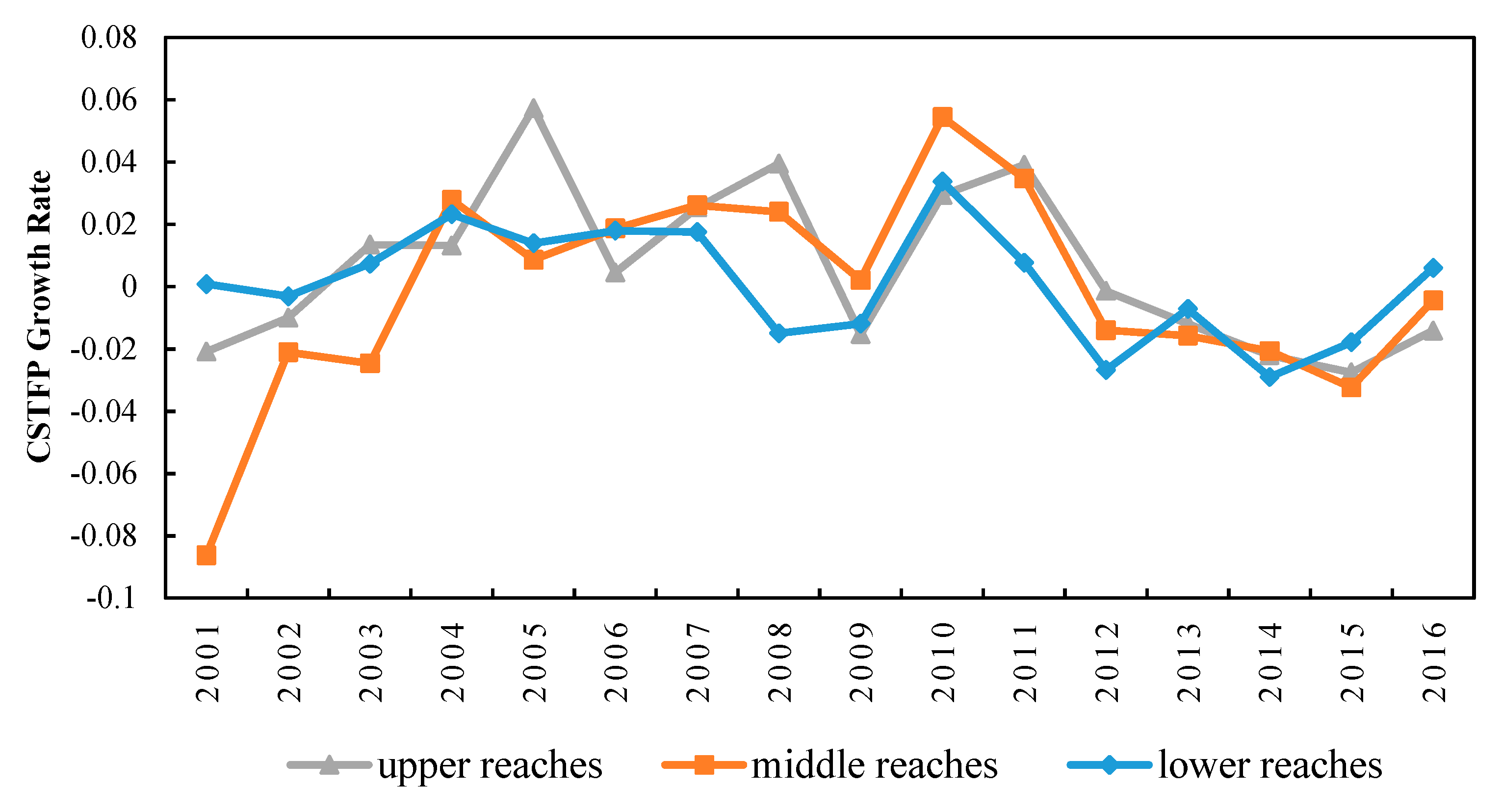
Carbon sequestration stimulate more the growth of CSTFP in the upper reaches of YREB. As Figure 6 shows, the average growth rate of CSTFP in the upper reaches of YREB is reaching 0.62%, which is the highest, three times higher than that in YREB (0.2%), while it is 0.11% in the lower reaches and -0.14% in the middle reaches. It indicates that the great capacity of carbon sequestration provided by the abundant ecological resource pool originating from the Qinghai-Tibet plateau and Yunnan-Guizhou plateau has a significant impact on the growth of CSTFP in the upper reaches of YREB, while lack of natural resource conditions in the middle reaches and the lower reaches of YREB, there is no such influence of carbon sequestration on the growth of CSTFP in those regions.

Contributors to the growth rate of CSTFP in each watershed segment of YREB are significantly different as

Table 7. Composition of CSTFP growth rate in YREB and its watershed segmental regions.

	ΔLTFP	ΔLTP	CE	ΔLTE	CE	ΔSE	CE	ΔAE	CE
Upper reaches	0.62	3.86	23.84	4.06	25.07	0.49	2.99	−7.80	−48.09
Middle reaches	−0.14	2.38	20.96	3.00	26.35	0.23	2.07	−5.75	−50.62
Lower reaches	0.11	−2.01	−48.66	0.29	7.01	0.39	9.43	1.44	34.9
the YREB	0.20	1.72	18.58	2.65	28.54	0.37	3.97	−4.53	−48.9

Note: (a) CE represents contribution rate. (b) The data is from 11 provinces and municipalities from 2000 to 2016, taking the average time of each region.

shows.

(a) In the upper reaches of YREB, the growth rate of CSTFP reaches 0.62%, three times higher than that of YREB (0.20%). The major contributors are technological progress with growth rate of 3.86% and contribution rate of 23.84%, and technical efficiency with growth rate of 4.06% and the contribution rate of 25.07%. While the weakness is factor allocation efficiency with growth rate of -7.80% and contribution rate of −48.09%.

(b) In the middle reaches of YREB, the growth rate of CSTFP is −0.14%, 2.43 times lower than that of YREB (0.20%). Its first positive contributor is technical progress with growth rate of 2.38% and contributing rate of 20.96%. Next, is technical efficiency with growth rate of 3.0% and contributing rate of 26.35%, while the foot-dragging driver is factor allocation efficiency with the growth rate of 5.75% and contribution rate of −50.62%.

(c) In the lower reaches of YREB (the Yangtze River Delta), the growth rate of CSTFP reaches 0.11%, which is 0.55 times lower than that of YREB (0.20%). The main contributor is factor allocation efficiency with growth rate of 1.44% and the contribution rate of 34.9%. While the most weakness is technological progress with growth rate of −2.01% and contribution rate of −48.66%.

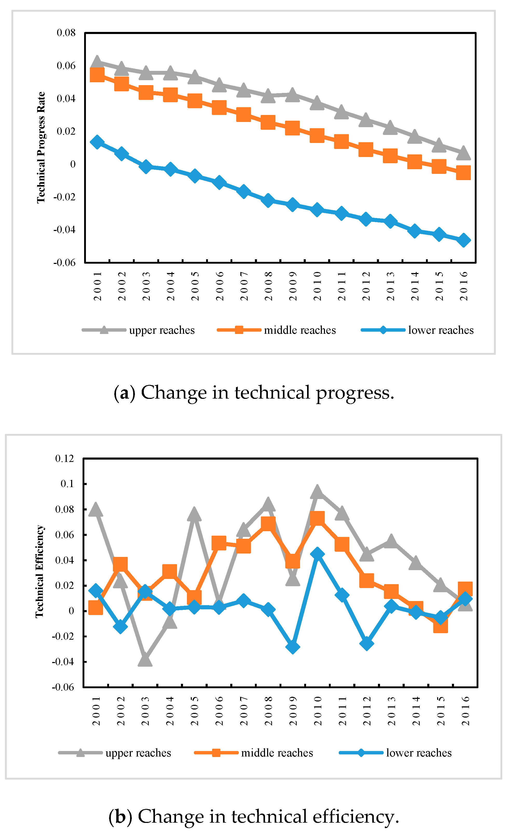
The growth rate of technological progress driver is relatively the highest in the upper reaches compared to those in the middle reaches and the lower reaches, as Figure 7a shows. It indicates that the frontier production function in the lower reaches has been moving downward on the bottom due to its slow technological progress keeping input factors and production structure unchanged since 2003, while the leading production function stays on the top and the rate of technological progress changes better in the middle reaches and the upper reaches year by year.

The growth of technical efficiency driver in the lower reaches leads the change of technical efficiency drivers in the middle reaches and the upper reaches. Figure 7b shows that the highest change rate of technical efficiency is in the lower reaches, while the lowest rate is in the upper reaches. The change rate in the middle reaches and upper reaches approaches convergent to that of the lower reaches, indicating that the growth of technical efficiency of the middle reaches and the upper reaches is led by that of the lower reaches.

Difference in the rate of scale efficiency drivers in three watersheds of YREB was reversed by year of 2009. As Figure 7c shows, the rate of change in scale efficiency in the upper and middle reaches fluctuated around zero from 2001 to 2016. Compared to that in the upper and middle reaches, the trend of change in scale efficiency in the lower reaches showed a higher tendency before 2007 but dropped down and lower than that in the middle reaches and the lower reaches after 2009, indicating that the simple expansion of scale has not promoted further economic growth for the lower reaches of YREB.

Figure 7d shows contribution of factor allocation driver to CSTFP growth in three segments of YREB. Overall, the change rate of factor allocation efficiency in each watershed segment shows a volatility. Among them, after 2003, the change rate of factor allocation efficiency in the lower reaches is above zero, indicating that the factor allocation is relatively reasonable. While the change rate of factor allocation efficiency in the middle and upper reaches is below zero all the time, reflecting that the factor allocation is not reasonable enough.

6. Discussion

6.1. Technological Progress Is Improved by Synergistic Effect of Energy Inputs and Carbon Sequestration

As Figure 5d shows, the rate of technological progress measured by three-factor estimation introducing energy consumption and four-factor estimation introducing carbon sequestration is converging and almost overlapping together in each period, and it is 25% higher than that by the results of the two-factor estimation, indicating that energy consumption has a positive correlation with carbon sequestration (co-efficient is 0.335) and this stimulates the improvement of technological progress. Because, energy consumption and industrial restructuring under the constraints of energy conservation and emission reduction (inefficiency item SI decreased from −0.923 to −1.252) stimulate related technology advance and reduce CO₂ emissions (inefficiency term CI has been reduced from 0.56 to 0.524). Meanwhile, carbon sequestration supplies clean and renewable energy to replace the fossil energy and makes energy consumption structure transited from CO₂ emissions-intensive energy to more clean and renewable energy. However, on the whole, the rate of technological progress in YREB has been declining year by year or even falling into a negative growth trend because of insufficient investment in research and development (inefficiency term R&D is stabilized from 0.109 to 0.124), and this will weaken sustainable ability of economic development in YREB.

6.2. Technical Efficiency Growth Is Benefited from Harmonious Symbiosis Influence of Carbon Sequestration

Carbon sequestration promotes harmonious symbiosis correlations with economic development and environment optimization, and this is beneficial for technical efficiency growth of CSTFP. On one end, carbon sequestration stimulates forest vegetation and ecological restoration of mountains, rivers, grasslands, wetlands, and other ecological activities, CO₂ is absorbed through photosynthesis of nature to release oxygen, and this makes ecological productivity increased and environmental improvement. On the other end, carbon sequestration creates natural resources and conditions such as carbon-rich soil, clean air, and water for agriculture, afforestation, animal husbandry, and fishery production. Under the input of labor, capital, and technology use, diversified products such as timber, food, raw materials are produced as output and create economic value for society. The function of carbon sequestration for resulting in the superposition of multitudinous input elements promotes technical efficiency and integration of natural reproduction and economic reproduction.

6.3. Inefficient Resource Allocation Is Mainly Due to Conflicts of Interest and Insufficient Coordination among Regions in YREB

In the CSTFP growth of YREB, although the concept of “ecological priority for green development” has been deeply rooted in the hearts of the people, and factor allocation efficiency has presented upward trend in total, but local governments encounter conflicts of interest in aspects of industrial development transformation, adjustment of energy structure, responsibility sharing of CO₂ emission reduction, ecological investment, and environmental governance, and each region has its own administrative boundary/territory, acts independently, lack of compromise of interests, and mutual cooperation. This results in negative growth of resource allocation efficiency (average output elasticity of capital is −1.66). Meanwhile, the unbalanced benefits being allocated between the contributors and beneficiaries of afforestation, improved forestry, or agricultural practices and ecological management (average output elasticity of CS is −1.491) deviate or restrict allocation efficiency of relevant factors improved better than before.

6.4. CSTFP Growth Is Inadequate and Uncoordinated among 11 Provinces and Municipalities of YREB

As Figure 8 shows, the upper reaches and its provinces and municipalities of Guizhou, Chongqing, and Sichuan are the leaders of the CSTFP growth of the whole basin, but inadequacies and incongruities of CSTFP growth are embodied in the middle reaches and lower reaches and relative provinces and municipalities of YREB. For example, the rate of CSTFP growth in Guizhou, Chongqing, and Sichuan reaches 3.22%, 0.87%, and 0.68%, respectively, which is higher than that in Shanghai (0.52%) and Jiangsu (0.17%). Meanwhile, the rate of CSTFP growth is negative in Yunnan (−2.3%), Hubei (−0.12%), Jiangxi (−1.09%), and Zhejiang (−0.36%), respectively. The gap of CSTFP growth rate between the highest and lowest is 5.52 percentages among different provinces and municipalities of YREB, which is driven relatively by differential growth levels of technical progress, technical efficiency, scale efficiency, and factor allocation efficiency.

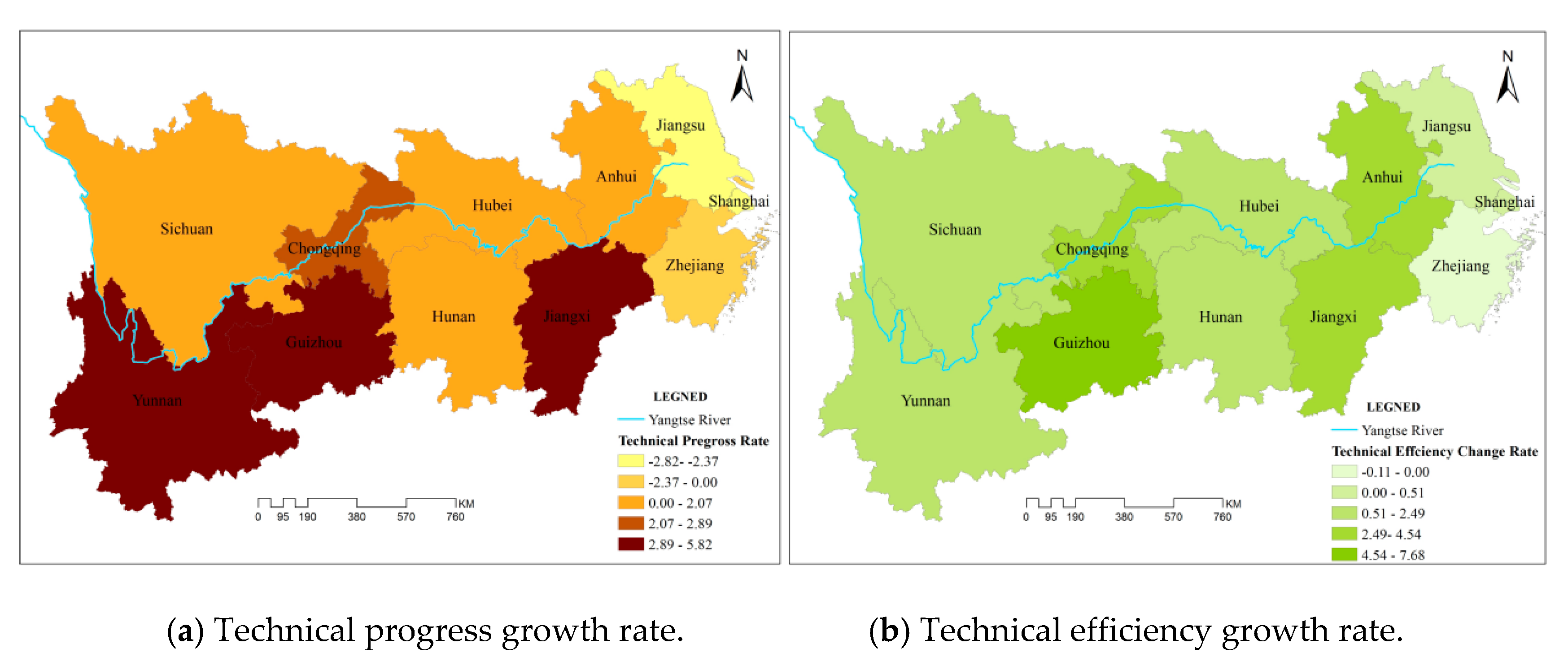
As Figure 9a shows, the higher rate of change in technical progress in the upper and middle reaches and their provinces and municipalities support the technical progress of the whole basin in YREB. Guizhou (5.85%) and Yunnan (5.17%) in the upper reaches have a higher rate of technological progress than Shanghai (−2.82%) and Jiangsu (−2.73%) in the lower reaches, where there is a gap of 8.64 percent to close because of the coefficient of intersection with time ${\beta }_{et}$ and ${\beta }_{cst}$, which is 0.0187 and 0.0269, respectively, indicating that, with increase of carbon sequestration and reduction of energy consumption, provincial level of relevant technical progress has disintegrated, multi-speed green and low-carbon technical progress growth has produced based on differential natural resources and environmental advantage in provinces and municipalities of YREB.

As shown in Figure 9b, the higher rate of change in technical efficiency in the upper and middle reaches and their provinces and municipalities leads the technical efficiency growth of the whole basin in YREB. The growth rate of technical efficiency in Shanghai (0.52%), Jiangsu (0.47%), and Zhejiang (−0.11%) in the lower reaches is significantly lower than that of the provinces and municipalities in the upper reaches and middle reaches. As Table 7 shows, based on the four-factor estimation, technical efficiency growth contributes 25.07% and 26.35%, respectively, and becomes the main source of relative CSTFP growth in the upper reaches and middle reaches of YREB, owing to the speeding up of urbanization (inefficient UE coefficient is −0.795), the second industry development (inefficient SI coefficient is −1.225), and the improvement of open outside to the world (inefficient OP coefficient is -0.138) jointly promote the technical efficiency of the upper reaches and middle reaches of YREB.

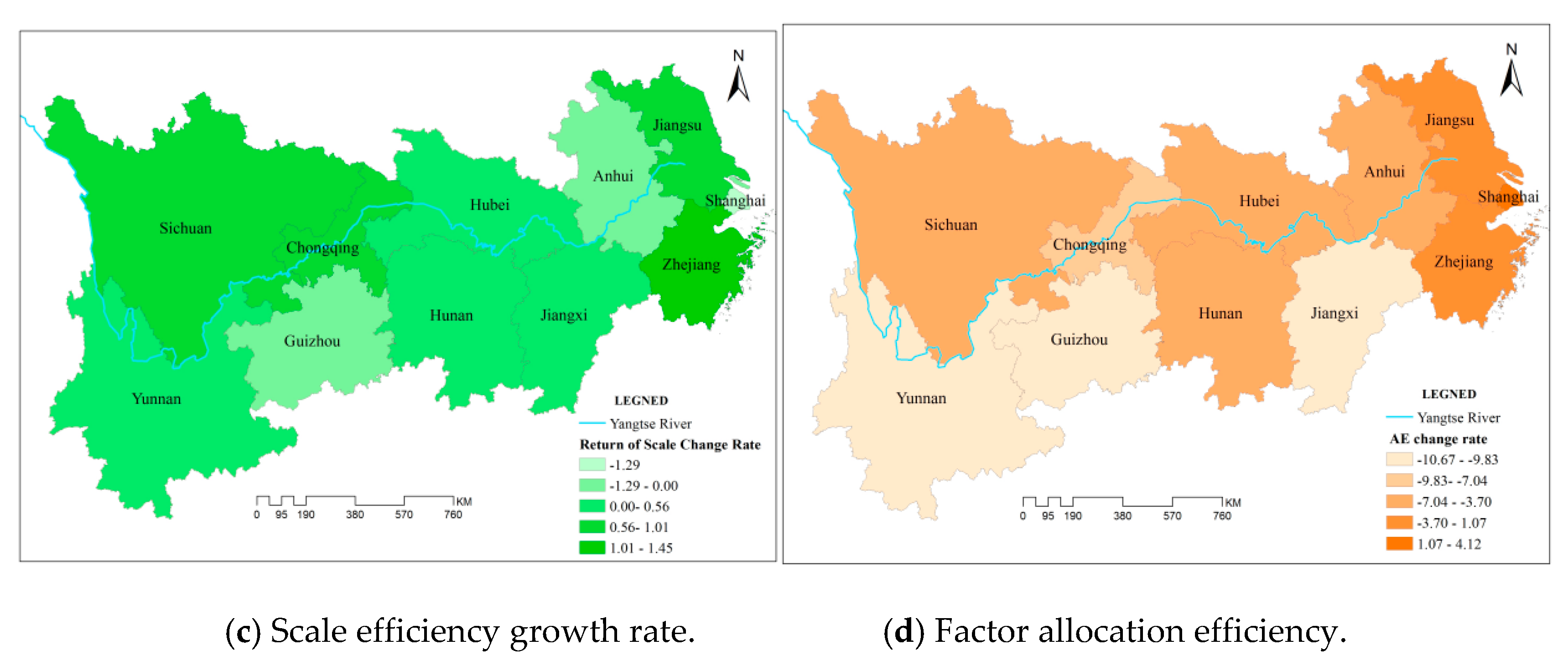
Zhejiang and Jiangsu are leaders at the growth of scale efficiency among the provinces and municipalities of YREB. As Figure 9c shows, except for Guizhou (−0.12%), Anhui (−0.47%), and Shanghai (−1.29%), the rate of change in scale efficiency in most of provinces and municipalities of YREB is positive. For example, the rate of change in scale efficiency is relatively higher in Jiangsu (1.01%) and Zhejiang (1.45%) in the lower reaches with positive contribution of 20.54% and 44.44%, respectively, to the growth rate of CSTFP, but the rate of change in scale efficiency in Shanghai is the lowest (−1.29%) with negative contribution (−14.78%) to the growth rate of CSTFP. The gap between the highest and the lowest is 2.74 percentages. Due to constraints of resources and environment, economic growth brought about by blind expansion of economic scale has been unsustainable, especially in Shanghai, Guizhou, and Anhui. Therefore, it is urgent to eliminate surplus production capacity and nurture new kinetic energy for transforming regional CSTFP growth into a high-quality mode.

Negative growth is a great challenge in the change rate of factor allocation efficiency in the provinces and municipalities of YREB. As shown in Figure 9d, only Shanghai (4.12%) and Jiangsu (1.07%) have positive change rate of factor allocation efficiency, contributing 47.15% and 21.66% to the growth rate of CSTFP, respectively. The change rate of factor allocation efficiency in other provinces and municipalities is negative, which poses a great challenge to the growth of CSTFP and high-quality development in YREB on the whole.

6.5. Total Synergies Are Not Being Unleashed Enough for Promotion of the CSTFP Growth in YREB

As Table 5 shows, labor input has a positive impact (3.278) on economic growth while capital investment has a negative impact (−0.571) in two-factor estimation with ignorance of impact of energy consumption and CO₂ emissions on TFP growth. Introducing energy consumption into endogenous variables in three-factor estimation, the impact of energy and labor on TFP growth is positive with respectively average output elasticity of 2.366 and 1.863, while that of capital on TFP growth is negative (−1.368). And further as shown in four-factor estimation with addition of carbon sequestration to endogenous variables, the average output elasticity of energy consumption (0.581) and labor (3.42) is positive, but that of carbon sequestration (−1.491) and capital(−1.66) is negative, indicating that synergies of carbon sequestration on CSTFP growth are not being unleashed enough due to the deadlock intertwined and knotted by the rival game of resources-driven economic growth dominated by fossil energy consumption and environmental-friendly economic growth driven by technological progress.

7. Conclusions and Policy Implications

7.1. Conclusions

For making it clear whether carbon sequestration is both effective at mitigating climate change and promoting economic growth, in this paper, based on carbon sequestration’s feature of harmonious symbiosis correlations between economic development and environment optimization, we firstly design an conceptual framework of CSTFP growth by taking carbon sequestration into endogenous variables from the perspective of input-–output mixes, and then set up an estimation model of CSTFP growth by adopting the stochastic frontier panel model with translog production function. Finally, we estimate and decompose CSTFP growth in YREB with 17-year data of 9 provinces and 2 municipalities under three estimations and in three watershed segments. The results show:

Compared to the result of two-factor estimation on traditional TFP growth in YREB, the CSTFP growth in YREB by four-factor estimation is obviously improved by 26.74 percentages (from −26.55% to 0.20%), which owes to carbon sequestration’s synergy effect on input and output mixes as an endogenous variable in the CSTFP growth.

Three of four components positively drive the CSTFP growth in YREB, of which technical efficiency change is the primary driver with contribution share of 28.59%, then technological progress change with contribution share of 18.55%, and scale efficiency change with contribution share of 3.99%, while factor allocation efficiency is the negative driver with reverse contribution share of −48.87% in the CSTFP growth.

The difference on the CSTFP growth in three watershed segments of YREB is significant, of which the highest is that of the upper reaches (0.62%) efficiently driven by technical efficiency change (25.07%) and technological progress change (23.84%), then that of the lower reaches (0.11%) efficiently driven by factor allocation efficiency (34.9%), and scale efficiency change (9.43%), and finally that of the middle reaches (−0.14%) efficiently driven by technical efficiency change (26.35%) and technological progress change (20.96%).

From the above analysis, technological progress is improved by synergistic effect of energy inputs and carbon sequestration, technical efficiency growth is benefited from harmonious symbiosis influence of carbon sequestration, meanwhile, inefficient resource allocation is mainly due to conflicts of interest and insufficient coordination among regions in YREB and overall synergies not being unleashed enough for driving CSTFP growth in YREB.

7.2. Policy Implications

7.2.1. Overall Synergies of Carbon Sequestration on Input–Output Mixes Should Be Given Full Play to Driving CSTFP Growth in YREB

The human activity circle is parasitic in the natural ecosystem, and both are coupled into a living community of carbon sequestration. Therefore, the following strategies should be taken to stimulate overall synergies of carbon sequestration on input-–output mixes. Firstly, afforestation is the direct strategy for the increase of carbon sequestration’s synergy effect on active use of photosynthesis of nature, including barren hills and slopes greening, forests and grasslands protection, forestry and animal husbandry production, and development of ecological agriculture and farmland protection. Secondly, river pollution control and ecological restoration is the major and urgent strategy for self-restraint of carbon sequestration’s synergy effect on water resources protection, such as pollution prevention and control and ecological restoration activities of rivers, lakes, reservoirs, wetlands, and marine protection. Thirdly, fossil fuels energy low-carbon transformation is the primary strategy for the improvement of carbon sequestration’s synergy effect on CO₂ emissions reduction and energy economic development by replacing coal power with hydro-power, wind power, and nuclear power for energy restructuring. Finally, low-carbon technologies R&D and industrialization is the fundamental strategy to improve carbon sequestration’s synergy effect on technical progress and efficiency by active promoting CCUS technology R&D and industrialization, clean production and green manufacturing, harmless disposal of garbage, resource recycling, and circular economic development.

7.2.2. Regional Close Cooperation and Harmonious Symbiosis Development Should Be Strengthened among Provinces and Municipalities of YREB

The upper reaches of YREB are rich in coal and hydro-power resources, with high forest coverage and outstanding natural carbon sink. With Chongqing and Chengdu as the strategic hubs, regional and inter-provincial cooperation should be improved for afforestation, hydro-power and wind power development, and coal cleaning. The cooperation mechanism needs to be continuously deepened jointly on development of the western region, development of the YREB, and construction of the “Belt and Road” economy and environmental conservation, for actively promoting the optimal allocation of natural ecological and economic diversified resources, and striving to improve resources allocation efficiency for CSTFP growth in YREB.

The middle reaches of YREB distribute natural rivers networks, clusters of manufacturing industry, prosperous agriculture, developed transportation, and energy industrialization. Taking the core cities of Wuhan and Nanchang as bases, focus on central rising strategy, the cross-provincial consultation, and cooperation should be improved on aspects of river pollution control and ecological restoration, fossil fuels energy transition, and low-carbon agriculture and low-carbon technologies R&D and industrialization, for continuously guiding local departments and universities, institutions, enterprises, and industry alliances actively to participate in cross-regional inter-provincial exchanges and cooperation for information sharing, joint innovation, industrial collaboration, and standard docking, and enhance resource allocation efficiency and economies of scale for CSTFP growth.

The lower reaches of YREB locate at the mouth of the sea, blessed with developed information and a strong capacity to gather resources. Setting up Shanghai as the strategic leader, the lower reaches should actively use the national strategy of the Yangtze River Delta rise to improve regional coordination and cooperation mechanism of YREB, strengthen innovation-leading, and increase local original technology while maintaining the leading edge of foreign technology absorption and digestion. R&D and industrialization should be focused on low-carbon technologies and clean energy and environmental technology for increasing the growth rate of technological progress and technological efficiency and radiating throughout the whole of YREB, and comprehensively enhancing the growth of CSTFP and modern development capacity of YREB.

References

1. Lin, B.; Ge, J. Carbon sequestration and output of China’s forestry sector: An ecological economic development perspective. Sci. Total Environ. 2019, 655, 1169–1180. [Google Scholar] [CrossRef]
2. UNFCCC. Kyoto Protocol to the United Nations Framework Convention on Climate Change. 1998. Available online: http://unfccc.int/resource/docs/convkp/kpeng.pdf (accessed on 29 November 2019).
3. Heimann, M.; Reichstein, M. Terrestrial ecosystem carbon dynamics and climate feedbacks. Nature 2008, 451, 289–292. [Google Scholar] [CrossRef]
4. Sellers, P.J.; Schimel, D.S.; Moore, B.; Liu, J.; Eldering, A. Observing carbon cycle-climate feedbacks from space. Proc. Natl. Acad. Sci. USA 2018, 115, 7860–7868. [Google Scholar] [CrossRef]
5. Seneviratne, S.I.; Donat, M.G.; Mueller, B.; Alexander, L.V. No pause in the increase of hot temperature extremes. Nat. Clim. Chang. 2014, 4, 161–163. [Google Scholar] [CrossRef]
6. Zscheischler, J.; Mahecha, M.D.; Harmeling, S.; Reichstein, M. Detection and attribution of large spatiotemporal extreme events in Earth observation data. Ecol. Inform. 2013, 15, 66–73. [Google Scholar] [CrossRef]
7. Wolf, J.; West, T.O.; Le Page, Y.; Kyle, G.P.; Zhang, X.; Collatz, G.J.; Imhoffff, M.L. Biogenic carbon flfluxes from global agricultural production and consumption. Glob. Biogeochem. Cycles 2015, 29, 1617–1639. [Google Scholar] [CrossRef]
8. Ryu, Y.; Berry, J.A.; Baldocchi, D.D. What is global photosynthesis? History, uncertainties and opportunities. Remote Sens. Environ. 2019, 223, 95–114. [Google Scholar] [CrossRef]
9. Lugoi, L.P.; Bamutaze, Y.; Martinsen, V.; Dick, B.; Almas, A.R. Ecosystem productivity response to environmental forcing, prospect for improved rain-fed cropping productivity in lake Kyoga Basin. Appl. Geogr. 2019, 102, 1–11. [Google Scholar] [CrossRef]
10. Oliver, W.K.; Atsumi, S. A carbon sequestration pathway increases carbon productivity in cyanobacteria. Metab. Eng. 2015, 29, 106–112. [Google Scholar] [CrossRef]
11. Kay, S.; Rega, C.; Moreno, G.; Herder, M.; Palma, J.H.N.; Borek, R.; Josep, C.D.; Freese, D.; Giannitsopoulos, M.; Graves, A.; et al. Agroforestry creates carbon sequestration whilst enhancing the environment in agricultural landscapes in Europe. Land Use Policy 2019, 83, 581–593. [Google Scholar] [CrossRef]
12. Wang, Q.; Su, M. The effects of urbanization and industrialization on decoupling economic growth from carbon emission—A case study of China. Sustain. Cities Soc. 2019, 51, 101758. [Google Scholar] [CrossRef]
13. Lin, B.; Xu, M. Exploring the green TFP of China’s metallurgical industry under carbon tax: A perspective on factor substitution. J. Clean. Prod. 2019, 233, 1322–1333. [Google Scholar] [CrossRef]
14. Najm, S. The green paradox and budgetary institutions. Energy Policy 2019, 133, 110846. [Google Scholar] [CrossRef]
15. Grimaud, A.; Rouge, L. Carbon sequestration, economic policies and growth. Resour. Energy Econ. 2014, 36, 307–331. [Google Scholar] [CrossRef]
16. Nishimizu, M.; Page, J.M. TFP growth, technological progress and technical efficiency change: Dimensions of productivity change in Yugoslavia, 1965–1978. Econ. J. 1982, 92, 920–936. [Google Scholar] [CrossRef]
17. Wen, G.J. TFP change in China’s farming sector: 1952–1989. Econ. Dev. Cult. Chang. 1993, 42, 1–41. [Google Scholar] [CrossRef]
18. Färe, R.; Grosskopf, S.; Norris, M.; Zhang, Z. Productivity growth, technical progress, and efficiency change in industrialized countries. Am. Econ. Rev. 1994, 84, 66–83. [Google Scholar]
19. Coelli, T.J.; Rao, D.S.P.; O’Donnell, C.J.; Battese, G.E. An Introduction to Efficiency and Productivity Analysis; Springer: New York, NY, USA, 2005. [Google Scholar]
20. Rao, G.M.; Wang, Y.; Wu, Z. Regional scientific and technological innovation mechanism of internal and external symbiosis cycle. J. Quant. Tech. Econ. 2009, 26, 87–93. (In Chinese) [Google Scholar]
21. Hailu, A.; Veeman, T.S. Non-parametric productivity analysis with undesirable outputs: An application to the Canadian pulp and paper industry. Am. J. Agric. Econ. 2001, 83, 605–616. [Google Scholar] [CrossRef]
22. Cao, J. Measuring Green Productivity Growth for China’s Manufacturing Sectors: 1991–2000. Asian Econ. J. 2007, 21, 425–451. [Google Scholar] [CrossRef]
23. Chen, S.; Golley, J. ‘Green’ productivity growth in China’s industrial economy. Energy Econ. 2014, 44, 89–98. [Google Scholar] [CrossRef]
24. Li, K.; Lin, B. Measuring green productivity growth of Chinese industrial sectors during 1998–2011. China Econ. Rev. 2015, 36, 279–295. [Google Scholar] [CrossRef]
25. Yang, W.; Shi, J.; Qiao, H.; Shao, Y.; Wang, S. Regional technical efficiency of Chinese iron and steel industry based on bootstrap network data envelopment analysis. Socio-Econ. Plan. Sci. 2017, 57, 14–24. [Google Scholar] [CrossRef]
26. Yang, Z.; Fan, M.; Shao, S.; Yang, L. Does carbon intensity constraint policy improve industrial green production performance in China? A quasi-DID analysis. Energy Econ. 2017, 68, 271–282. [Google Scholar] [CrossRef]
27. Tian, P.; Lin, B. Promoting green productivity growth for China’s industrial exports: Evidence from a hybrid input-output model. Energy Policy 2017, 111, 394–402. [Google Scholar] [CrossRef]
28. Feng, C.; Huang, J.; Wang, M. Analysis of green total-factor productivity in China’s regional metal industry: A meta-frontier approach. Resour. Policy 2018, 58, 219–229. [Google Scholar] [CrossRef]
29. Kumar, S. Environmentally sensitive productivity growth: A global analysis using Malmquist–Luenberger index. Ecol. Econ. 2006, 56, 280–293. [Google Scholar] [CrossRef]
30. Zhang, C.; Liu, H.; Bressers, H.T.A.; Buchanan, K.S. Productivity growth and environmental regulations-accounting for undesirable outputs: Analysis of China’s thirty provincial regions using the Malmquist-Luenberger index. Ecol. Econ. 2011, 70, 2369–2379. [Google Scholar] [CrossRef]
31. Wang, Z.; Feng, C. Sources of production inefficiency and productivity growth in China: A global data envelopment analysis. Energy Econ. 2015, 49, 380–389. [Google Scholar] [CrossRef]
32. Li, K.; Lin, B. Impact of energy conservation policies on the green productivity in China’s manufacturing sector: Evidence from a three-stage DEA model. Appl. Energy 2016, 168, 351–363. [Google Scholar] [CrossRef]
33. Song, M.; Peng, J.; Wang, J.; Zhao, J. Environmental efficiency and economic growth of China: A ray slack-based model analysis. Eur. J. Oper. Res. 2018, 269, 51–63. [Google Scholar] [CrossRef]
34. Mahlberg, B.; Luptacik, M.; Sahoo, B.K. Examining the drivers of total factor productivity change with an illustrative example of 14 EU countries. Ecol. Econ. 2011, 72, 60–69. [Google Scholar] [CrossRef]
35. Shen, Z.Y.; Boussemart, J.P.; Hervé, L. Aggregate green productivity growth in OECD’s countries. Int. J. Prod. Econ. 2017, 189, 30–39. [Google Scholar] [CrossRef] [Green Version]
36. Zhang, D. China’s forest expansion in the last three plus decades: Why and how? For. Policy Econ. 2019, 98, 75–81. [Google Scholar] [CrossRef]
37. Aigner, D.J.; Lovell, C.A.K.; Schmidt, P. Formulation and estimation of stochastic frontier production function models. J. Econom. 1977, 6, 21–37. [Google Scholar] [CrossRef]
38. Meeusen, W.; van den Broeck, J. Efficiency estimation from Cobb-Douglas production functions with composed error. Int. Econom. Rev. 1977, 18, 435–444. [Google Scholar] [CrossRef]
39. Forsund, F.R.; Lovell, C.A.K.; Schmidt, P. A survey of frontier production functions and of their relationship to efficiency measurement. J. Econom. 1980, 13, 5–25. [Google Scholar] [CrossRef]
40. Schmidt, P. Frontier production functions. Econ. Rev. 1986, 4, 289–328. [Google Scholar] [CrossRef]
41. Bauer, P.W. Recent developments in the econometric estimation of frontiers. J. Econom. 1990, 46, 39–56. [Google Scholar] [CrossRef]
42. Battese, G.E. Frontier production functions and technical efficiency: A survey of empirical applications in agricultural economics. Agric. Econom. 1992, 7, 185–208. [Google Scholar] [CrossRef] [Green Version]
43. Battese, G.E.; Coelli, T.J. A model for technical inefficiency effects in a stochastic frontier production function for panel data. Empir. Econ. 1995, 20, 325–332. [Google Scholar] [CrossRef] [Green Version]
44. Coelli, T.J. A computer program for frontier production function estimation: FRONTIER Version 2.0. Econ. Lett. 1992, 39, 29–32, (In North-Holland). [Google Scholar] [CrossRef]
45. Arazmuradov, A.; Martini, G.; Scotti, D. Determinants of TFP in former Soviet Union economies: A stochastic frontier approach. Econ. Syst. 2014, 38, 115–135. [Google Scholar] [CrossRef] [Green Version]
46. Zhang, Q.; Xu, Z.; Feng, T.; Jiao, J. A dynamic stochastic frontier model to evaluate regional financial efficiency: Evidence from Chinese county-level panel data. Eur. J. Oper. Res. 2015, 241, 907–916. [Google Scholar] [CrossRef]
47. Chen, Z.; Barros, C.P.; Borges, M.R. A Bayesian stochastic frontier analysis of Chinese fossil-fuel electricity generation companies. Energy Econ. 2015, 48, 136–144. [Google Scholar] [CrossRef]
48. Lin, B.; Long, H. A stochastic frontier analysis of energy efficiency of China’s chemical industry. J. Clean. Prod. 2015, 87, 235–244. [Google Scholar] [CrossRef]
49. Li, H.Z.; Tian, X.L.; Zou, T. Impact analysis of coal-electricity pricing linkage scheme in China based on stochastic frontier cost function. Appl. Energy 2015, 151, 296–305. [Google Scholar] [CrossRef]
50. Glass, A.J.; Kenjegalieva, K.; Sickles, R.C. A spatial autoregressive stochastic frontier model for panel data with asymmetric efficiency spillovers. J. Econom. 2016, 190, 289–300. [Google Scholar] [CrossRef] [Green Version]
51. Pieri, F.; Vecchi, M.; Venturini, F. Modelling the joint impact of R&D and ICT on productivity: A frontier analysis approach. Res. Policy 2018, 47, 1842–1852. [Google Scholar]
52. Balliauw, M.; Meersman, H.; Onghena, E.; Voorde, E.V. US all-cargo carriers’ cost structure and efficiency: A stochastic frontier analysis. Transp. Res. Part A 2018, 112, 29–45. [Google Scholar] [CrossRef]
53. Tsionas, M.G.; Mallick, S.K. A Bayesian semiparametric approach to stochastic frontiers and productivity. Eur. J. Oper. Res. 2019, 274, 391–402. [Google Scholar] [CrossRef]
54. Boyd, G.A.; Lee, J.M. Measuring plant level energy efficiency and technical change in the U.S. metal-based durable manufacturing sector using stochastic frontier analysis. Energy Econ. 2019, 81, 159–174. [Google Scholar] [CrossRef] [Green Version]
55. Ondrich, J.; Ruggiero, J. Efficiency measurement in the stochastic frontier model. Eur. J. Oper. Res. 2001, 129, 434–442. [Google Scholar] [CrossRef]
56. Kumbhakar, S.C. The specification of technical and allocative inefficiency in stochastic production and profifit frontiers. J. Econom. 1987, 34, 335–348. [Google Scholar] [CrossRef]
57. Kumbhakar, S.C. Production frontiers, panel data, and time-varying technical inefficiency. J. Econom. 1990, 46, 201–211. [Google Scholar] [CrossRef]
58. Bai, C.; Du, K.; Yu, Y.; Feng, C. Understanding the trend of total factor carbon productivity in the world: Insights from convergence analysis. Energy Econ. 2019, 81, 698–708. [Google Scholar] [CrossRef]
59. Miao, Z.; Chen, X.; Baležentis, T.; Sun, C. Atmospheric environmental productivity across the provinces of China: Joint decomposition of range adjusted measure and Luenberger productivity indicator. Energy Policy 2019, 132, 665–677. [Google Scholar] [CrossRef]
60. Shi, X.; Li, L. Green TFP and its decomposition of Chinese manufacturing based on the MML index: 2003–2015. J. Clean. Prod. 2019, 222, 998–1008. [Google Scholar] [CrossRef]
61. Li, W.; Wang, W.; Wang, Y.; Mustafa Ali, M. Historical growth in total factor carbon productivity of the Chinese industry: A comprehensive analysis. J. Clean. Prod. 2018, 170, 471–485. [Google Scholar] [CrossRef]
62. Wang, Q.; Zhang, C.; Cai, W. Factor substitution and energy productivity fluctuation in China: A parametric decomposition analysis. Energy Policy 2017, 109, 181–190. [Google Scholar] [CrossRef]
63. Su, B.; Ang, B.W. Multiplicative decomposition of aggregate carbon intensity change using input-output analysis. Appl. Energy 2015, 154, 13–20. [Google Scholar] [CrossRef]
64. Su, B.; Ang, B.W. Multi-region comparisons of emission performance: The structural decomposition analysis approach. Ecol. Indic. 2016, 67, 78–87. [Google Scholar] [CrossRef]
65. Su, B.; Ang, B.W. Multiplicative structural decomposition analysis of aggregate embodied energy and emission intensities. Energy Econ. 2017, 65, 137–147. [Google Scholar] [CrossRef]
66. Zhang, Z.; Ye, J.L. Decomposition of environmental TFP growth using hyperbolic distance functions: A panel data analysis for China. Energy Econ. 2015, 47, 87–97. [Google Scholar] [CrossRef]
67. Debreu, G. The coefficient of resource utilization. Econometrica 1951, 19, 273–292. [Google Scholar] [CrossRef]
68. Anga, F.; Kerstens, P.J. Decomposing the Luenberger-Hicks-Moorsteen TFP indicator: An application to U.S. agriculture. Eur. J. Oper. Res. 2017, 260, 359–375. [Google Scholar] [CrossRef]
69. Diewert, W.E.; Fox, K.J. Decomposing productivity indexes into explanatory factors. Eur. J. Oper. Res. 2017, 256, 275–291. [Google Scholar] [CrossRef]
70. Boussemart, J.-P.; Leleu, H.; Shen, Z. Environmental growth convergence among Chinese regions. China Econ. Rev. 2015, 34, 1–18. [Google Scholar] [CrossRef]
71. Cheng, Z.H.; Li, L.; Liu, J.; Zhang, H. Research on energy directed technical change in China’s industry and its optimization of energy consumption pattern. J. Environ. Manag. 2019. [Google Scholar] [CrossRef]
72. NBS. China Statistical Yearbook 2000–2016; Chongqing Statistical Yearbook 2000–2016; Sichuan Statistical Yearbook 2000–2016; Guizhou Statistical Yearbook 2000–2016; Yunan Statistical Yearbook 2000–2016; Hubei Statistical Yearbook 2000–2016; Hunan Statistical Yearbook 2000–2016; Jiangxi Statistical Yearbook 2000–2016; Anhui Statistical Yearbook 2000–2016; Shanghai Statistical Yearbook 2000–2016; Jiangsu Statistical Yearbook 2000–2016; Zhejiang Statistical Yearbook 2000–2016; China Statistics Press: Beijing, China, 2000–2016.
73. NDRC. Price Yearbook of China 2000–2016; Editorial Department of Price Yearbook of China Press; Chinese Price Society: Beijing, China, 2000–2016.
74. Shan, H. Re-estimation of China’s capital stock k: 1952–2006. J. Quant. Tech. Econ. 2008, 25, 17–31. (In Chinese) [Google Scholar]
75. Development and Reform Office of China. Guidelines for the Preparation of Provincial Greenhouse Gas Inventories; No. 1041; Development and Reform Office Climate: Beijing, China, 2011.
76. Xie, H.Y.; Chen, X.S.; Lin, K.R.; Hu, Y.Y. Ecological footprint of fossil energy and electric power based on carbon cycle. Acta Ecol. Sin. 2008, 1729–1735, (In Chinese with English Abstract). [Google Scholar] [CrossRef]
77. He, H.; Pan, Y.; Zhu, W.; Liu, X.; Zhang, Q.; Zhu, X. Measurement of terrestrial ecosystem service value in China. Acta Ecol. Appl. Sin. 2005. [Google Scholar] [CrossRef]
78. Mei, X.Y.; Zhang, X.F. Carbon storage and carbon sequestration of typical wetland vegetation in the Yangtze estuary—A case study of the reed belt in dongtan, chongming. Chin. J. Ecol. Agric. 2008, 16, 269–272, (In Chinese with English Abstract). [Google Scholar] [CrossRef]
79. Tian, Y.Y.; Zhang, J.Q. Differentiation of net carbon effect in agricultural production in China. Chin. J. Nat. Resour. 2013, 28, 1298–1309, (In Chinese with English Abstract). [Google Scholar]
80. 80. Mohan Dey, M.; Javien Paraguas, F.; Srichantuk, N.; Xinhua, Y.; Bhatta, R.; Thi Chau Dung, L. Technical efficiency of freshwater pond polyculture production in selected Asian countries: Estimation and implication. Aquac. Econ. Manag. 2005, 9, 39–63. [Google Scholar] [CrossRef]
Figure 1. The conceptual framework of carbon sequestration total factor productivity (CSTFP) growth estimation.
Sustainability 11 06809 g001
Figure 2. Map of the Yangtze River Economic Belt and its three watershed segments.
Sustainability 11 06809 g002
Figure 3. Historical trend of selected indicators in YREB, 2000–2016.
Sustainability 11 06809 g003
Figure 4. The growth rate of CSTFP in YREB under three estimations.
Sustainability 11 06809 g004
Figure 5. Comparison of different drivers under three estimations in YREB.
Sustainability 11 06809 g005aSustainability 11 06809 g005b
Figure 6. The rate of CSTFP growth in three watershed segments of YREB.
Sustainability 11 06809 g006
Figure 7. Drivers decomposition of CSTFP in YREB.
Sustainability 11 06809 g007aSustainability 11 06809 g007b
Figure 8. CSTFP growth rate among 11 provinces in YREB.
Sustainability 11 06809 g008
Figure 9. CSTFP growth drivers among 11 provinces in YREB (label is the same as Figure 8).
Sustainability 11 06809 g009aSustainability 11 06809 g009b