1. Introduction
The concept of a low carbon economy has come into existence to cope with numerous environmental challenges. Due to government regulations and public awareness, enterprises have realized the importance of introducing low-carbon operations and sustainability into their management objectives. Agi et al. [
1] conducted a study on Australian firms and found two main motives that caused enterprises to shift towards green development. The first motive is to comply with environmental regulations, and the second motive is to achieve a competitive edge. Diabat et al. [
2] indicated that the sustainable supply chain management (SSCM) system could ensure environmentally friendly practices in traditional supply chains with essential enablers. On the one hand, government policies and regulations, such as carbon caps, are putting pressure on enterprises to incorporate environmental factors into their business models. On the other hand, a number of enterprises have made sustainable green operations as their competitive advancement. In supply chains, several activities produce carbon emissions, for example, transportation and warehousing. Hence, it is critical to manage and control carbon emissions in supply chain operations.
Global trade boosts have shifted the short-distance supply chain within a country to long distance supply chain between countries [
3]. This change has resulted in an increase in the lead time and has accelerated the fluctuation. The lead time is also called replenishment delay, which is the time gap between sending an order and receiving it. Existing studies demonstrate that lead time is a key factor that affects supply chain performance [
4]. If the lead time is uncertain, the situation is complex from both the cost and service perspectives. Our research is motivated by the growing concern of business, which is forcing business enterprises to reduce carbon emission cost in their supply chain network. Therefore, this paper includes carbon emission costs as one of the supply chain performance indicators. Some studies [
5,
6] have demonstrated that the uncertain lead time is directly related to supply chain performance. Therefore, this paper examines the effect of uncertain lead time on carbon emission costs. Further, the paper investigates whether the effect of lead time increase on the behavior of carbon cost emissions is the same as the behavior of inventory costs and service levels or not.
When both market demand and lead time are uncertain, the supply chain system becomes more complicated and dynamic with time [
7]. The traditional operational method makes it difficult to explore the complicated supply chain system. System dynamics provides a new way to study complex systems. The discipline of system dynamics was founded in 1956 by Professor Forrester of the Massachusetts Institute of Technology. The system dynamics discipline integrates systems theory, cybernetics, information theory, and organization theory with the help of computer technology. The system dynamics model can also show the dynamic behavior of the object system. The system dynamics can be used to better analyze non-linear systems which are caused by many real situations in the supply chain system, such as stochastic lead time, uncertain demand, non-negative order, etc. In this study, we applied a system dynamics method to build a supply chain model and explore the dynamic change trend of supply chain performance indicators, including inventory cost, service level, and carbon cost, under uncertain lead times.
The reminder of this paper is organized as follows:
Section 2 presents an overview of the relevant literature.
Section 3 presents the assumptions and models and introduces the performance indicators;
Section 4 conducts model analysis and numerical simulations.
Section 5 focuses on the analysis of experimental results. Finally,
Section 6 summarizes the main research conclusions and proposes several future research directions.
2. Literature Review
Research was conducted on how to reduce the negative impact on the environment during supply chain operations [
8,
9]. Quite a number of studies focus on transportation studies [
10,
11,
12]. This paper mainly discusses the dynamic change of carbon emission cost in an uncertain supply chain environment with stochastic lead time, and explores the inventory management approach to buffer the fluctuation.
In the research on carbon inventory management, the focus has been on newsvendor models and EOQ (economic order quantity) models [
13,
14,
15]. Song et al. [
16] analyzed a newsvendor model and demonstrated that it is possible to achieve multiple targets, including carbon emission reduction, cost saving, and profit improvement at the same time by applying a suitable order policy. Chen et al. [
17] also found that there are some conditions under which the reduction in carbon emissions is greater than the increase in cost. Hovelaque et al. [
18] presented a novel model which considered the relationship among inventory policy, carbon emissions, and price account. They found that certain environmental policies can significantly decrease total carbon emissions.
Most recent research focuses on different operational factors in the supply chain while simultaneously considering carbon emissions. Benjaafar et al. [
19] integrated carbon emissions into supply chain operational process with inventory management, production, and procurement. They also modified traditional models to account for both general cost and carbon emissions. Diabat et al. [
20] proposed a genetic algorithm approach for supply chain integration while considering carbon emissions. They considered multiple scenarios such as different demand models and multiple distribution centers. Park et al. [
21] investigated punishment mechanism in supply chain structure and found that supply chain members are affected differently by carbon emission reduction. Konur et al. [
22] incorporated environmental factors into a supply chain control model with uncertain demand to study the effect of logistics policies and supplier selection on environmental performance. Xu et al. [
23] considered demand preferences in low carbon supply chain management to analyze the effect of consumer preference on inventory cost. Hoen et al. [
24] studied the effects of transportation facilities on carbon emissions under uncertain demand conditions. They showed that the lead time directly affects carbon emissions on a transport facility. Sarkar et al. [
25] reached a similar conclusion. Finally, Arikan et al. [
26] studied environmental effects related to lead time uncertainty for transportation facilities.
Recent studies on low carbon inventory management have begun to account for an uncertain lead time effect, but the research in this field is not sufficient. Many existing studies were based on order-up-to-level inventory models. For example, Chatfield et al. [
27] studied stochastic lead time and established order-up-to-level inventory models of periodic replenishment. They conducted computer experiments to explore the impact of stochastic lead time on the inventory system. The results showed that the uncertainty of lead time aggravates the fluctuation of ordering quantity. Yet, efficient sharing of quality information is beneficial to reduce the fluctuation. Du et al. [
28] extended the demand model to an autoregressive moving average model (ARMA) with independent and identically distributed lead times. However, these two studies both used the order fluctuation as the only evaluation indicator to study the uncertain lead time effect. Many studies added the bullwhip effect as the evaluation index. The bullwhip effect is the magnified effect of the demand information distortion while moving from downstream to upstream in the supply chain. The bullwhip effect states that a small fluctuation in demand at the downstream level (i.e., at a retailer level) creates larger fluctuations in demand at the upstream level (i.e., wholesale, distributor, manufacturer, and raw material supplier levels). In supply chain management, each player has limited information over demand and, thus, the fluctuating demand pattern at any supply chain link influences the entire supply chain with its forecasting inaccuracy (i.e., ordering too much or ordering too less). It is considered to be one of the main factors that weakens supply chain performance, because it creates either excess inventory or shortages in the whole supply chain network. A detailed explanation about the bullwhip effect can be found in the literature [
27]. Boute et al. [
29] considered both order fluctuation and inventory fluctuation. By conducting numerical simulation experiments, they found that the bullwhip effect and inventory costs can be reduced at the same time. However, this study assumed that the supply chain is linear and that there are no order crossovers. In fact, an in-depth study by Saldanha et al. [
30] affirmed that the order crossover is a common phenomenon. Chaharsooghi et al. [
31] investigated the bullwhip effect in multi-echelon supply chain models and concluded that random lead time has a greater impact on bullwhip effect over fixed lead time.
Jian et al. [
32] considered the influence of the randomness of lead time on the inventory model for perishable drugs. Through empirical and sensitivity analysis, they determined that the weight-distribution values of the shelf life of perishable drugs and the service level are reasonable. Spiegler et al. [
33] discussed the influence of lead time uncertainty on order quantity, inventory level, and work-in-process quantity. Assuming demand is stable, they followed the small disturbance principle to probe lead time disturbance related to system output, and they found that the order quantity, inventory level, and work-in-process quantity increase with the lead time. Moreover, the reduction in lead time can result in a dynamic change of damping. This result implies that, although reducing the lead time can improve system performance, a flexible management plan is required to avoid unnecessary system turbulence. The above study provides a theoretical basis for setting up the parameter in this paper. Dejonckheere et al. [
34] proved that an order-up-to-level order policy creates a bullwhip effect. However, if two feedback loops are introduced to the order policy, the bullwhip effect can be weakened and, sometimes, even eliminated. This order policy is called APVIOBPCS (automatic pipeline, variable inventory, and order based on production control system). The APVIOBPCS model has two feedback loops to control the order quantity by discrepancies in inventory and work-in-process. In addition, by changing the adjustment parameters, APVIOBPCS policy clusters are generated as various ordering policies. When the adjustment parameters of inventory and work-in-process inventory are both 1, it becomes an order-up-to-level policy. The APVIOBPCS model has been applied in practice and in real time [
35,
36,
37].
This paper differs from the existing studies in the following aspects. First, the model in this paper considers both uncertain demand and uncertain lead time, which is near reality situation. Correspondingly, there is an order crossover phenomenon in the supply chain model which only emerges when lead time is stochastic. These conditions make the model more complex and nonlinear. Second, this paper introduces carbon cost into the supply chain model as a new systematic performance indicator. It compares average cost and average service level change to carbon cost change under varying supply chain environments. This paper also adopts the system dynamics method to discuss the impact of stochastic lead time on supply chain inventory system, and also find more suitable order policies than the traditional order method, which can dampen the negative effect of uncertain lead time.
3. Inventory Control System Model Considering Stochastic Lead Times
3.1. Assumptions
In order to explore the impact of stochastic lead times on supply chain inventory systems, this paper constructed a three-stage supply chain with a distributor as the focal point in a periodic continuous review system based on the APVIOBPCS model. The proposed model makes the following assumptions:
Assumption 1. At the beginning of a single period, the distributor receives the products from the manufacturer, and the distributor’s ordering plan is submitted to the manufacturer at the end of the period; at the same time, the system state is updated.
Assumption 2. The upstream manufacturer has abundant production capacity and can fully meet the orders from the distributor without shortages.
Assumption 3. The downstream retailer demand follows normal distribution , and the demand of each period may not be fully met due to variable market demand.
Assumption 4. The demand forecasting for the next period is based on the exponential smoothing method, with the smoothing factor.
Assumption 5. The distributor supplies products to the retailer with the SFS model (supply from stock). That is, the minimum of demand and current inventory is supplied. The shortage will not be replenished in the current period, and it needs to be submitted by downstream retailer in the next period in the form of new demand orders. Hence, inventory is allowed to take negative value. It is noted that this is consistent with business practice.
Assumption 6. The distributor’s orders are subject to non-negative constraints. In business reality, it can be interpreted as not allowing returns.
3.2. Stochastic lead times
This paper investigates the influence of stochastic lead times on the performance of supply chain inventory level. While introducing stochastic lead times into the model, it is essential to consider the allowance of order crossover. In order crossover, the sequence of order arrival can be different from the sequence of order placement. Order crossover is due to stochastic lead time. Due to randomness, multiple order batches from several previous periods could arrive in one period at the same time, or the distributor could receive those orders in advance, which are placed in a later period. According to a global logistics survey [
38], crossover orders accounted for more than 40% of total orders. Thus, this paper facilitates the order crossover in the supply chain system.
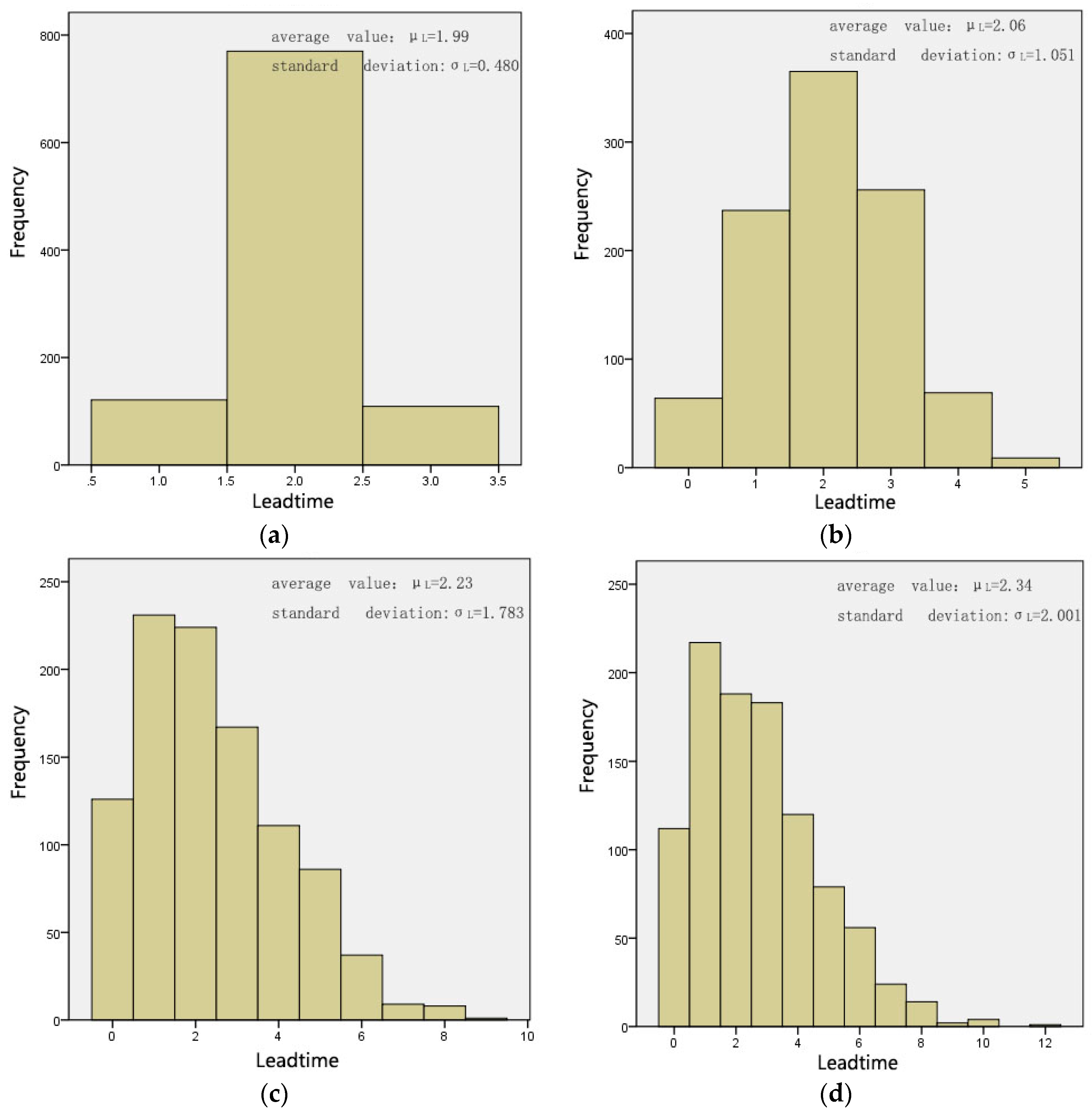
The logistics data survey in study [
38] shows that the lead time distribution is random. Some of the lead time distributions are normal, and some of them are close to normal with long tail. This paper simulates stochastic lead time distributions based on the observations found in the study [
38]. We chose several values for standard deviation (
) to simulate different levels of lead time uncertainty with the same average lead time value (
).
Figure 1 shows the four distributions with different standard deviations in our experiments. The symbol
represents the corresponding lead time in period
, with the minimum denoted by 0 and the maximum denoted by
. According to the supply chain event process of this model, a single period in the system starts with the distributor receiving the products from the manufacturer and ends at the distributor issuing the current order plan to the supplier. Submission of the order plan is the last step of each period. Thus, there is a natural delay in the periodic cycle when the distributor receives the homologous products of his order plan. Therefore, the earliest and the latest arrival times of the products in the order plan submitted in period
are recorded as
and
, respectively.
In simulation experiments, the lead time uncertainty can be simulated by the following steps:
Step 1: The distribution of random lead time is assumed in the model. MATLAB is used to generate n random numbers representing the lead time in the period; these are stored in an array . There are five presumed types of lead time distributions corresponding to five experiments.
Step 2: Next, the array is introduced into the basic inventory simulation model, and the delay, corresponding to the order quantity and determined at the end of the simulation period t, is denoted as .
Step 3: Since each is generated in step 1, the arrival time of can be calculated at the beginning of each period and recorded in the arrival time array as: .
Step 4: In each period, the array from period to period is checked to determine whether equals . If so, the corresponding arrival quantity can be included in the current inventory. Otherwise, it is counted as the work-in-process inventory.
3.3. Models
The basic inventory model of this paper is based on the APVIOBPCS (Automatic Pipeline Inventory and Order based Production Control System) model family. The APVIOBPCS model is a collection of inventory policies, which can express different inventory policies with different parameter settings. The common order-up-to-level inventory order policy, which has been used in practice, is also a form of APVIOBPCS.
The core enterprise of the supply chain model in this paper is the distributor. The upstream of the distributor is the manufacturer and downstream is the retailer. According to the principle of the APVIOBPCS production control, the model is assumed to be a periodic review system. The state of each system variable would be updated as the following process.
At the beginning of the period
, the distributor receives the previously placed orders. Due to the order crossover as mentioned above, in period
, products purchased in multiple historical periods might arrive at the same time, or the distributor may receive the recently ordered products in advance. Accordingly, the arrival quantity
is equal to the sum of orders the manufacturer is delivering
before several periods based on the
, as shown in Equation (1). Then, the distributor can count the inventory
at the beginning of period
using Equation (2), which is the sum of the inventory at the end of the last period and the current arrivals.
The distributor delivers the products to the retailer from stock to meet market demand
, and delivery volume
is the minimum of
and the initial inventory
at period
, as expressed in Equation (3). If the value of
is less than
, stock out
occurs, which can be calculated using Equation (4). In addition, according to the assumptions in
Section 3.3, the shortage
in the current period would not be fulfilled by the distributor in the next period. When there is a shortage
in the current period, products are replenished in the form of new demand orders submitted by downstream retailers in the next periods. This policy is consistent with the practice used in many manufacturing industries. Therefore, the shortage
is not in Equation (3).
Equation (5) denotes the ending inventory
of the period
t. The ending inventory
is the minimum of 0 and the difference between the
and the
. The work-in-process inventory
represents the products that have been dispatched by the manufacturer but have not yet reached the distributor.
can be obtained by subtracting the current arrivals
from the sum of the previous work-in-process inventory
and the order quantity
using Equation (6). After sending out the demand quantity of the market and ensuring
and
, the next market demand
is forecasted. The exponential smoothing method is used to forecast demand with the smoothing factor
, as in Equation (7).
Equation (8) reveals the mathematical model of the order policy, which is the key point of the APVIOBPCS model. In order to reduce errors caused by the forecast, two feedback loops were introduced into the model: Adjustment for stock and adjustment for work-in-process. The adjustments for stock and work-in-process inventory discrepancies are represented into the order equation
with the parameters
and
, respectively. Hence,
and
are the parameters of the adjustment for
and
, respectively.
The target inventory in the model is denoted by
, where
is the average demand and the parameter
is the correlation factor between the target inventory and demand
. When
, the target inventory is 0, and the system achieves the ideal state of “zero inventory”. When the lead time is uncertain, the work-in-process inventory cannot be overlooked. It would put an important impact on the overall inventory level and performance of the supply chain. The forecasting demand of the products
and the average lead time
were set as the objective work-in-process inventory to reduce the uncertainty of order decision caused by lead time fluctuation. The parameter combination
corresponds to different ordering policies. Earlier research results [
39] proved that these parameters and their correlation can impact or determine the stability and performance of a supply chain. Furthermore, when
, the policy is called a POUT policy, which is used in this paper.
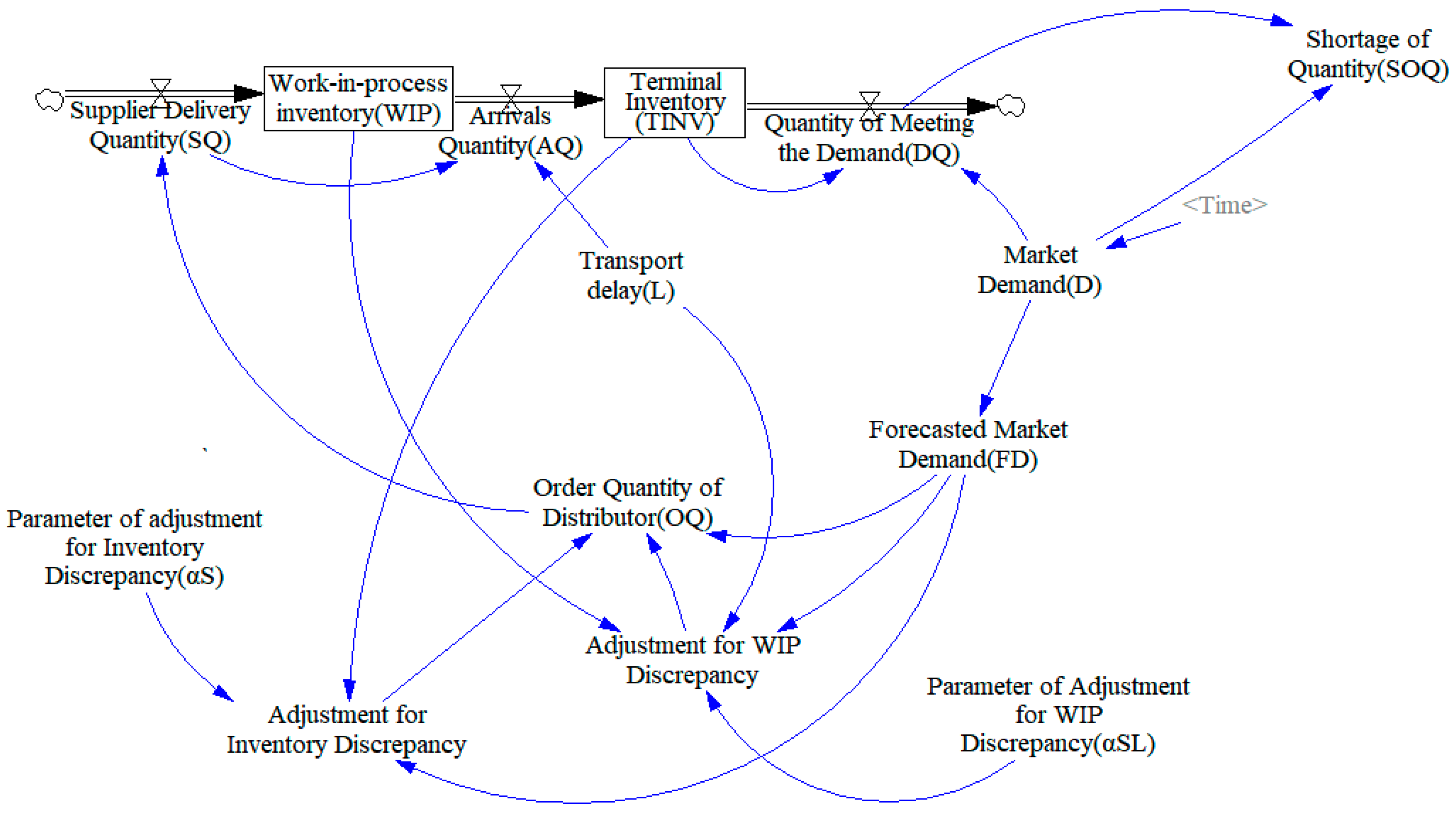
The main variables and parameters of the model are listed in
Table 1. The correlation among the variables is shown in an inventory system dynamics model diagram as in
Figure 2.
3.4. System Performance Indicators
3.4.1. The Carbon Cost
In this paper, the carbon cost
is introduced as one of the performance indicators for the system, and the system’s carbon cost in the model consists of two components. The first component is the transportation carbon cost, and the other is the inventory carbon cost. The transportation carbon cost
mainly comes from the transportation carbon emissions
generated by vehicle fuel consumption. Bao et al. [
40] proved that the fuel consumption is affected by vehicle load. Equation (9) specifies the mathematical relationship between the fuel consumption per unit distance
and the load
of a truck under the condition of a non-full load. The fuel consumption in a non-full load and a full-load are denoted as
and
, respectively. Meanwhile,
is a constant, emblematizing the maximum load weight of trucks. In the experiment, the total number of trucks
could be calculated from the number of products transported and the weight. According to the Law of Conservation of Elements in chemistry, in a chemical reaction, the kinds and qualities of the elements participating in the reaction remain unchanged. By tracing the carbon atoms in the chemical reaction equation, the carbon emission
per unit of fuel consumption can be converted. After determining the transportation mileage from the manufacturer to the distributor, the total transport carbon emission
can be obtained using Equation (10). Furthermore, according to the carbon emission policies of a few countries and regions, the carbon tax
is multiplied with
to get the transportation carbon cost
using Equation (11).
The inventory carbon cost
is the other component of
. In inventory management, carbon is released by the electrical energy consumption of relevant facilities and equipment, such as refrigeration cabinet, room temperature cabinet, automatic stacker, etc. According to the literature [
41], the carbon emission per inventory product can be calculated from the conversion relationship between electricity consumption and carbon emissions. In addition, the sensitivity analysis shows that the carbon emissions per product only affect the total cost of inventory carbon emissions, and would not change its fluctuation trend, which is the focus of this paper. In this paper,
is defined as the inventory carbon cost per product. The inventory carbon cost
of the period
can be obtained using Equation (12). Equation (13) represents the total inventory carbon cost
, while Equation (14) aggregates the total carbon cost
.
3.4.2. Average Inventory Cost
Most scholars define the system inventory cost as the combination of inventory holding cost per unit
and shortage cost per unit
. This paper adopts the same method for the calculation of inventory cost, as defined in Equation (15).
3.4.3. Average Service Level
Macchion et al. [
42] assumed the service level
of each period to be 0 or 1. In the case of shortages, the service level is considered 0. Otherwise, it is considered 1. In this paper, shortage is introduced to further quantify the service level. As shown in Equation (16), the ratio of shortage
and demand
of period
is considered when calculating the service level
. Furthermore, the average service level
ASL is calculated using Equation (17):
5. Analysis of Experimental Results
5.1. Effect of Stochastic Lead Times on System Performance
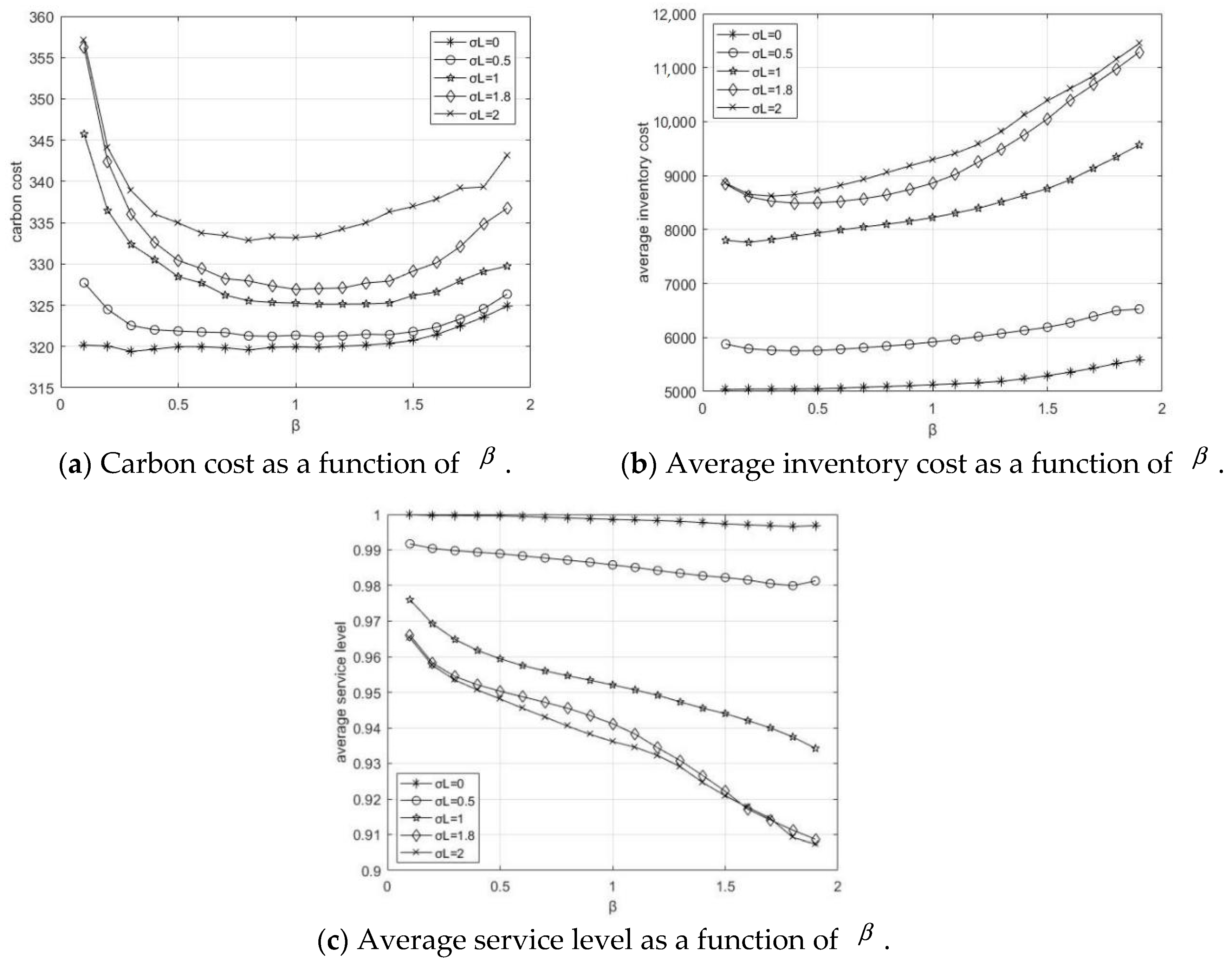
Figure 4a–c depicts carbon costs, average inventory costs, and average service levels with the system adjustment parameter
under different lead times and standard deviations
. It can be seen that the values of performance indicators change significantly with different uncertainty degree of the lead time. When the standard deviation of lead time
increases, the average inventory cost and carbon cost decreases, while the average service level increases. However, the change patterns of the three performance indicators are different. With the increase of the parameter
, the carbon cost decreases initially, and then rises smoothly. The average inventory cost is positively correlated with the parameter
, while the average service level is negatively correlated with the parameter
.
We now discuss the rate of change for each performance indicator caused by the stochastic lead times. The change rate is expressed in the form of growth rate as
and
represents the average growth rate of the three indicators in
Table 4. Overall, when the standard deviation of lead time increases, the IR of the carbon cost
and the average inventory cost
remain positive, while the average service level
remains negative. In other words, higher lead time uncertainty deteriorates the performance of the inventory system. The lead time uncertainty negatively affects
, whose average growth rate AIR reaches 17.25%, as shown in
Table 4. In addition, the effect of random lead time on
is slightly greater than that on the
, and the average growth rates are –1.62% and 1.29%, respectively.
Table 4 shows that the greater the lead time uncertainty, the greater the change rate of the performance indicators. For the carbon cost
, when the standard deviation of lead time
increases to 0.5, the growth rate IR remains 0.62%. However, when
increases from 0.5 to 2, the change rate of
for all stages remains above 1%. The IR decreases initially, and then rises. This implies that lead time uncertainty will lead to an increase in
, but the rate of cost increase will fluctuate. When the
changes from 0 to 1, average inventory cost
and average service level
rises to 39.32% and 3.38%, respectively. Then, as the fluctuation of lead time intensifies, the rates keep declining. In the transition range of 1.8–2, they fall to 2.82% and 0.23%, respectively. The results summarized in
Table 4 are consistent with what
Figure 4 shows.
5.2. Effect of Stochastic Lead Times on Order Decision
In this subsection, we focus on the relationship between stochastic lead times and inventory systems. It can be observed from
Figure 4 that when the standard deviation of lead time
increases from 0 to 0.5, the curves of carbon cost
, average inventory cost
, and average service level
remain relatively smooth, and they are least affected by the change of parameter
. In contrast, when
increases from 1 to 2, these three performance indicators change significantly. In particular, the average inventory cost
and average service level
continue to rise and fall with the increase of parameter
. However, the carbon cost curve shows a completely different trend.
Figure 4a shows that when
is small, the curve remains roughly smooth, which indicates that when the lead time is short, the parameter has little influence on carbon cost. In contrast, with an increase in
, the minimum point of the curve gradually decreases, and the decision-making area of ordering is reduced. Hence, there exists an optimal order policy to minimize carbon costs. This observation implies that lead time uncertainty influences the adjustment of ordering decisions on carbon cost.
Appendix B is a data table of a computer simulation experiment, which reveals inventory system performance indicators for different standard deviations of lead time and different
values. In comparison, the variance of
is the largest, followed by the variance of
, which is then followed by the variance of
—and this ranking is not impacted by different values of the standard deviations. Regardless of the uncertainty degree of lead time, the average inventory cost
is most affected by the parameter
, followed by
and
. However, the uncertainty level of lead time changes the strength of the adjusting function of parameter
. See
Table 5.
Table 5 depicts the values and the relative change rates of three indicators under
with the parameter
being 0.2, 0.8, and 1.8, respectively. Different values of
represent different order policies. IR1 indicates the growth rate of indicators when
changes from 0.2 to 0.8, while IR2 indicates the growth rate of indicators when
increases from 0.8 to 1.8. Again,
CC represents the carbon cost,
represents the carbon cost, represents the average inventory cost, and
represents the average service level.
Table 5 shows that when the
increases from 0.2 to 0.8 under fixed lead time,
decreases by 0.15%,
AC increases by 0.95%, while
increases by 0.07%. However, when
changes from 0.8 to 1.8,
CC increases by 1.25%,
AC increases by 8.35%, and
ASL decreases by 0.24%. Hence, it can be concluded that under fixed lead times, the policies of
β = 0.2 and
β = 0.8 have no significantly different impacts on the inventory system, but they are both better than the policy of
β = 1.8. When the standard deviation of lead time is 0.5, the conclusion is similar.
When the standard deviation of lead time increases to 1, 1.8, and 2, the impacts of the different ordering policies on the system change. When β increases from 0.2 to 0.8, CC decreases more than 3.2%, which is much larger than when . increases by more than 4.3%, except when lead time standard deviation is 1.8. The increase, then, is only 0.36%. The decreasing ASL when σL = 1, 1.8, or 2 is also greater than that of fixed lead time. Therefore, β = 0.8 is the better ordering decision criterion than β = 0.2 When parameter β changes from 0.8 to 1.8, CC and AC both increase significantly. The average inventory cost AC increases to 20%. The ASL also increases significantly from 1.80 to 3.6% when β increases. While adopting the order policy of β = 0.8, the inventory system becomes more stable, and its impact on cushioning lead time fluctuation is more efficient than that of policy β = 1.8 Overall, it can be inferred that stochastic lead times does affect the regulation of the ordering decision.
5.3. Summary of Experimental Results
Through the above experimental data analysis, we can see that:
(1) Stochastic lead times mainly affect the strength of the inventory system performance. The experimental results show that random lead time has an insignificant impact on the changing trend of each indicator. However, it greatly alters the values of the performance indicators. The sharper the lead time fluctuates, the higher the carbon cost and the average inventory cost of the system and the lower the service level. Thus, the overall performance of the inventory system decreases. The influence of lead time fluctuation on the three system performance indicators is different. Stochastic lead time significantly changes the average inventory cost, while it moderately changes the average service level. In addition, the average service level influenced by the lead time is slightly higher than the carbon cost. Furthermore, with the lead time turning to be more volatile, the inventory system performance continues to be weak, but at a slower pace.
(2) Optimizing order policy can mitigate the negative impact of stochastic lead times on the inventory system. Our simulation results show that under the same uncertainty of lead time, the impact of different ordering policies on the system’s performance is different, especially when the lead time fluctuates greatly. This phenomenon demonstrates that the inventory system is more sensitive to the order policy when lead time varies. In other words, when the lead time is volatile, the supply chain system is sensitive, and the reverse adjustment function of ordering policies is strong. Hence, there exists appropriate order decisions to weaken the negative impact of lead time fluctuation on the supply chain.
(3) The fluctuation of lead time affects the regulation effect of order decisions on an inventory system. Ordering decisions have a moderate effect on the inventory system. However, when the lead time is random, the efficiency of adjustment changes. When the lead time fluctuation is mild, the inventory system is relatively stable, and an order decision does not cause the system to oscillate dramatically. The increase in lead time randomness brings a series of management problems, such as inventory control, procurement planning, order delivery, etc. Furthermore, it puts the supply chain system in a volatile state, which lowers the anti-interference ability of the system. Then, the order decision is the decisive factor in determining the system’s performance. Moreover, the average inventory cost is mostly affected by order decisions, followed by carbon cost, and then average service level.
(4) Impacts on carbon cost are different for average inventory cost and average service level. In terms of performance indicator fluctuation with lead time variance, the value span of carbon cost is weaker than that of inventory cost and service level, but the change trend is more complex. This brings management challenges to balance the system’s performance indicators in a low-carbon economy. Furthermore, when ordering decision-making is constrained by carbon policy, the carbon cost change can be taken as the reference point, so that inventory cost and service level can be balanced to maintain a minimum carbon cost.
6. Conclusions
Based on the APVIOBPCS model, this paper constructs a three-stage supply chain with the distributors as the focal firm in a periodic continuous review system. The traditional APVIOBPCS model primarily focuses on the impact of parameters of adjustment for inventory and work-in-process inventory discrepancy on supply chains under fixed lead time. However, in business practice, it is difficult to achieve a fixed lead time. Therefore, this paper makes an important contribution by introducing stochastic lead times into the basic APVIOBPCS model.
Our results show that stochastic lead time only affects the values, but not the trends of the inventory system performance indicators. Furthermore, the three performance indicators have different trends under different order policies. The negative impact of stochastic lead times can be dampened by the appropriate order policy. Moreover, the carbon cost curve is concave with regard to the order policy, while the inventory cost curve is continuously increasing, and service level curve is decreasing. Hence, when the managers make order decisions, they can take carbon cost change as reference point, and then balance inventory cost and service level to maintain a minimum carbon cost.
Carbon emission policies in many countries are still in the exploratory stage. In future studies, the optimal carbon emission policy may be identified. Future study can also focus on the interactions between carbon regulation policies and supply chain conditions, so that appropriate policies can be formulated to achieve green sustainable development.


