Evaluating the Sustainable Use of Saline Water Irrigation on Soil Water-Salt Content and Grain Yield under Subsurface Drainage Condition

Abstract

A sustainable irrigation system is known to improve the farmland soil water-salt environment and increase crop yields. However, the sustainable use of saline irrigation water under proper drainage measures still needs further study. In this study, a two-year experiment was performed to assess the sustainable effects of saline water irrigation under subsurface drainage condition. A coupled model consisting of the HYDRUS-2D model and EPIC module was used to investigate the effects of irrigation water salinity (IWS) and subsurface drainage depth (SDD) on soil water-salt content and summer maize yield when saline water was adopted for irrigation under different subsurface drainage measures. Summer maize in the two-year experiments were irrigated with saline water of three different salinity levels (0.78, 3.75, and 6.25 dS m⁻¹) under three different drainage conditions (no subsurface drainage, drain depth of 80 cm, and drain depth of 120 cm). The field observed data such as soil water content, soil salinity within root zone, ET and grain yield in 2016 and 2017 were used for calibration and validation, respectively. The calibration and validation results indicated that there was good correlation between the field measured data and the HYDRUS-EPIC model simulated data, where RMSE, NSE (> 0.50), and R² (> 0.70) satisfied the requirements of model accuracy. Based on a seven × seven (IWS × SDD) scenario simulation, the effects of IWS and SDD on summer maize relative grain yield and water use efficiency (WUE) were evaluated in the form of a contour map; the relative grain yield and WUE obtained peak values when drain depth was around 100 cm, where the relative yield of summer maize was about 0.82 and 0.53 at IWS of 8 and 12 dS m⁻¹, and the mean WUE was 1.66 kg m⁻³. The proper IWS under subsurface drainage systems was also optimized by the scenario simulation results; the summer maize relative yield was still about 0.80 even when the IWS was as high as 8.61 dS m⁻¹. In summary, subsurface drainage measures may provide important support for the sustainable utilization of saline water in irrigation. Moreover, the coupled HYDRUS-EPIC model should be a beneficial tool to evaluate future sustainability of the irrigation system.

1. Introduction

The lack of fresh-water resources for agricultural irrigation is limiting the sustainable development of agriculture worldwide. In recent years, as a supplemental irrigation water source, saline water has been widely utilized in fresh water-deficient areas. Previous researches have reported that saline water irrigation is acceptable for moderate and mild salt-tolerant crops [1,2,3]. The response mechanism of soil salinity and crop yield to saline water irrigation has been studied extensively. However, the strategy to eliminate soil salts added by saline water still need further study [4,5]. Verma et al. confirmed that the salt accumulated in soil profile may lead to the risk of soil salinization [6]. Similar research also found that the decrease of water available for plant root extraction was mainly due to the increase of soil salinity [7,8]. Therefore, in order to ameliorate the soil environment and keep healthy crop growth, appropriate field management practices, including field drainage, and selection of appropriate irrigation water salinity are essential when saline water is utilized for irrigation.

As a subterranean land drainage technology, subsurface drainage was traditionally used for field groundwater management [9,10,11]. Sharma and Feng both proposed that subsurface drainage could provide great potential for saline water irrigation [12,13]. Extensive research showed that subsurface drainage depth (SDD) was a main factor that affects drainage capacity [14,15]. However, the appropriate drainage depth varies with the change of soil properties and groundwater conditions, it is still in dispute about the appropriate depth [16,17]. Thus, more research is essential to determine the proper drain depth and reveal the effects of subsurface drainage depth on soil water-salt and grain yield, especially in saline water irrigation system [18].

Relying on field experiments alone to determine the proper water management strategies and drainage practices might be incomplete and time-consuming [19]. The HYDRUS model has been adopted in various soil water-salt studies. The model can simulate two- or three-dimensional water and solute transport processes in subsurface drainage systems with its various boundary conditions and sophisticated, graphical, user-friendly interface [20,21,22,23,24,25,26,27,28]. Since the crop growth response was not considered in the original version of HYDRUS-2D, this model was usually coupled with other crop growth modules such as EPIC, and SWAP to study both the hydrologic and crop growth processes [29]. Among the crop growth modules, EPIC has been a priority used model in crop growth and yield simulation due to a relatively less data input requirement and abundant crop variety options [30,31]. Simulation results by Wang, et al., Han et al. and Wang et al. suggested that the coupled HYDRUS-EPIC model could be used in studying the effects of different agronomic measures such as sprinkler irrigation, saline water irrigation on soil water, solute transport, ET, and grain yield [32,33,34]. Previous studies using the model have focused more on the effects of irrigation methods, irrigation amount and water salinity on soil water-salt dynamic, grain yield and water use efficiency in different regions worldwide, and the relationships between irrigation and grain yield has been established under various irrigation systems [35,36]. While under drainage condition, especially in subsurface drainage condition, the knowledge of the saline water irrigation still needs further study [37,38]. Together with the field experiment and coupled model, the sustainable effects of saline water irrigation under subsurface drainage condition would be systematically evaluated in various irrigation and drainage scenarios [39,40].

The field and model experiment conducted in this research were: (1) To evaluate the accuracy of the HYDRUS-EPIC model by field experiment data and simulation data; (2) to evaluate the effects of IWS and SDD on summer maize relative yield and WUE by scenario simulation; (3) to determine proper irrigation water salinity under subsurface drainage conditions.

2. Materials and Methods

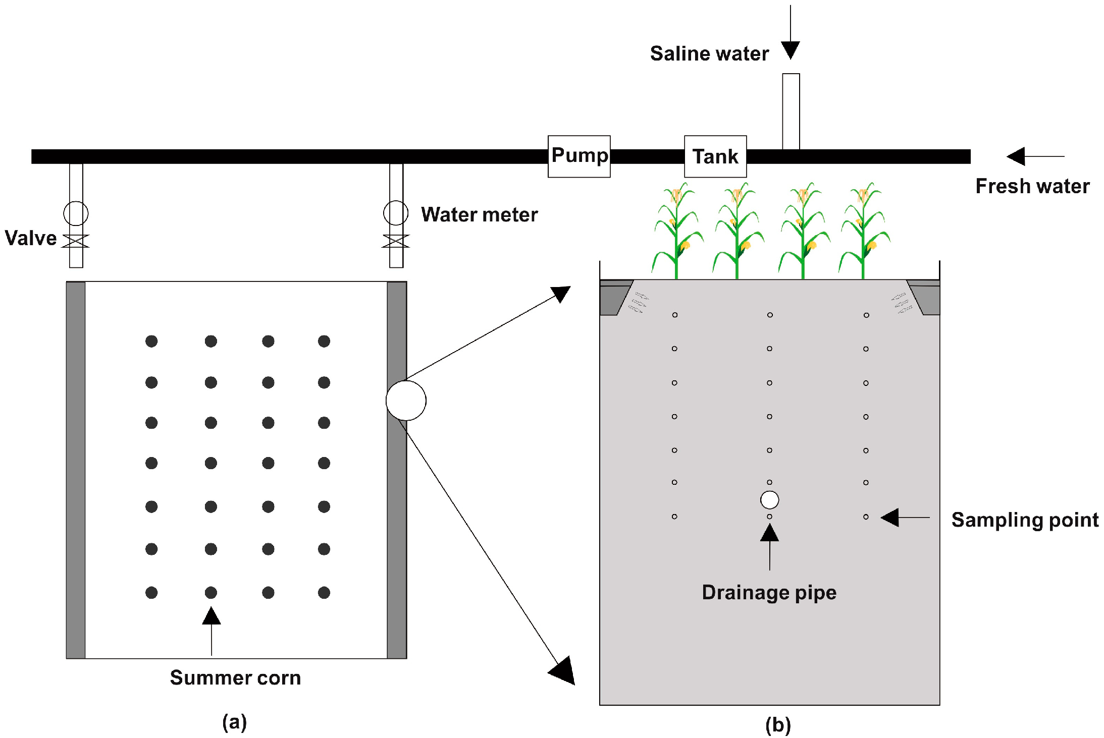
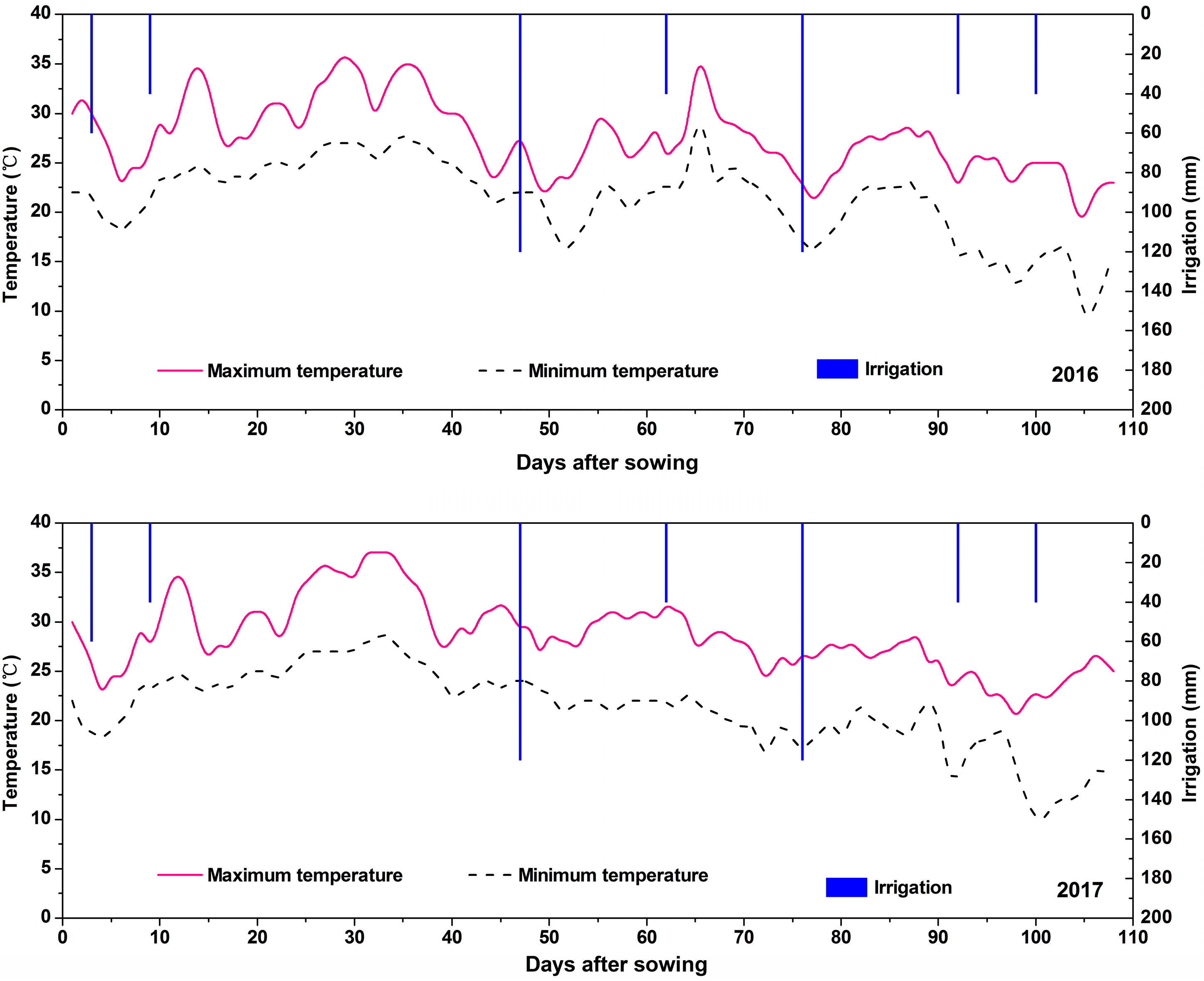
2.1. Field Experiments

A two-year experiment was performed in lysimeters during the year of 2016 and 2017 at the Key Laboratory of Efficient Irrigation-Drainage and Agricultural Soil-Water Environment in Nanjing, China (118°60′E, 31°86′N). The mean annual temperature in the experiment area was 15.7 °C, and the mean annual rainfall and evaporation were 1021.3 and 2000 mm, respectively. The summer maize (Longping-206) in this study were irrigated with saline water in three concentration gradients (S1: 0.78, S2: 3.75, and S3: 6.25 dS m⁻¹) under three different drainage conditions (D0: no subsurface drainage, D1: drain depth of 80 cm, and D2: drain depth of 120 cm) in three replicates. Summer maize was sown in mid-June (20 June 2016 and 18 June 20 2017) with the row spacing and plant spacing of 40 cm × 40 cm. The fertilizer application amount was similar to the study by Feng [13]. A total of 225 kg ha⁻¹ was applied as base before sowing in the form of ammonium nitrate where P2O5 and K2O at a rate of (N:P2O5:K2O = 28%:6%:6%). Urea was applied at a rate of 300 kg ha⁻¹ with the first irrigation water in all treatments during the maize reviving stage. Moreover, the design of the lysimeters was similar to the ones used in Feng’s study as shown in Figure 1, where the lysimeters were approximately 15 m³ (2.5 × 2 × 3 m). There were all together 27 lysimeters adopted in this study.

The soil physical properties for different layers (0~20, 20~40, 40~80, and 80~120 cm) in the lysimeters are listed in

Table 1. Soil physical properties for layered depth.

Soil Depth (cm)	Soil Particle Percent (%)			Soil Bulk Density (g cm−3)	Field Capacity (cm3 cm−3)
	Sand (2.0~0.02 mm)	Silt (0.02~0.002 m)	Clay (<0.002 mm)
0~20	43.91	36.41	19.68	1.33	0.38
20~40	42.59	37.28	20.13	1.41	0.37
40~80	41.34	36.68	21.98	1.46	0.35
80~120	40.25	38.12	21.63	1.48	0.23

. The soil particle percent, soil bulk density, and field capacity were used for estimating initial values of soil hydraulic parameters according to van-Genuchten’s model [41]. The estimated soil hydraulic parameters are shown in

Table 2. Initial and calibrated values of soil hydraulic parameters for different soil layers.

Soil Depth (cm)	θr (cm3 cm−3)	θs (cm3 cm−3)	α (cm−1)	n	Ks (mm d−1)
Initial values
0~20	0.096	0.483	0.014	1.375	149.70
20~40	0.092	0.458	0.013	1.377	93.30
40~80	0.089	0.441	0.013	1.372	71.20
80~120	0.088	0.434	0.013	1.350	62.10
Calibrated values
0~20	0.096	0.483	0.015	1.200	149.71
20~40	0.092	0.458	0.012	1.200	93.32
40~80	0.089	0.441	0.010	1.180	71.24
80~120	0.088	0.434	0.012	1.252	62.12

.

Irrigation water controlled by a water meter was applied to each lysimeter by furrow irrigation. During the summer maize growing seasons in 2016 and 2017, a total of 460 mm irrigation water was applied to each lysimeter in seven irrigation events. Fresh water with irrigation amounts of 60 mm was applied at sowing. In the critical growth periods of the summer maize such as the tasseling and filling stage, two irrigation events with a total irrigation amounts of 120 mm were applied for soil salt leaching. For the other four irrigation events, all irrigation amounts were 40 mm at 10, 62, 92, and 100 days after sowing. The two-year experiments were carried out under a rain shelter. Meteorological data were recorded by an automated weather station located at the experiment field. The maximum air temperature, minimum air temperature, and the irrigation amounts are shown in Figure 2.

Soil samples were obtained using a 4 cm auger from soil depths of 20, 40, 60, 80, 100, and 120 cm in each lysimeter, and the sampling interval was 15 days during the summer maize growth period in both 2016 and 2017. The soil water contents were determined using the gravimetric method. EC_1:5 (dS m⁻¹), which is the electrical conductivity of a soil and water mixture in the ratio 1:5 by mass, was determined using an electrical conductivity meter. The EC_1:5 was then converted to the EC_e (dS m⁻¹), which is the electrical conductivity of the saturated paste according to Equation (1) obtained in the laboratory experiment by Feng with R² = 0.994 [13].

$$E{C}_e=14.77{\mathrm{EC}}_{1:5}-0.225$$

(1)

2.2. Model Experiments

The hydrologic module in HYDRUS model was coupled by the crop growth module in EPIC in this study. The crop growth module of EPIC was preferred at field production level due to its less demanding data input requirement, which used a unified approach to simulate more than 100 types of crops [42]. The data exchange between the HYDRUS and EPIC models took “day” as the time step. The coupling model used the hydrologic model in HYDRUS to simulate the soil water and salt dynamics and the effect of soil water-salt on the root water absorption. Then, the results were output to the EPIC crop growth module to analyze the crop growth. The EPIC model was used to simulate and calculate the crop growth indicators, and the results were fed back to the hydrologic model in HYDRUS to further simulate and analyze the soil water and salt transport. The model was encoded by FORTRAN 90 based on Microsoft Windows system with the actual evaporation and transpiration rates as upper boundary condition and subsurface drainage as the bottom boundary condition. The Penman–Monteith equation was used for the estimate of ET_p and crop parameters, where the crop parameters adopted in this study was 1.45 [42,43].

2.2.1. Root Water Uptake

The root water absorption was calculated according to Feddes model as follows [44,45,46,47,48]:

$$S(h,h_{\varphi },z,t)=\alpha (h,h_{\varphi },z,t)\times b(z)\times T_p$$

(2)

where S(h, h_ϕ, z, t) is the root water absorption, α(h, h_ϕ, z, t) is the stress response function, b(z) is the distribution of water uptake, mm⁻¹, and T_p is the potential crop transpiration, mm d⁻¹.

The actual transpiration rate T_a was calculated by the following equation:

$$T_a=T_p{\displaystyle {\int }_0^L\alpha }(h,h_{\varphi })b(z)dz$$

(3)

where L is the root depth, cm, which was calculated as:

$$L_i=2.5L_{\max }(HU{I}_i) L_{\mathrm{i}}\le L_{\max }$$

(4)

$$L_i=L_{\max } \hspace{0.17em}\hspace{0.17em}\hspace{0.17em}\hspace{0.17em}{L}_{\mathrm{i}}>L_{\max }$$

(5)

where L_max is the maximum root depth, which was 80 cm in this study, and HUI is the heat unit coefficient of crop [42]. The root water uptake reduction factors are list in

Table 3. Initial and calibrated values of water and salt stress function.

Parameters (mm)	Description	Initial Values	Calibrated Values
h1	h when root can absorb water from soil (mm)	−150	−180
h2	h when root water absorption is not affected (mm)	−300	−320
h3h	h when WUR starts at high demand (mm)	−3250	−3500
h3l	h when WUR starts at low demand (mm)	−6000	−6400
h4	h when WUE = 0 (mm)	−80,000	−85,000
h50%	h when WUR = 50% caused by salt stress (mm)	−50,000	−55,000
Th	Higher threshold of atmospheric evaporation capacity (mm d−1)	5	5
Tl	Lower threshold of atmospheric evaporation capacity (mm d−1)	1	1

Note: In this table, WUR refers to water uptake reduction.

.

2.2.2. Soil Solute Transport Module

The HYDRUS model uses convection dispersion equation to express soil solute transport process as follows:

$$\frac{\partial (\theta c+\rho s)}{\partial t}=\frac{\partial }{\partial z}(\theta D\frac{\partial c}{\partial z})-\frac{\partial qc}{\partial z}$$

(6)

where c is the concentration of solute in soil solution, dS m⁻¹, ρ is the dry bulk density of soil, g cm⁻³, s is the concentration of solute adsorbed on soil particles, q is the Darcy velocity in direction, mm d⁻¹, and D is the hydrodynamic dispersion coefficient of saturated unsaturated soil, mm² d⁻¹.

2.2.3. Crop Growth Module

Generally, the harvest index value of most crops is relatively stable under stable environment and water and salt conditions [42]. Therefore, the model migrates the harvest index to calculate crop yield:

$$YLD=HI{B}_a$$

(7)

where YLD represents the crop yield, kg ha⁻¹, B_a represents the aboveground biomass of the crop, kg ha⁻¹, and HI represents the harvest index of the crop, which was 0.45 in our study.

Aboveground biomass is affected by solar radiation, while solar radiation is closely related to the leaf area. Beer’s law offers a calculation method as follows [45]:

$$\mathsf{\Delta }B=(BE)\times 0.5(RA)[1-\exp (-0.65LAI)]$$

(8)

where ΔB is the potential increase in biomass, kg ha⁻¹, BE is the ability of crop convert solar energy into biomass, which was 25 (kg ha⁻¹) in the present study, RA is solar radiation, MJ m⁻², and LAI is the leaf area index [46,47].

2.2.4. Model Calibration and Validation

The measured and predicted soil water-salt content and crop grain yield of 2016 and 2017 were used to calibrate and validate the coupled model, respectively. The soil hydraulic and parameters and root water uptake and crop growth parameters were the main parameters calibrated and validated in this study. In our research, θ_s and K_s were based on laboratory measurement, and θ_r, n, a and root water uptake were the main calibration parameters since they were much more sensitive than θ_s and K_s in the model operation process [31]. The initial input soil hydraulic parameters were predicted by van-Genuchten’s model [41], and then calibrated and validated by the measured and predicted soil water content in 2016 and 2017, respectively. The root water uptake calculated according to Feddes model was calibrated and validated by the measured and predicted soil water-salt content in 2016 and 2017, respectively [44]. The initial crop growth parameters were estimated from the default values of the EPIC model [42], and then calibrated and validated by the measured and predicted grain yield data in 2016 and 2017, respectively.

2.2.5. Scenario Analysis

After calibration and validation, the coupled model was used to predict summer maize yield and water use efficiency (WUE) under different irrigation water salinity and drainage conditions. A total 49 simulation scenarios consisting of seven levels of irrigation water salinity (0, 2, 4, 6, 8, 10, and 12 dS m⁻¹) and seven levels of subsurface drain depth (no subsurface drain, 60, 80, 100, 120, 140, and 160 cm) were run with the validated coupled model. The input parameters such as soil physical properties, soil hydraulic parameters, and water uptake parameters were the same as the field experiment, and the daily meteorological data of 2016 were selected for the scenario simulation. To determine the effects of irrigation water salinity on relative grain yield and WUE under different drainage conditions, the polynomial regression method was used to fit the simulation results. Finally, the proper irrigation water salinity was optimized based on the established relationships between grain relative yield and IWS under different drainage conditions.

2.3. Statistical Analysis

The field observed soil water contents, soil salinities, ET, and grain yield obtained in 2016 and 2017 were used for calibrating and validating the coupled HYDRUS-EPIC model, respectively. The parameters root mean square error (RMSE), determination coefficient (R²), and Nash–Sutcliffe efficiency (NSE) were adopted for evaluating model accuracy:

$$RMSE=\sqrt{\frac{1}{N}{\displaystyle {\sum }_{i=1}^N{(P_i-O_i)}^2}}$$

(9)

$$R^2=\frac{{\displaystyle {\sum }_{i=1}^N(O_i-O_a)(P_i-P_a)}}{\sqrt{{\displaystyle {\sum }_{i=1}^N{(O_i-O_a)}^2}}\sqrt{{\displaystyle {\sum }_{i=1}^N{(P_i-P_a)}^2}}}$$

(10)

$$NSE=1-\frac{{\displaystyle {\sum }_{i=1}^N{(P_i-O_i)}^2}}{{\displaystyle {\sum }_{i=1}^N{(O_i-O_a)}^2}}$$

(11)

where RMSE is the root mean square error; R² is the determination coefficient; NSE is the Nash– Sutcliffe efficiency; O_i is the observed value from the field experiment; P_i is the predicted value from the model simulation; O_a is the average of the observed value from the field experiment; P_a is the average of the model simulation values. In general, the NSE ranges from −∞ to 1. This value is close to 1, which is better model performance. R² ranges from 0 to 1, and RMSE values close to zero and R² close to 1 indicate good model performance.

3. Results

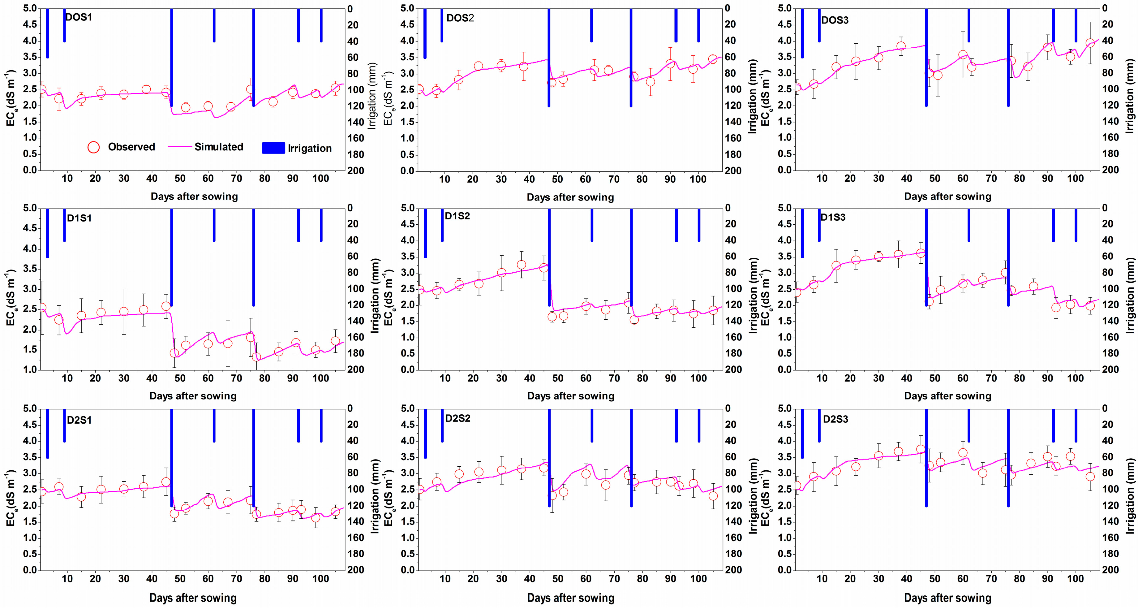
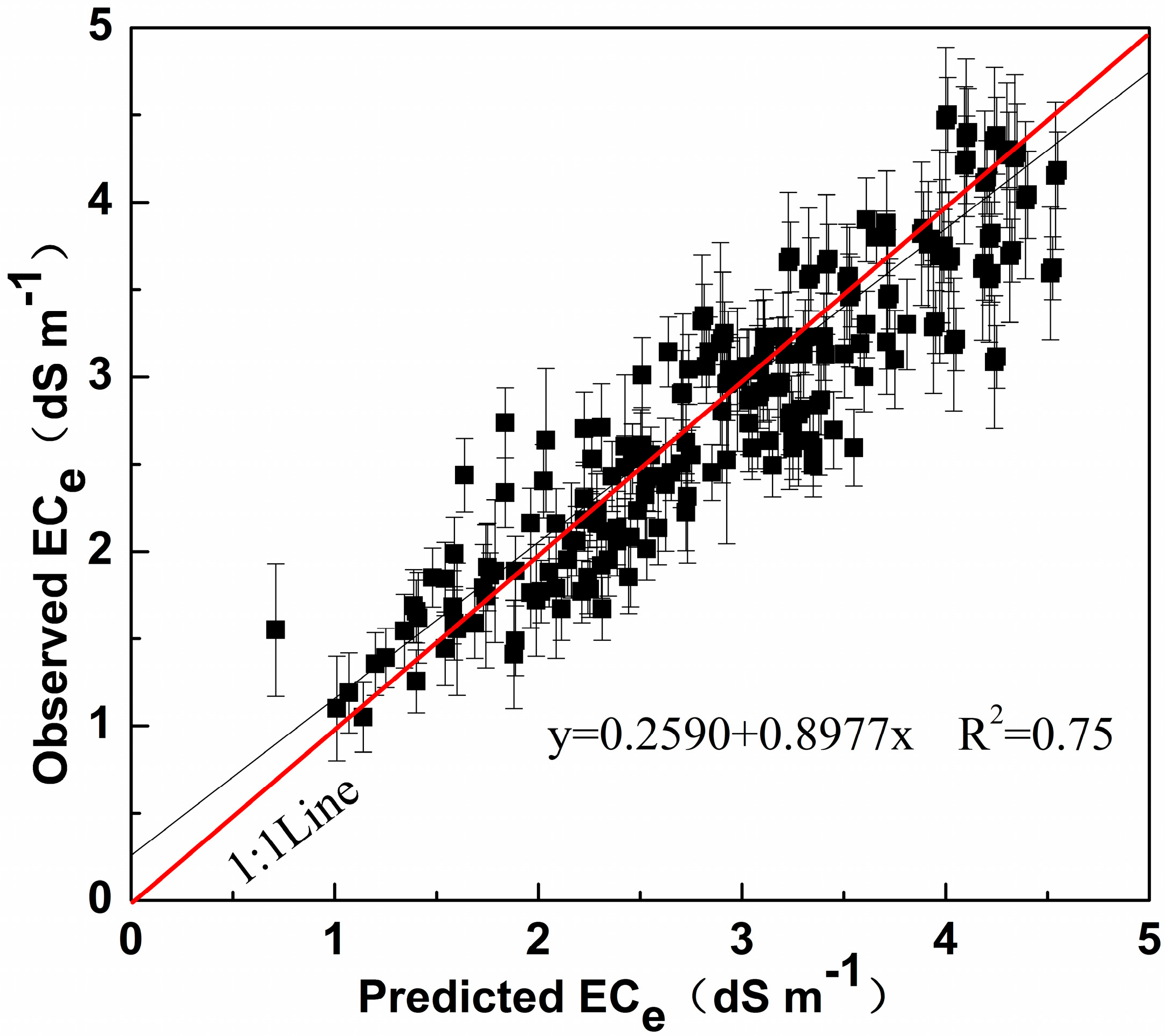
3.1. Model Calibration and Validation

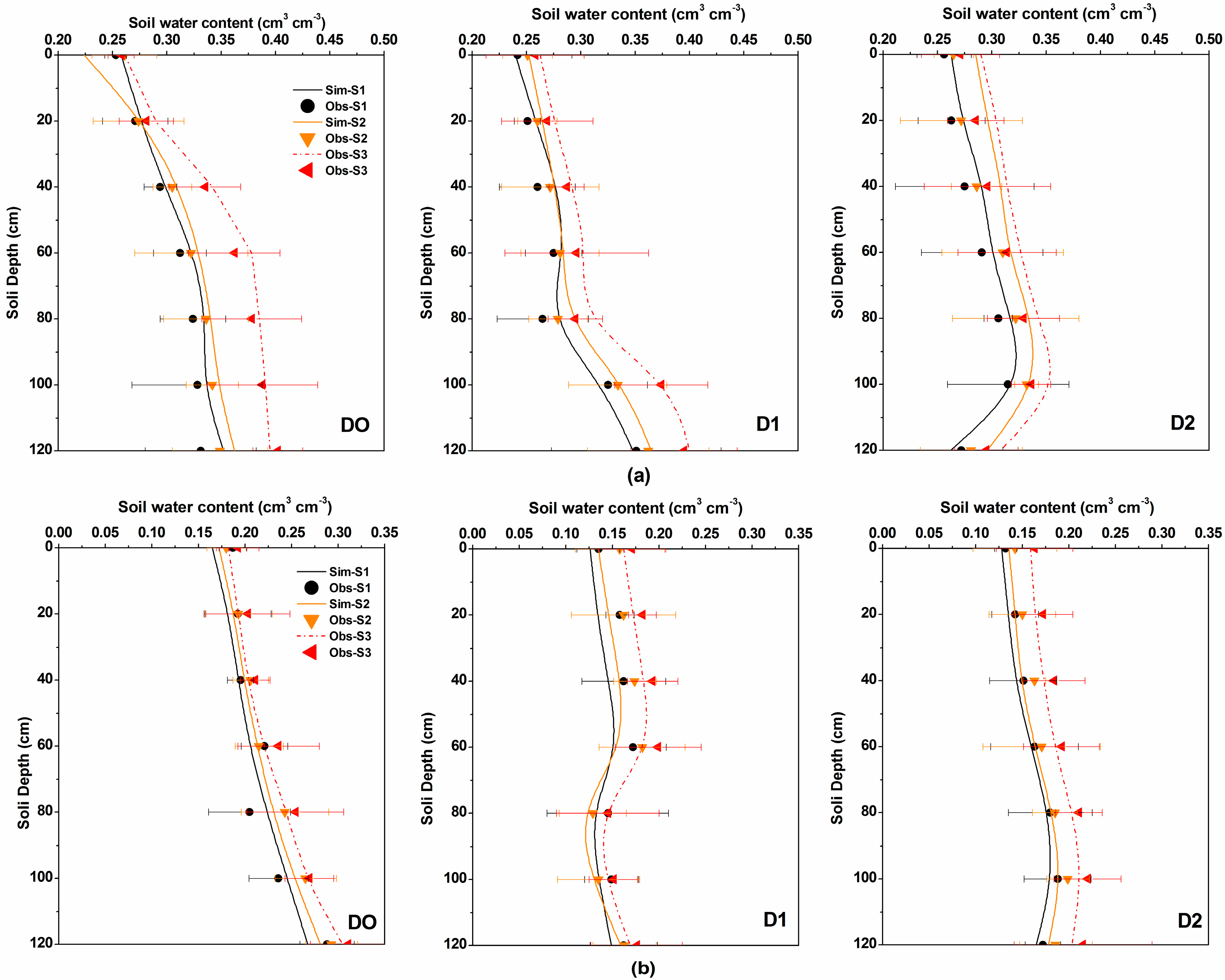
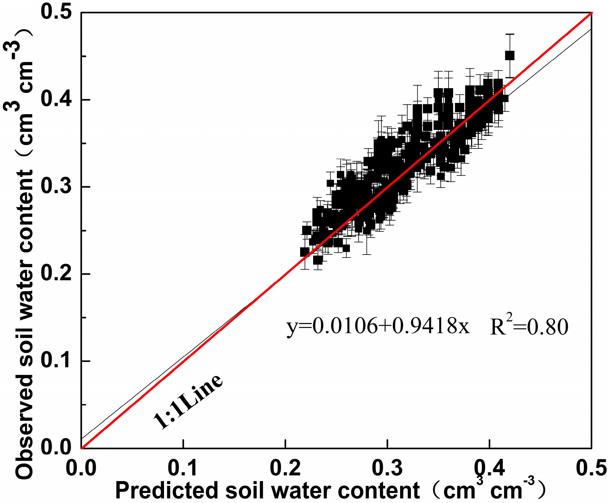
3.1.1. Soil Water Contents

As shown in Figure 3a,b, field observed soil water contents within the soil depth 0~120 cm at the time of sowing (Figure 3a) and harvest (Figure 3b) in 2016 (calibration period) were compared with the simulated values. In our study, soil water content under high IWS was higher than that under low IWS in different drainage conditions. Moreover, the soil water contents were low at the drain depth since the subsurface drainage system provided an unobstructed drainage path. The differences between observed and predicted soil water contents at sowing time and harvest time were apparent during the calibration periods. The soil water content at harvest time was lower than that at sowing time. The main reason for this phenomenon was that the field was relatively dry at harvest and the average soil water content much lower. Therefore, the range of soil water content at harvest time was smaller than that at sowing time. However, the trend of soil water content at harvest time was similar to that at sowing time, i.e., it decreased with proximity to the drain depth. In D0, D1, and D2 at sowing time and harvest time, the experimental data and simulation data showed good correlation after calibration as shown in Figure 3. The model accuracy evaluating parameters shown in

Table 4. Model accuracy evaluation for soil water-salt dynamics in 2016 and 2017.

Year·	Drain Depth (cm)	Soil Water Content (cm3cm−3)			ECe (dS m−1)
		RMSE	NSE	R2	RMSE	NSE	R2
2016 (Calibration)	D0 (no drain)	0.03	0.61	0.75	0.28	0.68	0.83
	D1(80)	0.02	0.63	0.79	0.39	0.51	0.71
	D2 (120)	0.02	0.71	0.85	0.29	0.58	0.75
2017 (Validation)	D0 (no drain)	0.03	0.63	0.71	0.31	0.66	0.85
	D1 (80)	0.03	0.68	0.80	0.48	0.51	0.65
	D2 (120)	0.02	0.75	0.88	0.35	0.54	0.75

indicated that, after calibration RMSE ranged from 0.02 to 0.05 cm³ cm⁻³, NSE ranged from 0.61 to 0.75, and R² ranged from 0.68 to 0.85. As shown in Figure 4, during validation (2017), the experimental data and simulation data also show good correlation relationship, since both were distributed near the 1:1 line. As shown in Table 4, RMSE during validation ranged from 0.01 to 0.03 cm³ cm⁻³, NSE ranged from 0.63 to 0.75, and R² ranged from 0.71 to 0.88, and the floating range of these parameters were similar compared with other studies [31,49]. By comparing the observed and predicted soil water content data shown in Figure 3 and Figure 4 and evaluating the model accuracy parameters listed in Table 4, it was generally believed that the soil hydraulic parameters in Table 2 were acceptable for the coupled model. Thus, we confirmed that the simulation effect was satisfactory in soil water content simulation under HYDRUS-EPIC model.

3.1.2. Soil Salinity

Figure 5 shows a comparison between the field observed soil salinity data and the simulated data within the root zone depth in 2016 (calibration period). Compared to D0 treatment, the increase of EC_e was slight for S1 (1.95~2.55 dS m⁻¹), and more striking for S2 (2.48~3.45 dS m⁻¹) and S3 (2.58~3.95 dS m⁻¹). The reason for this phenomenon is that there was no drainage under this treatment, therefore the soil salinity in S2 and S3 fluctuated with irrigation according to the irrigation water salinity. At the drain depths of 80 cm (D1) and 120cm (D2), similar EC_e dynamics are observed shared with the three levels of IWS (S1, S2, and S3), where EC_e increased with increasing IWS. Moreover, EC_e was lower when SDD was 80 cm (D1) than when it was 120 cm (D2).

In D0, D1, and D2 treatments, the experimental data and simulation data showed good correlation during calibration, as shown in Figure 5. The model evaluating parameters shown in Table 4 also indicated that RMSE during calibration (2016) ranged from 0.28 to 0.39 dS m⁻¹, NSE ranged from 0.51to 0.68, and R² ranged from 0.71 to 0.83. As shown in Figure 6, during validation (2017), the experimental data and simulation data also incarnated great correlation relationship, since both forms of data were distributed near the 1:1 line. As shown in Table 4, RMSE in the validation period ranged from 0.31 to 0.48 dS m⁻¹, NSE ranged from 0.51 to 0.66, and R² ranged from 0.65 to 0.85. In this research, the NSE and R² values for D1 and D2 were lower than that for D0 in the simulation soil salinity. Similar simulation results were obtained by Ren et al. who obtained R² values in the range of 0.65–0.91 [50]. By comparing the observed and predicted soil salinity data shown in Figure 5 and Figure 6 and evaluating the model accuracy parameters listed in Table 4, it was generally believed that the soil hydraulic parameters in Table 2 and water-salt stress function in Table 3 were acceptable for the coupled model. Thus, we confirmed that the simulation effect was satisfactory in soil salinity simulation under HYDRUS-EPIC model.

3.1.3. ET and Crop Yield

As shown in

Table 5. Simulated and observed summer maize evapotranspiration, yields.

Yea·	Treatments	Evapotranspiration (mm)					Grain Yields (kg ha−1)
		Observed	Simulated	RMSE	NSE	R2	Observed	Simulated	RMSE	NSE	R2
2016 (Calibration)	D0S1	513 ± 12.8	502.5	7.65	0.95	0.98	7123 ± 205	7342.3	255.71	0.85	0.97
	D0S2	488 ± 15.2	479.8				6223 ± 156	5823.5
	D0S3	463 ± 11.0	462.2				5745 ± 134	5615.6
	D1S1	425 ± 13.2	435.6				7911 ± 336	7854.8
	D1S2	405 ± 5.3	400.2				7358 ± 105	7156.5
	D1S3	399 ± 10.1	398.4				6899 ± 126	6715.8
	D2S1	458 ± 13.6	466.6				7563 ± 121	7236.4
	D2S2	447 ± 11.5	455.5				6626 ± 213	6328.3
	D2S3	440 ± 11.2	448.2				6218 ± 212	5915.6
2017 (Validation)	D0S1	493 ± 12.8	495.6	11.30	0.92	0.97	7224 ± 115	7412.9	212.21	0.87	0.94
	D0S2	471 ± 12.1	482.3				6188 ± 186	6434.6
	D0S3	460 ± 13.0	472.6				5442 ± 120	5052.5
	D1S1	400 ± 10.3	409.3				8325 ± 163	8115.3
	D1S2	392 ± 13.4	395.6				7702 ± 158	7552.5
	D1S3	385 ± 12.8	392.2				7236 ± 136	7455.8
	D2S1	483 ± 19.9	492.5				7725 ± 110	7913.5
	D2S2	472 ± 20.6	480.6				6842 ± 150	6782.1
	D2S3	447 ± 16.2	449.9				6326 ± 158	6383.8

, the measured ET values were generally lower than the predicted ET values, but the experimental data and simulation data showed good correlation during calibration (2016). During calibration, the RMSE, NSE, and R² were 7.65 mm, 0.95 and 0.98, respectively (Table 5), while during validation (2017), the RMSE, NSE, and R² were 11.30 mm, 0.92 and 0.97, respectively (Table 5). As shown in Table 5, the measured grain yield values were generally lower than the predicted grain yield values in both 2016 and 2017 growing seasons. The grain yield decreased with increasing irrigation water salinity under the same drainage conditions. Moreover, the mean grain yield for D1 (drain depth: 80 cm) was obviously higher than that for D0 (no subsurface drainage) and D2 (drain depth: 120 cm) under the same irrigation water salinity. The highest ET values were obtained in D0S1 in both by observed and by simulation in 2016 and 2017 growing seasons. The ET values were obtained by calculating the water balance process in both the field experiments and the HYDRUS model. For treatments D1 and D2, discharge in the water balance was excluded by subsurface drainage effects, and thus the ET values for D0 were higher than for D1 and D2. Furthermore, the highest grain yield values were obtained in D1S1 by both observed and by simulation in 2016 and 2017 growing seasons. As was discussed above, the IWS of 0.25 dS m⁻¹ (S1) introduced the least amount of salt in the soil profile which minimized salt stress on the crop compared with IWS of 3.75 (S2) and 6.25 dS m⁻¹ (S3). Moreover, the drainage depth D1 better reduced the salt content within the crop root zone compared to drainage depth of D0 and D2. During calibration (2016), the RMSE, NSE, and R² for grain yield simulation were 255.71 kg ha⁻¹, 0.85, and 0.98, respectively (Table 5), while during validation (2017), the RMSE, NSE, and R² were 212.21 kg ha⁻¹, 0.87, and 0.94, respectively (Table 5). Similar research have evaluated winter wheat growth and yield in the Loess Plateau of China using the EPIC model [51,52]. Based on Table 5, ET and grain yield simulation by the HYDRUS-EPIC model was deemed satisfactory.

3.2. Effects on Relative Grain Yield and WUE

A contour map of the relative grain yield in each simulation scenario was generated as shown in Figure 7. When there is no subsurface drainage system, the relative yield of summer maize is about 0.5 at IWS of 8 dS m⁻¹. Additionally, when IWS was 12 dS m⁻¹, the relative yield of summer maize is 0, which means that summer maize cannot survive. Under drain depth of 100 cm, the relative yield of summer maize is about 0.82 at IWS of 8 dS m⁻¹. While at IWS of 12 dS m⁻¹, the relative yield of summer maize is 0.53, which was much higher than that under no subsurface drainage system. Under drain depth of 160 cm, the relative yield of summer maize is about 0.53 at IWS of 8 dS m⁻¹. While at IWS of 12 dS m⁻¹, the relative yield of summer maize is just 0.23, which is much lower than that under SDD of 100 cm. The results above indicated that grain yield reduction could be effectively restrained by proper arrangement of subsurface drainage system even under saline water irrigation of high concentration. Figure 7 also reflects that the relative grain yield increases initially and then decreases with the increase of SDD under all levels of IWS. In this study, the relative grain yields obtained peak values when drain depth was around 90~100 cm.

The ET in each scenario was also simulated with the coupled HYDRUS-EPIC model, and the polynomial regression method was used to fit the calculated WUE, and then the contour map of the WUE in each simulation scenario was generated as shown in Figure 8. As shown in Figure 8, the WUE decreased with increasing IWS. The highest WUE was obtained in the scenario with SDD of 100 cm, and IWS of 0 dS m⁻¹, where the WUE reached 2.08 kg m⁻³. The lowest WUE was obtained in scenario with no subsurface drainage, and the IWS of 12 dS m⁻¹, where the WUE was 0 kg m⁻³, since the relative grain yield was 0 in this scenario. From the overall perspective of Figure 8, with a constant subsurface drainage condition, the highest mean WUE was realized in scenarios where IWS was 0 dS m⁻¹, and the mean WUE was 1.64 kg m⁻³. Additionally, the lowest mean WUE was realized in scenarios where IWS was 12 dS m⁻¹, and the mean WUE was 0.55 kg m⁻³. Figure 8 also indicated that, with the increase of SDD, the WUE increased first and then decreased at the SDD of 100 cm. The mean WUE for SDD of 100 cm was 1.66 kg m⁻³. The lowest mean WUE was in the scenarios where there was no subsurface drainage condition, and the value was just 0.88 kg m⁻³. Consequently, both the IWS and SDD were the main factors that affected the crop yield and water use efficiency of summer maize.

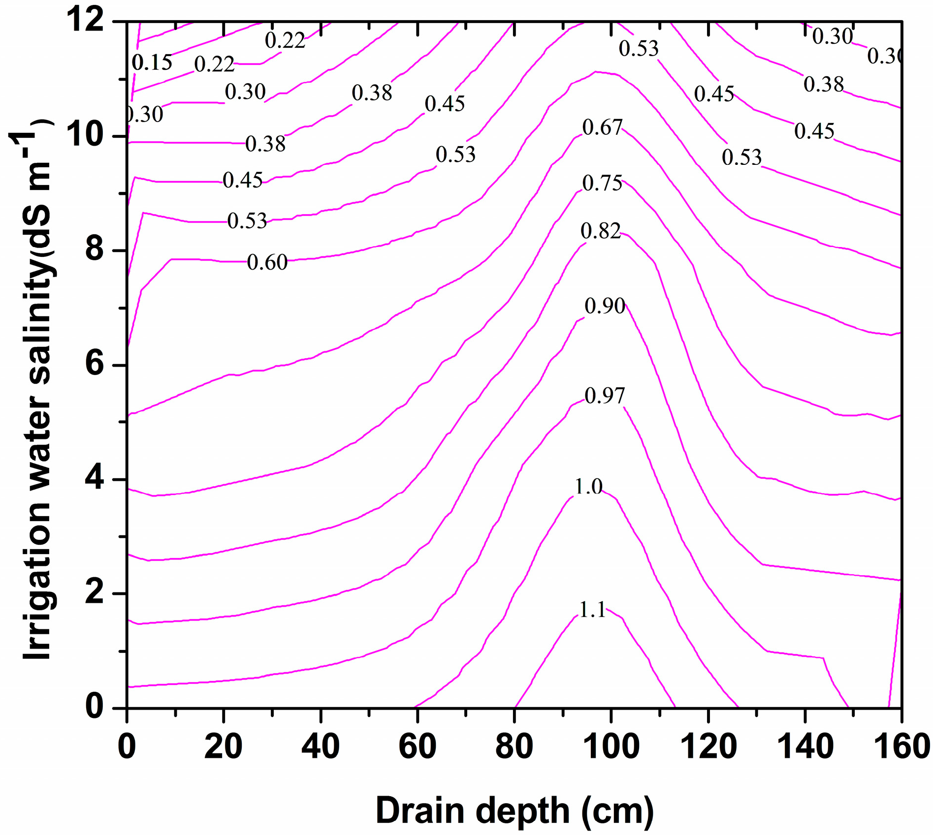
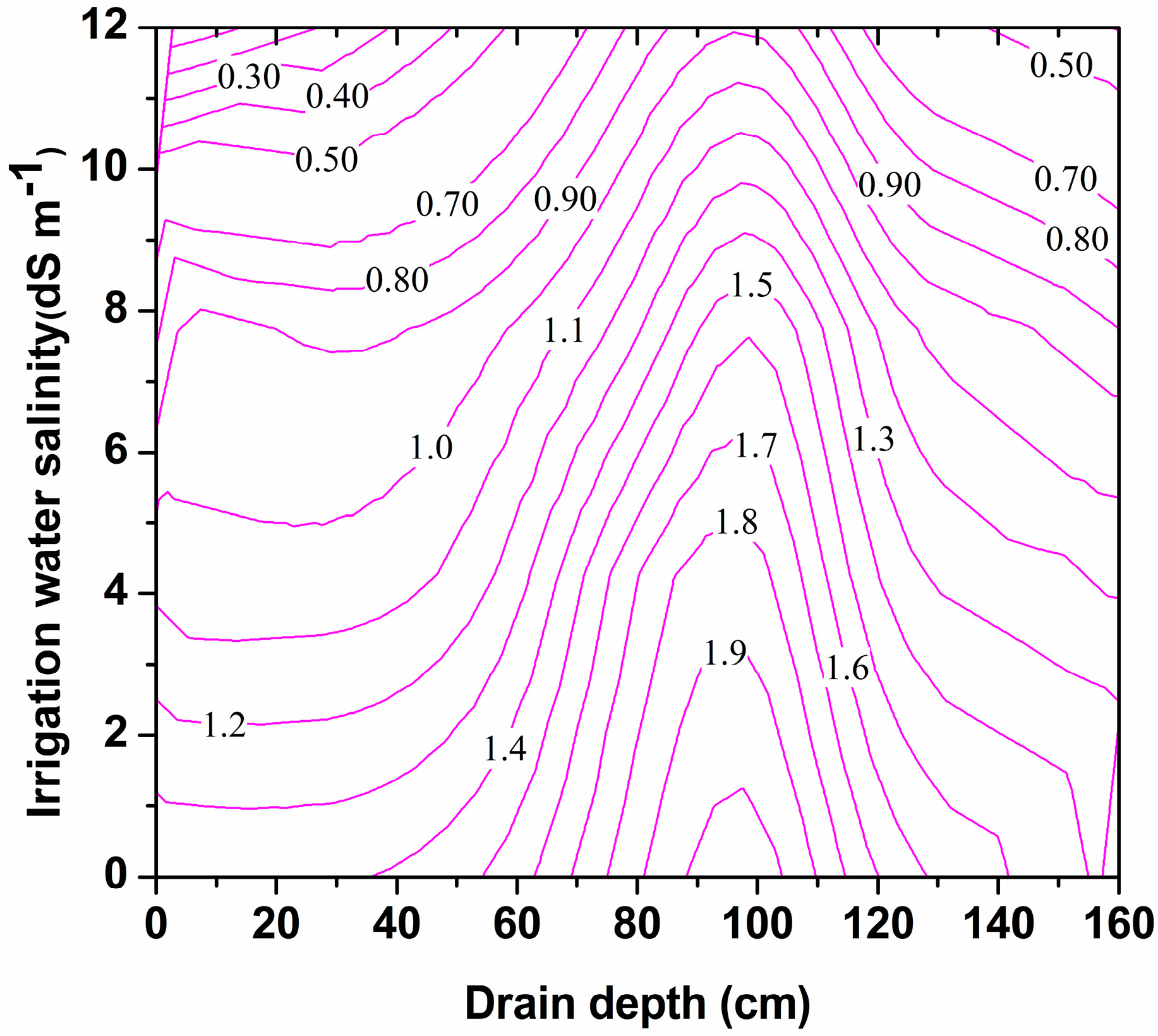
3.3. Optimizing IWS under Subsurface Drainage Condition

As shown in

Table 6. Relationship between relative grain yield and irrigation water salinity (IWS) under different drainage conditions.

Drain Depth (cm)	The Decline Rate 1 (%)	ECiw2(dS m−1)				R2
		Yr = 100%	Yr = 80%	Yr = 50%	Yr = 0%
No subsurface drainage	6.84	0.42	3.35	7.73	15.04	0.96
60	6.04	1.31	4.62	9.59	17.87	0.99
80	6.05	2.89	6.19	11.15	19.41	0.97
100	5.25	4.81	8.61	14.33	22.98	0.95
120	5.93	1.54	4.91	9.97	18.40	0.96
140	6.09	0.70	3.98	8.91	17.12	0.97
160	6.91	0.32	3.70	8.78	17.24	0.96

Note: 1. The decline rate refers to the decline rate of relative yield when irrigation water salinity increased by 1dS m⁻¹; 2. The EC_iw refers to the salinity of irrigation water.

, there were significant linear relationships between relative grain yield and IWS under different drainage conditions, where the determination coefficients R² were greater than 0.95. Under drain depth of 100 and 120 cm, the relative grain yield decreased the least (5.25% and 5.93%, respectively) with increasing IWS. While under drain depth of 160 cm and no subsurface drainage treatments, the relative grain yield decreased the most (6.84% and 6.91%, respectively) with increasing IWS. It should be noted that the threshold values of IWS when summer maize start reducing grain yield production (Y_r = 100%) were different under each drain depth. The highest threshold value of IWS under SDD of 80 and 100 cm were 2.89 and 4.81 dS m⁻¹, respectively. Again, this result confirmed that the effect of salt stress on crop growth was weakened under SDD of 80 and 100 cm. Thus, even under relative higher irrigation water salinity, the growth of corn was not affected obviously. While under SDD of 140, 160, cm and no subsurface drainage condition, the threshold values of IWS were just 0.70, 0.32, and 0.42 dS m⁻¹. The threshold values of IWS when summer maize yield reduction reaches 20% (Y_r = 80%) were also different in each simulation scenario. Under drain depth of 80 and 100 cm, the threshold values of IWS were relatively high, which were 6.19 and 8.61 dS m⁻¹, respectively, while under drain depth of 140, 160 cm and no subsurface drainage condition, the threshold values were much lower than in the other treatments, and they were 3.98, 3.70, and 3.35 dS m⁻¹, respectively. The simulation results above indicated that under drain depth of about 100 cm, the sensitivity of relative grain yield to salt concentration of irrigation water was relatively low. Therefore, based on the results of the scenario simulations and data analysis, it is considered that subsurface drainage condition can provide considerable potential for the sustainable utilization of saline water irrigation.

4. Discussion

4.1. Effects on Soil Salinity

In the two-year field experiment, the soil EC_e within the root zone was significantly reduced during the leaching period: Forty eight days after sowing and 78 days after sowing as shown in Figure 5. The decline range under D0 was much lower than that under other drainage conditions. This phenomenon was caused by the subsurface drainage systems which were installed at different soil depths. Similar studies by Bahceci et al. and Lu et al. suggested that the EC_e within the root zone would reach a relative high level with the increase of IWS [1,53]. The proper depth of subsurface drainage changes with soil properties, soil salinity, and irrigation water salinity [54,55]. Using SALTMOD, Srinivasulu et al. and Ghumman reported that it is not necessary to bury the subsurface pipe to a great depth, when the SDD > 1.4 m, the control of soil water-salt by subsurface drainage would not be meaningful [17]. In our study, simulation results indicated that with SDD around 80~100 cm, EC_e within the root zone could be controlled to a proper level even under relatively high IWS. Therefore, both field experiment and simulation results obtained in this study proved that subsurface drainage condition could control soil water-salt within the root zone with a proper SDD. Moreover, our study confirmed that when subsurface drainage condition is adopted in farmland soil water-salt control, both field experiments and numerical model are essential for evaluating the sustainable utilization of saline water.

4.2. Improved Grain Yield

The grain yield reduction for summer maize was influenced by the root water uptake process, which was affected by water-salt stress within the root zone depth [56]. In the present study, relative grain yield was about 0.80 when IWS was 8.61 dS m⁻¹ and SDD was 100 cm. This result suggested that during the critical growth periods of summer maize, the necessary salt leaching process of the root zone was beneficial for the crops to avoid salt stress. As was reported in previous studies, maize as a moderately salt sensitive crop, when the soil salinity exceeds about 2 dS m⁻¹, the grain yield reduction occurred [57]. Other previous studies also indicated that the reduction rate of grain yield could be retarded with proper irrigation and drainage systems [45,49]. Similar research by Russo indicated that the grain yield reductions were about 8 %and 27%, respectively, at the IWS of 3.6 and 6.7 dS m⁻¹, respectively [58]. However, in their experiment, there was no condition for the salt leaching process during the crop growing seasons. In our study, the reduction rates were much lower, which was about 5.25%–6.91% for every 1 dS m⁻¹ increase in IWS under subsurface drainage condition. Our research confirmed that under proper SDD, the utilization potentiality of saline water irrigation would be remarkably enhanced.

4.3. Ability of the Coupled Model

In our research, the coupled model HYDRUS-EPIC model was used to evaluate the sustainable use of saline water irrigation under subsurface drainage systems. In the field experiment design, the saline water irrigation and subsurface drainage measure were main boundary conditions that affected soil water-salt movement process during the simulation periods. As was reported by previous study, with multiple boundary conditions provided by HYDRUS model, the application ability of HYDRUS model was strengthened [20,21]. With the same model, Tao et al. evaluated the performance of the improved subsurface drainage in Huaibei plain by field experiment and numerical simulation [39]. Ebrahimian and Noory applied HYDRUS-2D model to simulate water flow under subsurface drainage in a paddy field for various drain depths and spacing, surface soil textures, and crack conditions [27]. In crop growth simulation, the EPIC crop growth module used a unified approach to simulate more than 100 types of crops with less input data [43]. When coupled with HYDRUS model, the coupled model had strong advantages in simulating soil hydrological process and crop growth under various condition and crop types [51,52]. In our study, the outputs of current study could be adopted in the design of irrigation schedule under different hydrological year and soil water-salt environment in the future.

5. Conclusions

In the present study, a coupled hydrologic process and crop growth model was evaluated using field experiment data during 2016 and 2017. The coupled model was run to simulate the effects of different IWS and SDD on soil water-salt dynamics, ET, and grain yield of summer maize. The coupled HYDRUS-EPIC model was calibrated and validated adequately by comparing the measured and predicted values from the two growing seasons. A seven × seven scenario simulation was conducted to evaluate the effects of IWS and SDD on relative grain yield and WUE. The results indicated that grain yield reduction could be effectively restrained by the proper arrangement of subsurface drainage system even under high concentration of IWS. Under SDD of 100 cm, the relative yield of summer maize was about 0.82 at IWS of 8 dS m⁻¹ and about 0.53 at IWS of 12 dS m⁻¹. The highest WUE was obtained in the scenario with SDD of 100 cm, and IWS of 0 dS m⁻¹, where WUE reached 2.08 kg m⁻³. A significant linear correlation was found between the relative grain yield of summer maize and the IWS under each drainage condition (R² > 0.95). The optimization results indicated that under drain depth of about 100 cm, the sensitivity of relative grain yield to salt concentration of irrigation water was relatively low in this study. Even when the IWS was as high as 8.61 dS m⁻¹, the yield reduction of summer maize was still less than 20%. In summary, the research indicated that subsurface drainage measures may provide important support for the sustainable utilization of saline water. Moreover, the coupled HYDRUS-EPIC model should be a beneficial tool to evaluate the future sustainability of the saline water irrigation systems.

References

1. Kang, Y.; Chen, M.; Wan, S. Effects of drip irrigation with saline water on waxy maize (Zea mays L. var. ceratina Kulesh) in North China Plain. Agric. Water Manag. 2010, 97, 1303–1309. [Google Scholar] [CrossRef]
2. Amer, K.H. Corn crop response under managing different irrigation and salinity levels. Agric. Water Manag. 2010, 97, 1553–1563. [Google Scholar] [CrossRef]
3. Xue, J.; Ren, L. Conjunctive use of saline and non-saline water in an irrigation district of Yellow River Basin. Irrig. Drain. 2017, 66, 147–162. [Google Scholar] [CrossRef]
4. Ghumman, A.R.; Ghazaw, Y.M.; Niazi, M.F.; Hashmi, H.N. Impact assessment of subsurface drainage on waterlogged and saline lands. Environ. Monit. Assess. 2010, 172, 189–197. [Google Scholar] [CrossRef]
5. He, X.L.; Liu, H.G.; Ye, J.W.; Yang, G.; Li, M.S.; Gong, P.; Aernaguli, A. Comparative investigation on soil salinity leaching under subsurface drainage and ditch drainage in Xinjiang arid region. Int. J. Agric. Biol. Eng. 2016, 9, 109–118. [Google Scholar]
6. Verma, A.K.; Gupta, S.K.; Isaac, R.K. Use of saline water for irrigation in monsoon climate and deep water table regions: Simulation modeling with SWAP. Agric. Water Manag. 2012, 115, 186–193. [Google Scholar] [CrossRef]
7. Rhoades, J.D.; Kandiah, A.; Mashali, A.M. The Use of Saline Waters for Crop Production; FAO Irrigation and Drainage Paper: Rome, Italy, 1992; p. 133. [Google Scholar]
8. Ünlükara, A.; Kurunc, A.; Kesmez, D.G.; Yurtseven, E. Growth and evapotranspiration of okra (Abelmoschus sculentus L.) as influenced by salinity of irrigation water. J. Irrig. Drain. Eng. 2008, 134, 160–166. [Google Scholar]
9. Mathewa, E.K.; Panda, R.K.; Nair, M. Influence of subsurface drainage on crop production and soil quality in a low-lying acid sulphate soil. Agric. Water Manag. 2001, 47, 191–209. [Google Scholar] [CrossRef]
10. Abdullah, D.N.; Ali, S. Influence of subsurface drainage on the productivity of poorly drained paddy fields. Eur. J. Agron. 2014, 56, 1–8. [Google Scholar]
11. Dayyani, S.; Prasher, S.O.; Madani, A.; Madramootoo, C.A. Impact of climate change on the hydrology and nitrogen pollution in a tile-drained agricultural watershed in eastern Canada. Trans. ASABE 2012, 55, 398–401. [Google Scholar] [CrossRef]
12. Sharma, D.P.; Rao, K.V.G.K. Strategy for long term use of saline drainage water for irrigation in semi-arid regions. Agric. Water Manag. 1998, 48, 287–295. [Google Scholar] [CrossRef]
13. Feng, G.X.; Zhang, Z.Y.; Wan, C.Y.; Lu, P.R.; Bakour, A. Effects of saline water irrigation on soil salinity and yield of summer maize (Zea mays L.) in subsurface drainage system. Agric. Water Manag. 2017, 193, 205–213. [Google Scholar] [CrossRef]
14. Sands, G.R.; Song, I.; Busman, L.M.; Hansen, B.J. The effects of subsurface drainage depth and intensity on nitrate loads in the northern corn belt. Trans. ASABE 2008, 51, 937–946. [Google Scholar] [CrossRef]
15. Schultz, B.; Zimmer, D.; Vlotman, W.F. Drainage under increasing and changing requirements. Irrig. Drain. 2007, 56, 3–22. [Google Scholar] [CrossRef]
16. Ayars, J.E.; Meek, D.W. Drainage load–flow relationships in arid irrigated areas. Trans. ASABE 1994, 37, 431–437. [Google Scholar] [CrossRef]
17. Srinivasulu, A.; Sujani Rao, C.; Lakshmi, G.V.; Satyanarayana, T.V.; Boonstra, J. Model studies on salt and water balances at Konanki pilot area Andhra Pradesh. India. Irrig. Drain. Syst. 2004, 18, 11–17. [Google Scholar] [CrossRef]
18. Mehmet, S.K.; Hakan, A. Effects of irrigation water salinity on drainage water salinity, evapotranspiration and other leek (Allium porrum L.) plant parameters. Sci. Hortic. 2016, 201, 211–217. [Google Scholar]
19. Youssef, M.A.; Skaggs, R.W.; Chescheir, G.M.; Gilliam, J.W. Field evaluation of a model for predicting nitrogen losses from drained lands. J. Environ. Qual. 2006, 35, 2026–2042. [Google Scholar] [CrossRef]
20. Karandish, F.; Simunek, J. A field-modeling study for assessing temporal variations of soil-water-crop interactions under water-saving irrigation strategies. Agric. Water Manag. 2016, 178, 291–303. [Google Scholar] [CrossRef]
21. He, Y.; Hu, L.; Wang, H.; Huang, Y.F.; Chen, D.L.; Li, B.G.; Li, Y. Modeling of water and nitrogen utilization of layered soil profiles under a wheat–maize cropping system. Math. Comput. Model. 2013, 58, 596–605. [Google Scholar] [CrossRef]
22. Ghazouani, H.; Autovino, D.; Rallo, G.; Douh, B.; Provenzano, G. Using HYDRUS-2D model to assess the optimal drip lateral depth for eggplant crop in a sandy loam soil of central Tunisia. Ital. J. Agrometeorol. 2016, 21, 47–58. [Google Scholar]
23. Roberts, T.; Lazarovitch, N.; Warrick, A.W.; Thompson, T.L. Modeling salt accumulation with subsurface drip irrigation using HYDRUS-2D. Soil Sci. Soc. Am. J. 2009, 73, 233–240. [Google Scholar] [CrossRef]
24. Chen, L.J.; Feng, Q.; Li, F.R.; Li, C.S. A bidirectional model for simulating soil water flow and salt transport under mulched drip irrigation with saline water. Agric. Water Manag. 2014, 146, 24–33. [Google Scholar] [CrossRef]
25. Rallo, G.; Baiamonte, G.; ManzanoJuárez, J.; Provenzano, G. Improvement of FAO-56 model to estimate transpiration fluxes of drought tolerant crops under soil water deficit: Application for olive groves. J. Irrig. Drain. 2014, 140, A4014001. [Google Scholar] [CrossRef]
26. Tao, Y.; Wang, S.; Xu, D.; Qu, X. Experiment and analysis on flow rate of improved subsurface drainage with ponded water. Agric. Water Manag. 2016, 177, 1–9. [Google Scholar] [CrossRef]
27. Ebrahimian, H.; Noory, H. Modeling paddy field subsurface drainage using HYDRUS-2D. Paddy Water Environ. 2015, 13, 477–485. [Google Scholar] [CrossRef]
28. Filipovic, V.; Mallmann, F.J.K.; Coquet, Y.; Simunek, J. Numerical simulation of water flow in tile and mole drainage systems. Agric. Water Manag. 2014, 146, 105–114. [Google Scholar] [CrossRef]
29. Zhou, J.; Cheng, G.D.; Hu Bill, X.; Wang, G.X. Numerical modeling of wheat irrigation using coupled HYDRUS and WOFOST models. Soil Sci. Soc. Am. J. 2012, 76, 648–662. [Google Scholar] [CrossRef]
30. Xu, X.; Huang, G.H.; Sun, C.; Pereira, L.S.; Ramos, T.B.; Huang, Q.Z.; Hao, Y.Y. Assessing the effects of water table depth on water use, soil salinity and wheat yield: Searching for a target depth for irrigated areas in the upper Yellow River basin. Agric. Water Manag. 2013, 125, 46–60. [Google Scholar] [CrossRef]
31. Wang, J.; Huang, G.H.; Zhan, H.B.; Mohanty, B.P.; Zheng, J.H.; Huang, Q.Z.; Xu, X. Evaluation of soil water dynamics and crop yield under furrow irrigation with a two-dimensional flow and crop growth coupled model. Agric. Water Manag. 2014, 141, 10–22. [Google Scholar] [CrossRef]
32. Wang, X.P.; Huang, G.H.; Yang, J.S.; Huang, Q.Z.; Liu, H.J.; Yu, L.P. An assessment of irrigation practices: Sprinkler irrigation of winter wheat in the North China Plain. Agric. Water Manag. 2015, 159, 197–208. [Google Scholar] [CrossRef]
33. Han, M.; Zhao, C.Y.; Simunek, J.; Feng, G. Evaluating the impact of groundwater on cotton growth and root zone water balance using Hydrus−1D coupled with a crop growth model. Agric. Water Manag. 2015, 160, 64–75. [Google Scholar] [CrossRef]
34. Wang, X.; Liu, G.; Yang, J.; Huang, G.; Yao, R. Evaluating the effects of irrigation water salinity on water movement, crop yield and water use efficiency by means of a coupled hydrologic/crop growth model. Agric. Water Manag. 2017, 185, 13–26. [Google Scholar] [CrossRef]
35. Jiang, J.; Huo, Z.; Feng, S.; Zhang, C. Effect of irrigation amount and water salinity on water consumption and water productivity of spring wheat in Northwest China. Field Crop. Res. 2012, 137, 78–88. [Google Scholar] [CrossRef]
36. Kahown, M.A.; Azam, M. Effect of saline drainage effluent on soil health and crop yield. Agric. Water Manag. 2003, 62, 127–138. [Google Scholar] [CrossRef]
37. Youngs, E.G.; Leeds-Harrison, P.B. Improving efficiency of desalinization with subsurface drainage. J. Irrig. Drain. Eng. ASC 2000, 126, 375–380. [Google Scholar] [CrossRef]
38. Christen, E.W.; Ayars, J.E.; Hornbuckle, J.W. Subsurface drainage design and management in irrigated areas of Australia. Irrig. Sci. 2001, 21, 35–43. [Google Scholar] [CrossRef]
39. Tao, Y.; Wang, S.; Xu, D.; Qu, X.; Yuan, H.W.; Chen, H.R. Field and numerical experiment of an improved subsurface drainage system in Huaibei plain. Agric. Water Manag. 2017, 194, 24–32. [Google Scholar] [CrossRef]
40. Kumar, P.; Sarangi, A.; Singh, D.K.; Parihar, S.S.; Sahoo, R.N. Simulation of saltdynamics in the root zone and yield of wheat crop under irrigated saline regimes using SWAP model. Agric. Water Manag. 2015, 148, 72–83. [Google Scholar] [CrossRef]
41. Van Genuchten, M.T. A Numerical Model for Water and Solute Movement in and Below the Root Zone; Research Report; U.S. Salinity Laboratory: California, CA, USA, 1987. [Google Scholar]
42. Williams, J.R. The EPIC Model. In Computer Models of Watershed Hydrology; Singh, V.P., Ed.; Water Resources Publications: Highlands Ranch, CO, USA, 1995; pp. 909–1000. [Google Scholar]
43. Wöhling, T.; Schmitz, G.H. Physically based coupled model for simulating 1D surface-2D subsurface flow and plant water uptake in irrigation furrow: Model development. J. Irrig. Drain. Eng. 2007, 133, 538–547. [Google Scholar] [CrossRef]
44. Feddes, R.A.; Kowalik, P.J.; Zaradny, H. Simulation of field water use and crop yield. Field Crops Res. 1980, 3, 95–96. [Google Scholar]
45. Monsi, M.; Saeki, T. Uber den Lictfaktor in den Pflanzen-gesellschaften und seine Bedeutung fur die Stoffproduktion. Jpn. J. Bot. 1953, 14, 22–52. [Google Scholar]
46. Monteith, J.L. Principles of Environmental Physics; Edward Arnold: London, UK, 1973. [Google Scholar]
47. Uchijima, Z.; Udagawa, T.; Horie, T.; Kobayashi, K. The penetration of direct solar radiation into corn canopy and the intensity of direct radiation on the foliage surface. J. Agron. Meteorol. Tokyo 1968, 3, 141–151. [Google Scholar] [CrossRef]
48. Wesseling, J.G. Meerjarige Simulaties van Grondwateromttrekking voor Verschillende Bodemprofielen, Grondwatertrappen en Gewassen Met Het Model SWATRE; Report 152; DLO-Staring: Wageningen, The Netherlands, 1991. [Google Scholar]
49. Siyal, A.A.; van Genuchten, M.T.; Skaggs, T.H. Solute transport in a loamy soil under subsurface porous clay pipe irrigation. Agric. Water Manag. 2013, 121, 73–80. [Google Scholar] [CrossRef]
50. Ren, D.Y.; Xu, X.; Hao, Y.Y.; Huang, G.H. Modelling and assessing field irrigation water use in a canal system of Hetao, upper Yellow River basin: Application to maize, sunflower and watermelon. J. Hydrol. 2016, 532, 122–139. [Google Scholar] [CrossRef]
51. Wang, X.C.; Li, J. Evaluation of crop yield and soil water estimated using the EPIC model for the Loess Plateau of China. Math. Comput. Model. 2010, 51, 1390–1397. [Google Scholar] [CrossRef]
52. Wang, X.P.; Huang, G.H. Evaluation on the irrigation and fertilization management practices under the application of treated sewage water in Beijing, China. Agric. Water Manag. 2008, 95, 1011–1027. [Google Scholar] [CrossRef]
53. Bahceci, I.; Cakir, R.; Nacar, A.S.; Bahceci, P. Estimating the effect of controlled drainage on soil salinity and irrigation efficiency in the Harran Plain using SaltMod. Turk. J. Agric. For. 2008, 37, 101–109. [Google Scholar]
54. Lu, P.R.; Zhang, Z.Y.; Feng, G.X.; Huang, M.Y.; Shi, X.F. Experimental study on the potential use of bundled crop straws as subsurface drainage material in the newly reclaimed coastal land in Eastern China. Water 2018, 10, 31. [Google Scholar] [CrossRef] [Green Version]
55. Joseph, S.; Husson, O.; Graber, E.; Van Zwieten, L.; Taherymoosavi, S.; Thomas, T.; Nielsen, S.; Ye, J.; Pan, G.; Chia, C. The electrochemical properties of biochars and how they affect soil redox properties and processes. Agronomy 2015, 5, 322–340. [Google Scholar] [CrossRef] [Green Version]
56. Zheng, C.; Jiang, D.; Liu, F.; Dai, T.; Jing, Q.; Cao, W. Effects of salt and waterlogging stresses and their combination on leaf photosynthesis, chloroplast ATP synthesis, and antioxidant capacity in wheat. Plant Sci. 2009, 176, 575–582. [Google Scholar] [CrossRef] [PubMed]
57. Mass, E.V.; Grattan, S.R. Crop Yields as Affected by Salinity. In Agricultural Drainage; Skaggs, R.W., van Schilfgaarde, J., Eds.; ASA: Madison, WI, USA; CSSA: Fitchburg, MA, USA; SSSA: Madison, WI, USA, 1999; pp. 55–108. [Google Scholar]
58. Russo, D.; Bakker, D. Crop–water production functions for sweet corn and cotton irrigated with saline waters. Soil Sci. Soc. Am. J. 1987, 51, 1554–1562. [Google Scholar] [CrossRef]
Figure 1. (a) The layout of the lysimeter; (b) the profile map of the lysimeter.
Sustainability 11 06431 g001
Figure 2. Daily values of temperature, and irrigation events during 2016 and 2017 growing seasons.
Sustainability 11 06431 g002
Figure 3. The observed and predicted soil water contents at sowing time (a) and harvest time (b) during calibration (2016).
Sustainability 11 06431 g003
Figure 4. The observed and predicted soil water contents during validation (2017).
Sustainability 11 06431 g004
Figure 5. The observed and predicted ECe within the root zone depth during calibration (2016).
Sustainability 11 06431 g005
Figure 6. The observed and predicted ECe within the root zone depth during validation (2017).
Sustainability 11 06431 g006
Figure 7. Contour map of the relative grain yield in each simulation scenario.
Sustainability 11 06431 g007
Figure 8. Contour map of the water use efficiency (WUE) in each simulation scenario.
Sustainability 11 06431 g008