Holiday Travel Behaviour and Correlated CO2 Emissions—Modelling Trend and Future Scenarios for Austrian Tourists

Kapeller, Marie Lisa; Füllsack, Manfred; Jäger, Georg

doi:10.3390/su11226418

Open AccessArticle

Holiday Travel Behaviour and Correlated CO₂ Emissions—Modelling Trend and Future Scenarios for Austrian Tourists

by

Marie Lisa Kapeller

^*

,

Manfred Füllsack

and

Georg Jäger

^*

Institute of Systems Sciences, Innovation and Sustainability Research, University of Graz, 8010 Graz, Austria

^*

Authors to whom correspondence should be addressed.

Sustainability 2019, 11(22), 6418; https://doi.org/10.3390/su11226418

Submission received: 7 October 2019 / Revised: 11 November 2019 / Accepted: 12 November 2019 / Published: 15 November 2019

(This article belongs to the Section Sustainable Transportation)

Download

Browse Figures

Versions Notes

Abstract

:

The footprint of tourism through travel is contributing significantly to the accumulation of human-made CO₂. Due to different options in transportation, resulting emissions depend strongly on the choices of individuals on how to travel. In Austria, land travel is the main mode of transportation, though air travel has shown a significant increase during the last decades. We present a model to estimate past and future emission trends of land and air travel for domestic (inbound) and international (outbound) travel destinations. For this, we use a combination of two software models, a social-economic individual-based model to simulate the decision processes of holiday travel and an emission calculation model to estimate single travel-based CO₂ emissions. Our model is supported by data (reference year 2016) on tourism demand, holiday destinations, household wealth and emissions of different transportation modes. Our model evaluation successfully reproduced historical data of travel demand in the period 2003–2019 and explores several future trends of (a) business-as-usual, (b) green transition and (c) aviation preference increase. We calculated a current CO₂ footprint of 5.8 million tonnes in 2019, which could increase to 7.3 million tonnes by 2030 if the current trend continues. A necessary decrease of transportation emissions is only possible when reducing air travel. In case of a green transition towards more land travel, total emissions could be kept constant compared to current emission levels. However, an overall reduction of holiday travel related CO₂ below 3.5 million tonnes has not been observed even under the best circumstances due to projected increases in the total population and increases in wealth.

Keywords:

tourism; Austria; travel; emissions; agent-based model; greenhouse gases; transportation

1. Introduction

The transportation sector is responsible for a major fraction of global CO₂ emissions. In the European Union, more than 22% of all greenhouse gas (GHG) emissions are caused by transport [1]. However, this large share does not necessarily mean that there is an equally large potential to reduce emissions. One has to take a closer look at the individual segments to identify possibilities to reduce CO₂ emissions without major drawbacks for society or individuals. Transporting essential goods or commuting to work are necessities, for which it is difficult to find suitable substitutes that produce fewer emissions.

For other segments of transportation, however, there is ample opportunity to reduce emissions. One of these segments, on which this study will focus, are emissions caused by tourism-related transport. First of all, going on holiday is a luxury in the sense that it is not vital, in contrast to other causes of transportation-related emissions. Secondly, even if we want to preserve this luxury, there are many ways to save emissions by choosing the destination and the mode that is used to reach that destination carefully. Improvements in that sector would have significant effects, especially considering that travel and tourism is one of the world’s largest economic sectors. Holidays of middle class households alone contribute 10.4% to the global GDP [2]. Within the tourism segment, the main contribution of GHG emissions comes from aviation (40% of tourism’s overall carbon footprint) followed by car transportation (32%).

Unfortunately, this huge potential for reducing emissions is currently not exploited. On the contrary, today’s trend shows a drastic increase in emissions. This has various reasons—first of all, the tourism sector itself is growing rapidly, even faster than international trade [2]. Secondly, aviation as a method of transportation becomes more and more popular. According to the European Aviation Environmental Report 2019, the number of flights increased by 60% between 2005 and 2017. Additionally, the average travelled distance for holiday trips increases continuously [3]. One of the main reasons for this development is the availability of low-cost air fares, which makes destinations accessible that were previously out of reach because of financial or time constraints [4]. Based on a business-as-usual (BAU) growth scenario, IATA predicts that the number of air passengers will nearly double between 2017 and 2037 in its 20 Year Passenger Forecast [5].

If we want to change that trend and find ways to transition towards sustainable tourism, the first step is to gain a deeper understanding of tourism-related transport and resulting emissions. One way of gaining such an understanding would be the evaluation of various scenarios, to see the effects that certain policies or behavioural changes have on GHG emissions. However, such scenarios are difficult to evaluate. Since the choice of whether to go on a holiday or or not, the choice of a destination and the choice of a method of transport largely depend on human decision making and behaviour, simple regressions or extrapolations are insufficient to produce meaningful results. This is why we utilise an agent-based computer model to tackle this challenge. In order to keep the model simple and clear, we limit the scope to a single country. Here we choose Austria, but the presented model would also work for arbitrary countries.

In our model, agents have individual preferences and financial means based on empirical data (see Section 2). They do not act in isolation but are embedded in a social network. During a simulation run they all perform a realistic decision process, which leads to travel destinations and modes that can in the end be translated into GHG emissions (for details on the simulation process, see Section 4). That way we can not only reproduce the status quo for model evaluation, but also explore many possible future scenarios. This analysis then serves as a starting point for further studies.

2. Empirical Background

In order to model tourism travel behaviour of Austrian residents, we use three different data sets on relevant information regarding

(a): tourism holiday demand and trends from 2003–2018,
(b): holiday travel destinations, and
(c): perceived household net wealth distribution.

Parts of this information serve as guidance for the model settings and other parts are used to evaluate the model output.

2.1. Tourism Demand Data of Austria

Statistical survey data on the national travel behaviour of the Austrian population are provided by Statistics Austria [6,7,8]. Our evaluation focuses in particular on the year 2016, as a more detailed data set is available here. Table 1 provides an overview of the statistics. To illustrate the importance of holiday travel in contrast to business travel, the table shows the total travel volume (left), holiday travel (centre) and business travel (right). With only 16% of all travels being business trips, the major drivers to travel are personal.

In 2016, 5.66 out of 7.37 million potential Austrian tourists (citizens above the age of 15) engaged in at least one holiday travel, which corresponds to a total travel intensity of 76.8%. The overall number of holiday trips was 19.7 million. The average number of trips per person is

3.5

which is below the European mean of 4 trips per person. With regard to travel destinations, domestic and outbound tourist destinations are roughly 51.1% and 48.9% respectively.

2.2. Holiday Transportation Modes

The statistical data of the year 2016, given in Table 2, show that Austrian residents prefer land travel (83.1%) over air travel (16.9%). Domestic travel is almost exclusively land travel, resulting in a share of 34.3% of air travel for international destinations. The most common means of transport for land travel is by car, other means of transport such as train and bus have a similar share in both domestic and international travel.

2.3. Holiday Destination Data of Austrian Tourists

Records on holiday travel destinations are provided in the standard documentation and meta-information, Travel habits of the Austrian population 2016 [7]. As shown in Table 3 about half of holidays are domestic, the destination of the other half is distributed over various countries with different shares respectively. Austrian’s top destinations in 2016 are Italy, Germany and Croatia, followed by Spain, Greece and Hungary. The 17 top destinations make up 82.4% of all travels. Minor destinations account for 17.6% of all holiday travels. For some regions the statistical record subsumes several countries without further specification, for example, other European Countries, Algerian/Morocco. The major part of outbound travel remains within Europe (92.6%) while the shares of America, Asia and Africa are equal to or below 3%.

2.4. Household Wealth Data

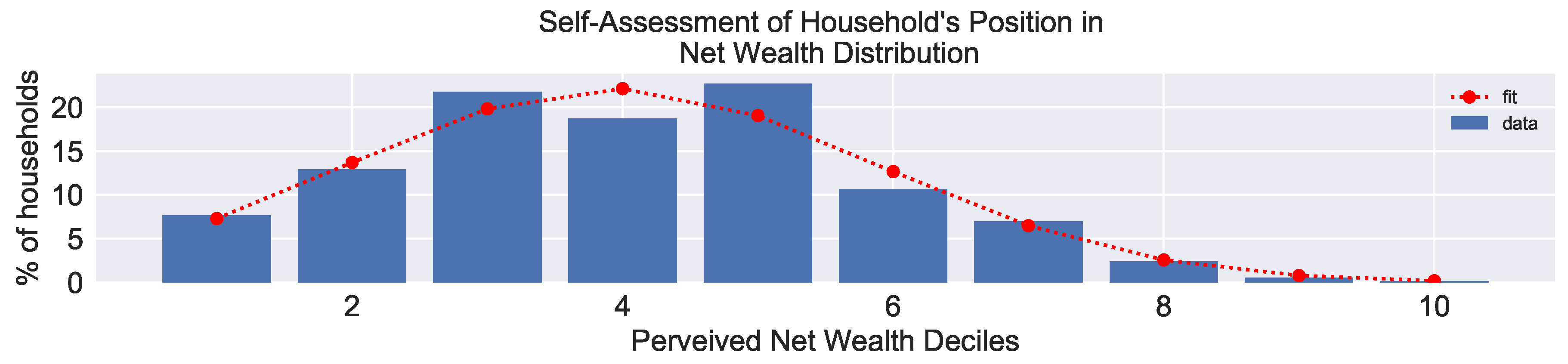
Financial aspects of holiday travels are difficult to capture, since no suitable statistical information on spending habits are available. Thus, we choose to include monetary aspects by perceived net wealth distributions, which reflect the relative expenses a citizen would likely think to be affordable. We believe that holiday decisions are less influenced by what individuals can afford and much more by what they think they can afford. The Eurosystem Household Finance and Consumption Survey 2017 [9] provides data on self-assessment of household’s position in net wealth distribution of Austrian citizens in ten deciles. In Figure 1, we calculated the mean perceived net wealth deciles of the available years 2014 and 2017. To approximate the data via Gaussian distribution (red line), we use a best-fit algorithm resulting in the mean

μ = 3.924

and standard deviation

σ = 1.962

. Note, that the more wealth a household has, the lower the probability of a correct self-assessment and that households at the lower end of the distribution overestimate their wealth decile.

3. Emissions: Land and Air Travel

According to available empirical data, we distinguish primary air and land travel and secondary car and other transportation modes for land travel. Land travel comprise a main share of car travel (

65 %

) and a smaller share of combined bus and rail travel (

18 %

). To calculate emissions of holiday travel we use different transportation modes, for example, car, bus, train and air travel.

Emissions are based on estimated distances from the origin location (Austria) to the holiday destination (domestic or international). Since land travel and air travel utilise different routes, we use the shortest road connection for the former and the bee-line for the latter. We consider direct flight routes and neglect detours. Details on emission data acquisition are given in ‘Material and Methods’ Appendix A.1.1 and Appendix A.4.

Table 4 gives details on holiday land travel to Austrian federal states. The mean distance and correlated CO₂ emissions are shown for car, train and bus travel. The most frequently visited federal states are Styria, Salzburg and Carinthia.

Table 5 shows the collected data of land and air distances and correlated CO₂ emissions top and minor outbound destinations (compare with Table 3). Since land travel is not possible or feasible for all destinations, only air travel is calculated for all countries.

4. Model

The developed model is a combination of two sub-—a decision-making model and an emission calculation model. Both sub-models are based on discrete time steps of one year. First, an agent-based model (ABM) serves to capture the decision process of holiday travel. In each year, agents face multiple holiday decisions. For each decision, they need to determine whether they want to go on a holiday or not, they need to find a suitable travel partner and have the choice between land and air travel. The model calculates the amount of tourists engaging in at least one holiday travel per year, the number of individuals who did not engage in a holiday, the amount of trips and the amount of land and air trips. The model is capable to capture the status quo and the associated trend over the time-span of 2003–2030. Future scenario modulation of 2020–2030 is very flexible and in order to showcase its capabilities we present the following scenarios:

(A): Green Transition and
(B): Aviation Preferences

Details about the ABM and the decision-tree are shown in ‘Material and Methods’ Appendix A.2.

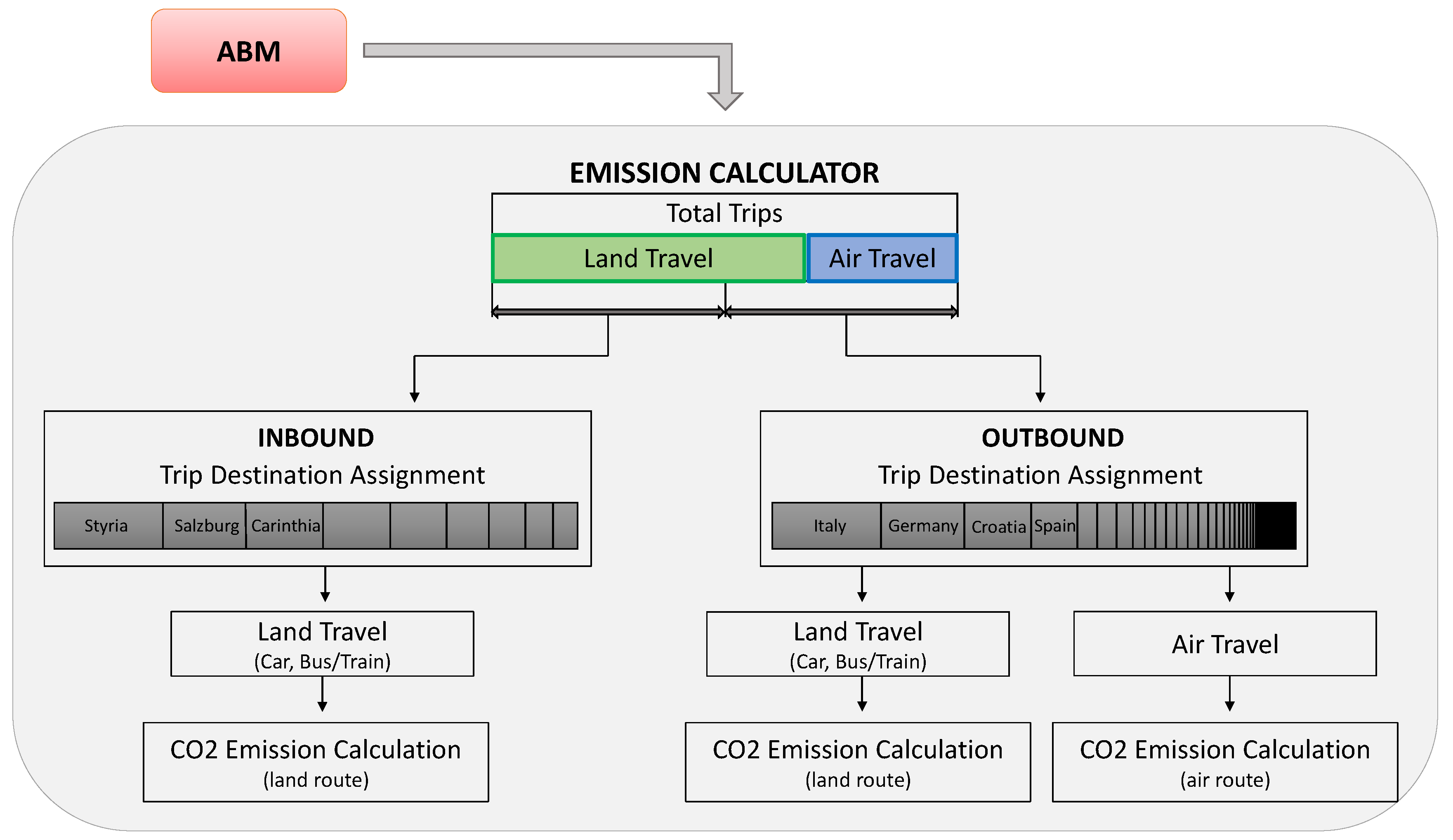
The second sub-model calculates CO₂ emissions based on information from the ABM output of the amount of trips, the amount of land travel and the number of air travels. The model distinguishes inbound and outbound trips. Inbound trips are considered to be land travel exclusively, outbound trips have a flexible ratio of land and air travel, depending on the ABM generated travel data. The model assigns each trip a holiday destination and transportation mode to reach this destination. The CO₂ emissions can be calculated for inbound land travel, outbound land travel, outbound air travel and total trips per year. The model is capable to capture trends and scenarios calculated by the decision-based ABM. Details about the emission calculation model are given in ‘Material and Methods’ Appendix A.3.

The model setup is designed to engage in the following questions:

What is the yearly tourism travel demand of Austrian residents (above 15 years old) in the period 2003 to 2030? What are the observed trends and future projections from an empirical and modelled standpoint?
What are yearly CO₂ emissions stemming from holiday travel for both, aviation and land transportation including cars, train and bus? How much did the travel footprint increase in the time-span 2003–2018 and what are future prospects of increased travel demand?
Engaging in different future scenarios, how do financial or social aspects induce shifts in holiday travel demand?
What could be a possible effect of increasing the cheap flight contingent on the overall holiday travel footprint?
What could be a possible effect of shifts in preferences between land and air travel?
What is the estimated contribution of Austrian holiday air travel to the global air travel emissions?

4.1. Scenarios

To expand the discussion on possible future development of holiday travel of Austrian citizens, we present three scenarios which we investigate and compare to the results of the extrapolation of the status quo. These scenarios are abstract implementations and serve as an indicator to estimate possible increases or decreases in CO₂ emissions for different travel modes.

4.1.1. Green Transition

As tourism travel is an activity that shows increasing emissions over the past decades, we consider a scenario that includes favourable conditions potentially leading to a reduction in greenhouse gas emissions. For this purpose, we regard a combined policies approach in aviation ticket pricing, public transportation and destination preferences. Other possibilities of influencing human decision making include ecological education, for which national parks can play an important role [10], especially for Austria.

In regard to aviation, one widely investigated policy that can be used to decrease carbon emissions is to tax products or services that lead to GHG emissions. This can be done in various ways. One could introduce a carbon tax [11,12,13], tax kerosene [14], include aviation in the European emissions trading scheme [15] or introduce a ticket tax [16].

Independent of how a tax on aviation is actually implemented, it would lead to a financial incentive to decide against flying long distances. Within our model, this would mean that destinations that are far away would get more expensive and thus become less attractive, relating to a preference shift of international destinations.

In the 1980s, a large share of bus and train traffic was shifted to air traffic while the share of car travel remained nearly the same. This reduced the share of public transport to an average of 18%. This change in preferences was followed by a sharp increase in associated travel emissions.

We implement a ‘green transition’ scenario that involves an annual increase in the price of airline tickets, an increase of public transportation share from 18% to 25% and a small preference shift of travel destinations from minor destinations, such as Oceania and South Korea, depending on the actual amount of total air travel.

4.1.2. Aviation Preferences

In contrast to improving emissions through appropriate policies, it is also conceivable that there may be additional trends that exceed the actual increase in business-as-usual emissions. An important factor here is the self-regulation of air prices, which for years indicates a tendency to offer ever cheaper flights and a larger contingent of low-cost flights. In recent years low-cost airlines became more and more relevant for aviation, especially for tourists [17,18,19]. Likewise, a further decline in the use of public transport would be possible by increasing the share of flights. Thirdly, over-cheap flight options could also shift preferences to long-haul flights.

We implement an ‘aviation preference’ scenario that involves an annual decrease in the price of airline tickets, an decrease of public transportation share from 18% to 11% and a small preference shift of travel destinations towards minor destinations in correlation to the actual amount of total air travel.

4.2. Simulations

The ABM output is a yearly amount of trips and corresponding shares of land and air travel and the calculated CO₂ emissions for inbound travel (land) and outbound travel (land, air). For the status-quo investigation, we simulate the period 2003–2019, for current trend and other future scenario investigation we simulate 2020–2030. In accordance to the available empirical data, the reference year is 2016, for which we use the following initialisation and settings:

Financial Aspects: the mean wealth distribution is according to the Gaussian curve of the perceived net wealth in Figure 1.
Destination Assignment: Outbound destinations are statistically chosen according to the empiric data on travel destinations of Table 3. Similarly, inbound travel to different federal states are statistically distributed to the respective shares given in Table 4.
Calculation of emissions are based on Table 4 and Table 5.

The resulting amount of tourists and travels are not data-forced but an emergent phenomena of the agent’s decision process. To account for trends in tourist and travel amounts, we use the following adaptations from the reference year:

Financial Aspects: A yearly mean wealth shift estimates relative changes in spending behaviour. This shift is negative for the year before 2016 and positive for the year after 2016.
Destination Assignment: Inbound travel to different federal states remain unchanged. Outbound destinations shares remain unchanged only for the status-quo investigation and most scenarios except of the kerosene tax scenario. For the latter, we reduce the number of minor destinations slightly. For all trend simulations, the land–air ratio of outbound destinations undergoes a small yearly shift which is related to increases or decreases of the amount of air travel contingent in respect of the total amount of trips.

Further information on variables, trend fitting and general model settings are given in ‘Material and Methods’ Appendix A in detail.

5. Results

The business-as-usual (BAU) growth scenario represents the primary investigation of the model capabilities of the ABM. We show a comparison of model data with empirical trends of Austrian tourism in the period 2003–2030. This trend analysis is followed by the emission calculation of the respective period for land and air travel.

This primary investigation on the model capabilities is followed by three scenarios. The first scenario refers to a price decline for air travel due to an increase in low-cost ticket contingent. Second scenario pictures a continuous increase air ticket prices for example due to kerosene tax. The third scenario is a change in travel habits. Similar to the 1980s, when there was a change in the preference for rail and train travel for air travel, which led to a rapid increase in the proportion of air travel within a few years, we use the model to look at a situation in which car travel is becoming less popular and is being replaced by air travel.

5.1. Reference Year 2016

With the reference year 2016 for the empirical information, we compare the respective model data in Table 6. To consider sampling error, we include a small 5% statistical deviation for all data. The model statistics are shown for average and standard deviation of 100 simulations. The model evaluation shows an excellent overlap for all travel related data. The modelled share of tourists and non-tourists shows a good reflection of empirical data with a discrepancy below 10%.

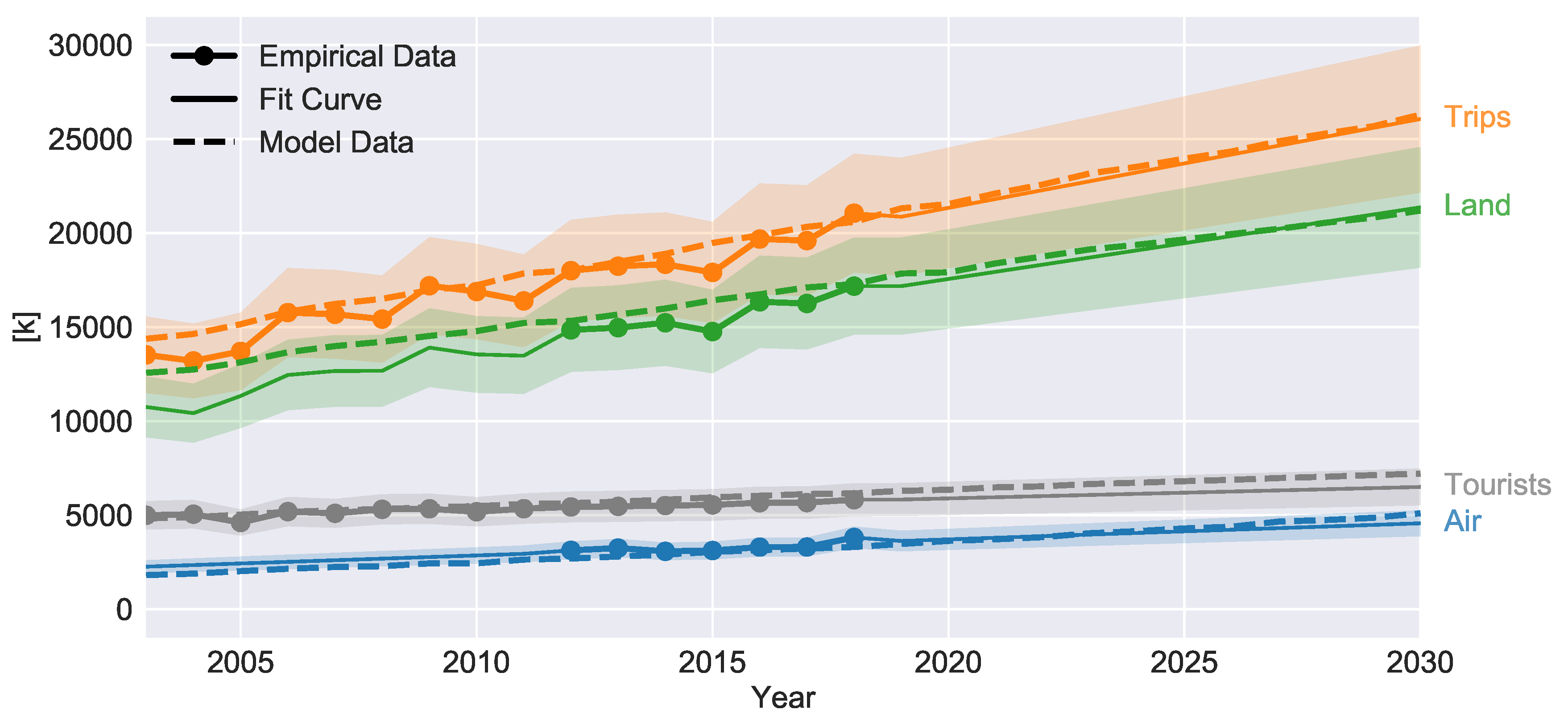
5.2. Trend Analysis: Business-As-Usual (BAU)

The trend analysis of holiday travel demand is shown in Figure 2. Survey data of Statistics Austria marked by dots serves as a baseline for the trend extrapolation shown via solid lines. Modelled data (dashed lines) show similar trends in terms of increases in tourism over the whole time range of almost 30 years. However, a small overestimation of land travel and underestimation of air travel is visible for 2003–2005. We conclude that most part of the development in tourism for the BAU scenario can be reproduced by a simple population increase and continuous growth in population wealth.

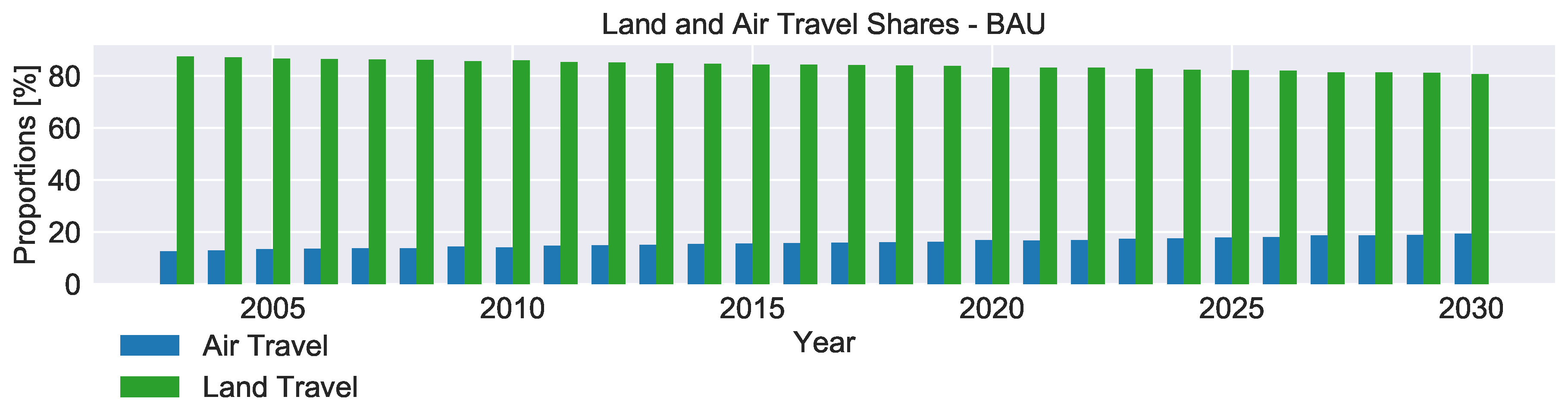
Figure 3 shows the proportion of land and air travel from 2003–2030 for domestic and international travel. Land travel shows the largest share even if there is a trend towards air travel. This trend increases the share of flights from 12.6 % (2003) to 19.4% (2030).

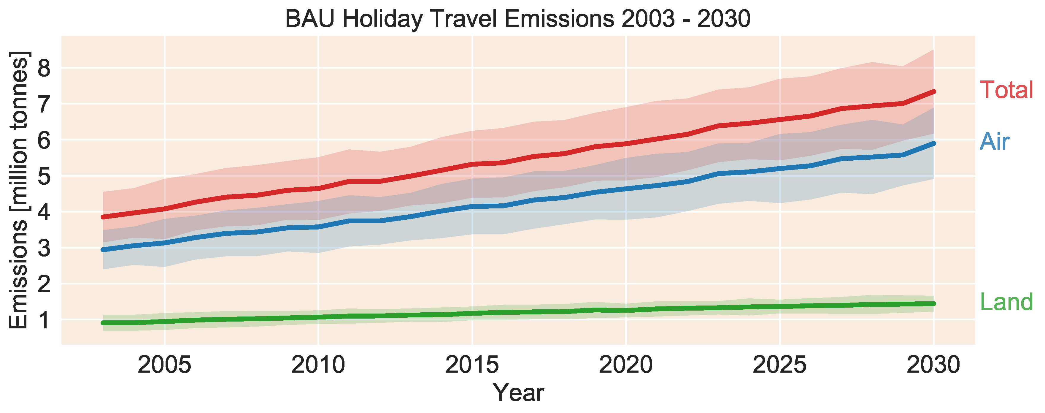
Based on travel demand, we calculate the emissions of Austrian holiday travel behaviour. The results for the BAU scenario are shown in Figure 4. Current emissions from holiday travel are 5.8 million tonnes (2019) and emissions are expected to rise to 7.28 million tonnes by 2030 if the current trend continues. In 2003–2019, land travel emissions increased about 0.35 million tonnes while air travel increased about four times higher by 1.6 million tonnes. The air travel share accounts for almost 80% (2019) of all travel emissions and this share is continuously increasing.

5.3. Scenario Analysis: Travel Behaviour Trends

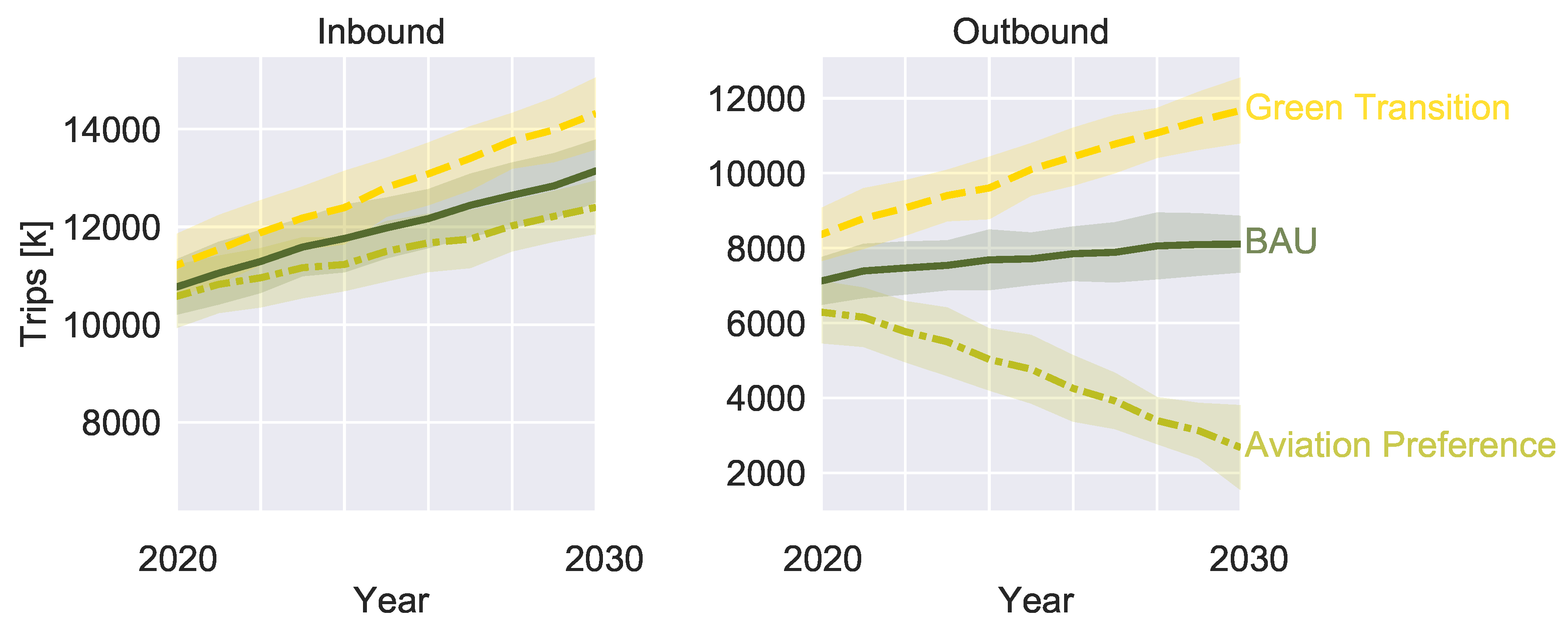
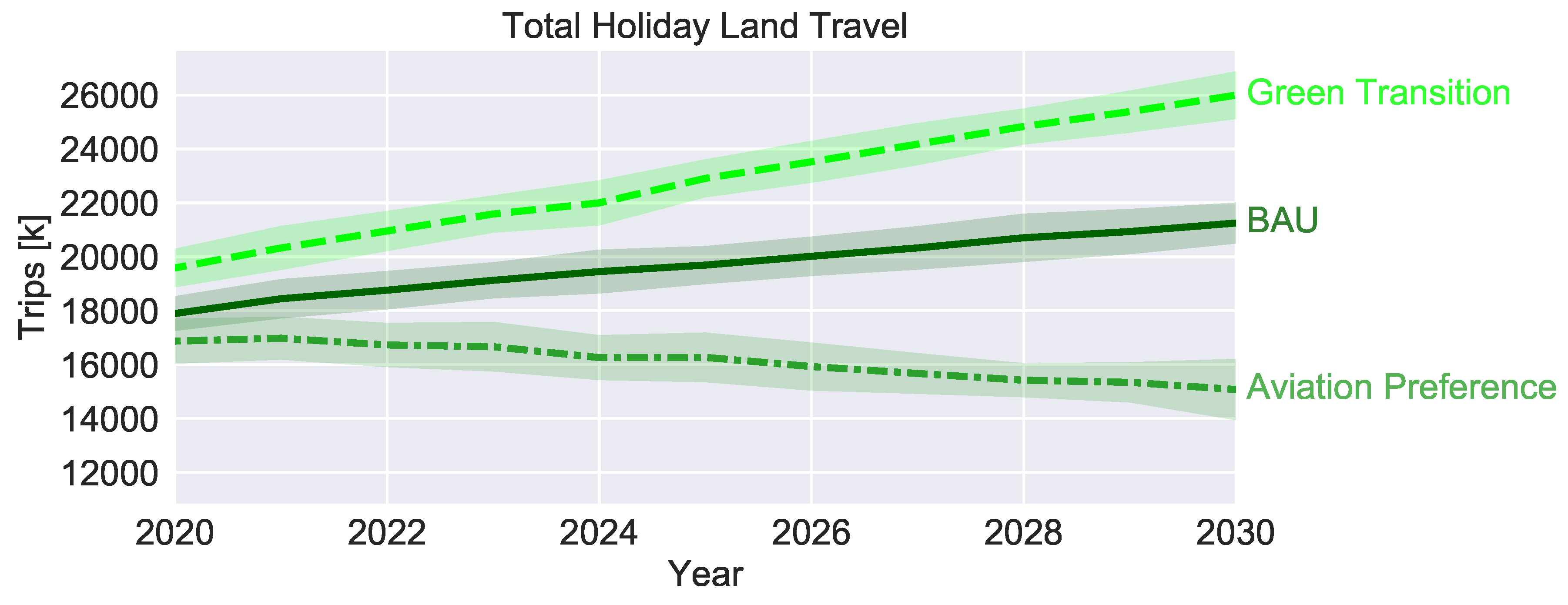
Regarding different possible trends beyond business-as-usual, we show holiday trends for alternative future developments via two additional scenarios. Figure 5, Figure 6, Figure 7 and Figure 8 show the results for the BAU scenario (solid line), the ‘Green Transition’ scenario (dashed line), and ‘Aviation Preference’ scenario (dashed-dotted line). For domestic travel (Figure 5), land travel increases for all scenarios with the highest increase for ‘Green Transition.’ For international travel by car, bus and train, a strong increase in land travel occurs in scenario ‘Green Transition,’ while the scenario ‘Aviation Preference’ leads to a strong decrease in land travel. The total number of trips in the scenario ‘Green Transition’ shows an overall stronger increase compared to the other two cases due to a stronger increase in land travel.

Trends in Land—Air Proportions

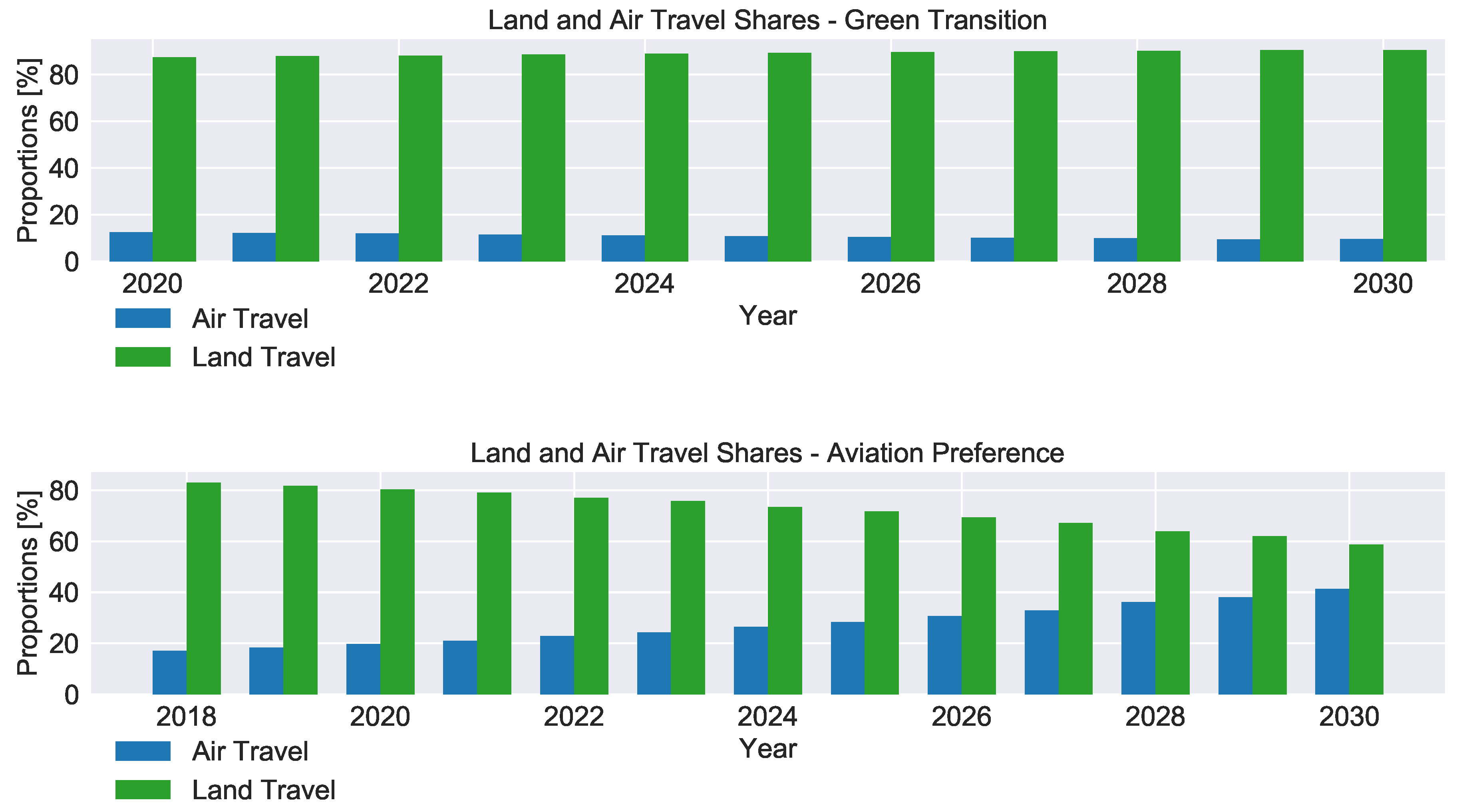
Shifts in the proportions of land and air travel are shown in Figure 9. In the scenario ‘Green Transition’ (top) a decrease of air travel to 9.53% (2030) is observed while in the scenario ‘Aviation Preference’ (bottom) air travel is skyrocketing towards 41.3%.

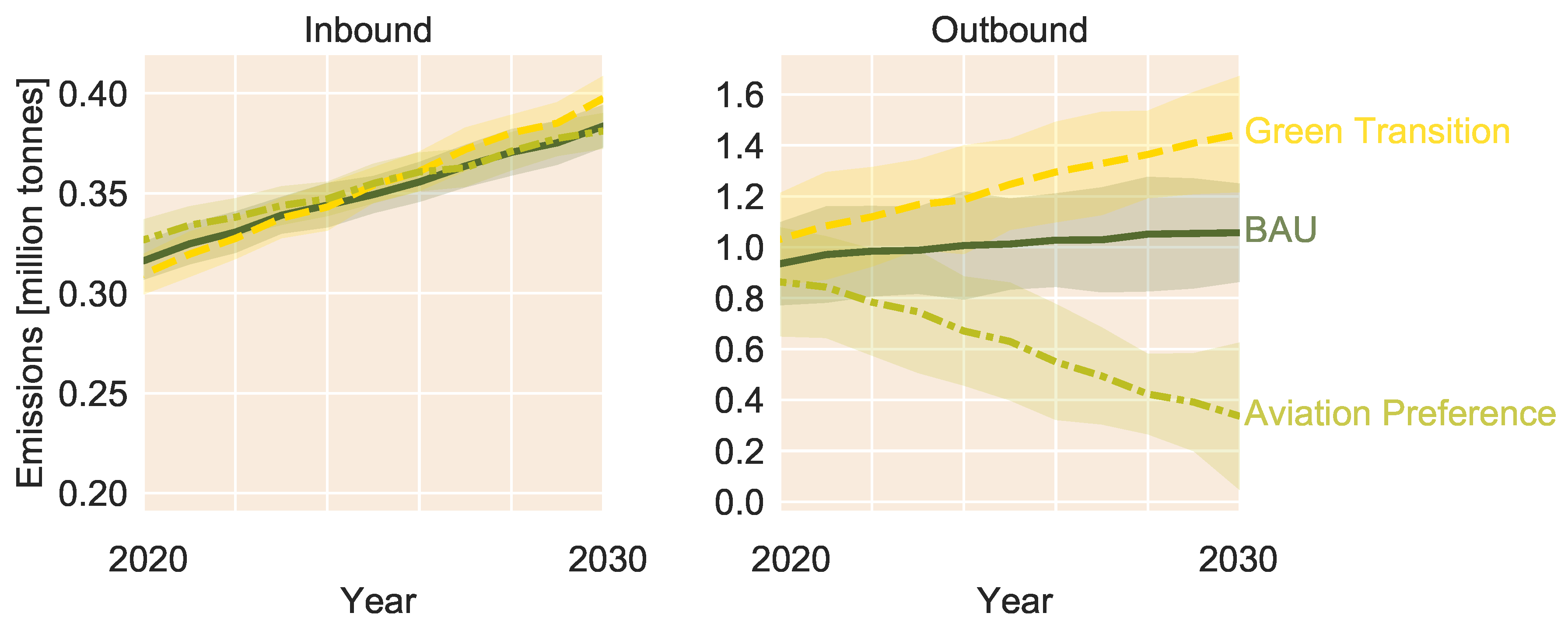
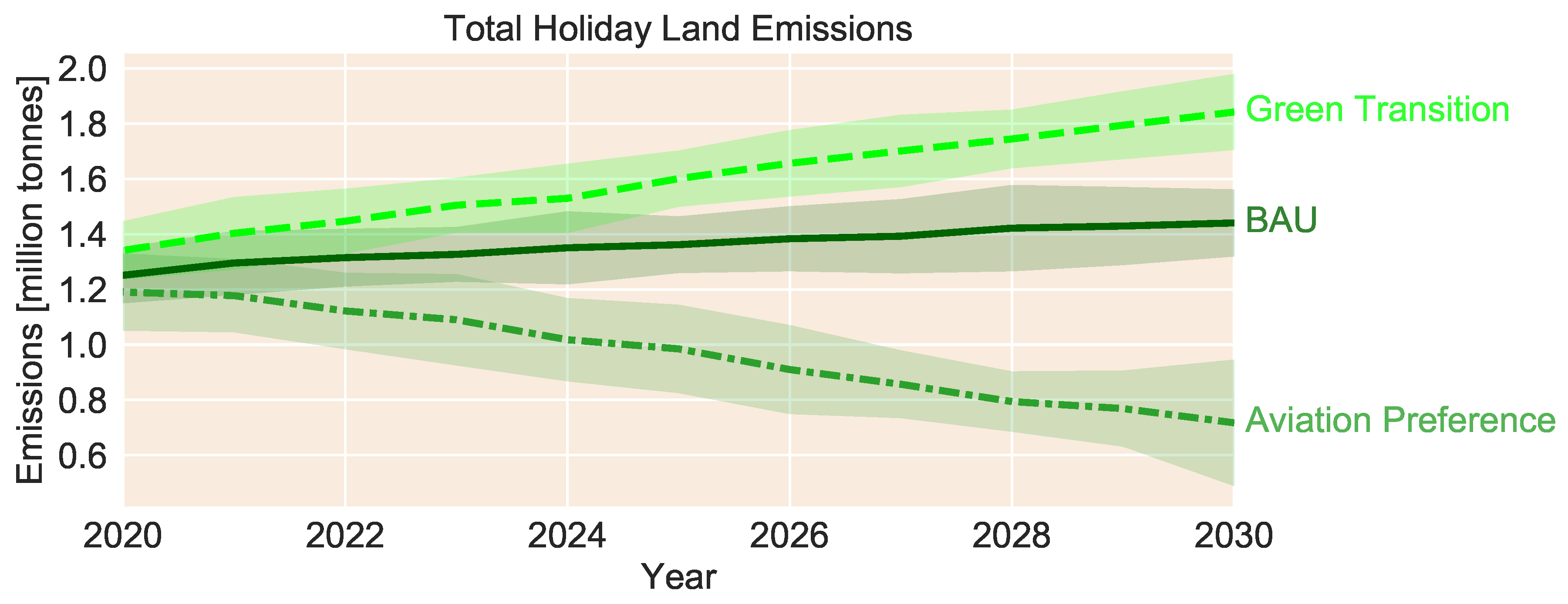
5.4. Scenario Analysis: Emission Trends

We present emissions calculations for all three scenarios, namely BAU, ‘Green Transition’ and ‘Aviation Preference.’ Emissions of domestic holiday land travel (Figure 10 left) shows a strong overlap in all scenarios while international land travel (Figure 10 right) show a string increase for the ‘Green Transition’ and a strong decline for the ‘Aviation Preference.’ Combined domestic and international land travel (Figure 11) reveals a similar pattern to that visible for international travel due to an overall higher amount of CO₂ emissions.

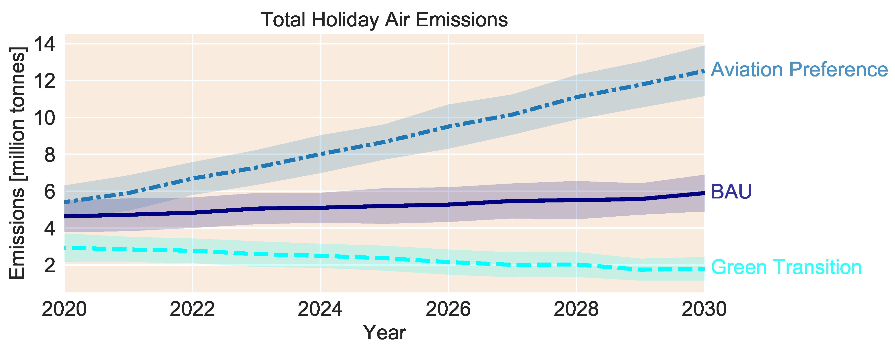
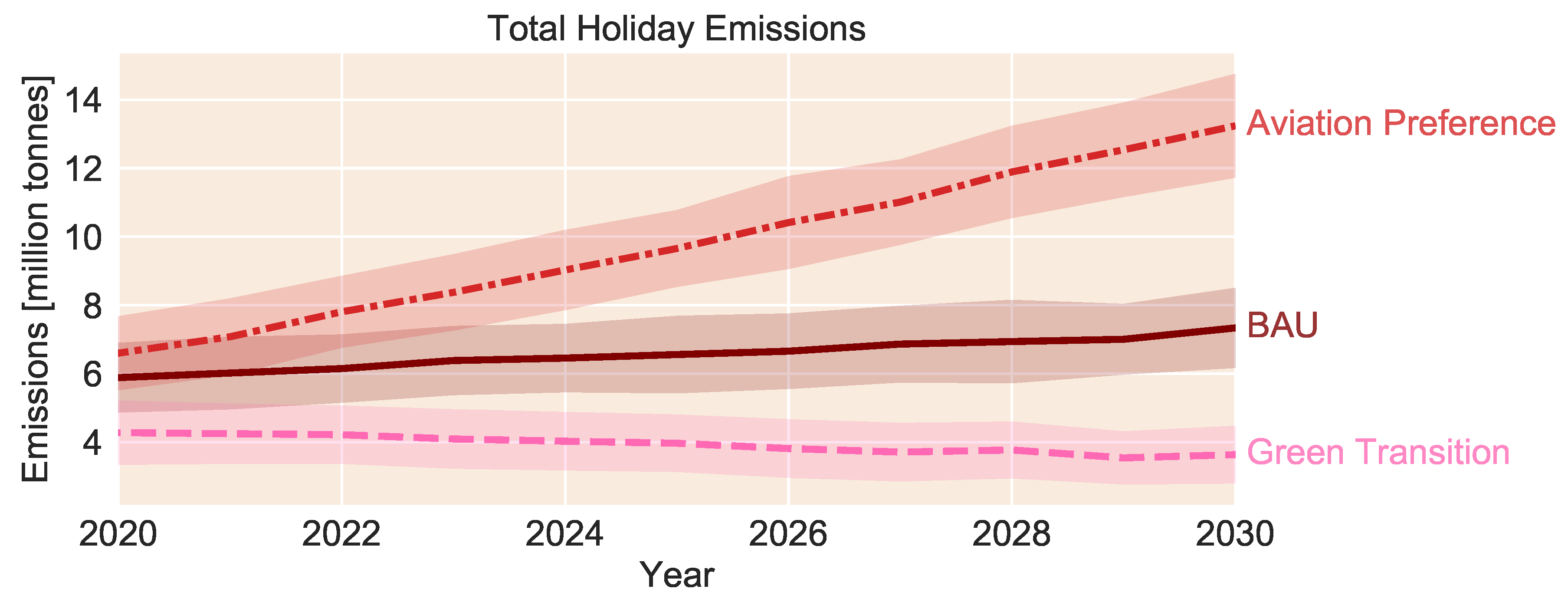
In the case of air travel, the increases in emissions are counter-proportional (Figure 12), so that ‘Aviation Preference’ has a strong increase in emissions, in the case of the ‘Green Transition’ to an emission drop that changes into a constant emission level can not be further reduced under this. The total emissions (Figure 13) correspond strongly to the trends of the aviation sector which produces by far the largest amount of emissions while being the minority in terms of overall trips.

6. Discussion

The decision to go on a holiday and the choice of destination are not primarily driven by financial deliberations. This is why purely economic models only show a small part of the bigger picture and resulting predictions may be flawed. This issue becomes even more crucial, if we expect a change in behaviour or social norms in the near future. In order to close this research gap, we designed a social simulation concept to capture emergent aspects of social changes, giving rise to several trends in holiday demand. Thus, the presented decision-making on holiday travel considers social bonding as well as financial aspects, though the latter is implemented as a rather simplistic scheme, which was sufficient for our purpose. With this, we were able to reconstruct empirical data of Austrian tourism behaviour over the time span of more than a decade in great detail.

Another advantage of the model is the individual-based resolution of decisions. With this method, we were able to estimate the CO₂ footprint of short and long distance travel and capture shifts in trends between land and air transport as well as domestic and international travel.

The standard approach to estimate country-based aviation emissions is based on national sold kerosene [Environment agency Austria—Report 2019]. However, this method can only be compared with our results to a limited extent, as we calculate the CO₂ contribution of Austrian residents and fuel sales reflect the activities of Austrian Airports. In comparison, the here-presented footprint of Austrian holiday travel activities in 2018 of 4.39 kg is significantly higher than that of the official report with 2.61 million tons of air traffic in Austria in 2018 [1,20]. We believe several factors accentuate the difference between our model results and other approaches to calculate aviation emissions:

Refuelling and transferring to other aircraft plays an enormous role in this context. We argue that domestic kerosene sales do not take any account of the fact that most long-distance travel include stopovers that take place at transshipment airports. In view of this, there is an extreme distortion between the footprint of individual travel and national kerosene sales.
International flight emissions per 100 km are reported to be 41.49 kg [21]. The result for our model is 21.1 kg per 100 km flight distance due to the use of TREMOD, a suitable emission model explained in detail in Appendix A.1.1. Thus, the emission factor applied by us is clearly lower than the value quantified by the Environment Agency Austria. There are various reasons for this discrepancy that are related to how emissions are calculated. Using the kerosene sold in a country as a starting point leads to different results than calculating how much kerosene is needed to transport individuals to their chosen destinations and back. The global sum of both approaches should be identical, but when trying to find out which country is responsible for the emissions, there is a significant difference, especially for smaller countries.
We have not investigated flight-based emissions stemming from flight movement statistics.

In regard to land travel, we compare emission factors used in our model and the official report of the Environment Agency Austria (EAA) [21]:

Car travel emission factors per person in TREMOD are 9.5 kg (2 person occupancy) compared to the EAA amount of 22.7 kg (1.15 person occupancy) for 100 km.
Train travel emission factors per person in TREMOD are 3.6 kg compared to the EAA amount of 1.44 kg in 100 km.
Bus travel emission factors per person in TREMOD are 2.3 kg compared to the EAA amount 5.79 kg in 100 km.

With this model being a starting point of our investigation, several simplifications were made for a first estimation of emission calculation. Route related aspects such as city-to-city distances or intermediate stops (especially relevant for flight related emissions) have not been accounted for. Moreover, different vehicle types (age, size and fuel type) and their correlated emissions, traffic jams, different land distances for train travel than car routes, detours and other deviations are not taken into account. Additionally, the used data set did not contain detailed information about the distribution of transport modes used to reach a certain country, so these distributions had to be approximated and calibrated.

The scope of the presented model is not limited to Austria. In principle, it can be used for any country but since Austria is a landlocked country, many regions would necessitate an extension to water routes. The model requires the number of residents and the ratio between land and air travel. If the latter is not available, it is possible to approximate these values with the values obtained for Austria, scaled to the population of the analysed country and its GDP. At least for other European countries, this should give a useful approximation, although such a process would naturally decrease the accuracy of the model. However, even with decreased accuracy, the model could still be used to compare different scenarios, which can provide policy recommendations for an arbitrary country.

For future research, we are interested in implementing more detailed travel routes. So far, our estimation is based on mean distances, however statistics on start-to-end travel distances would be useful to implement for land routes. In terms of flight emissions, start-to-end travel statistics can than be combined with airport-to-airport distances (https://www.world-airport-codes.com/) to enhance the emission calculation. Additionally, it would be interesting to implement train routes for a more accurate estimation of the correlated emissions. For the social simulation, we intent to include more social-psychological aspects such as habits (preferred travel destinations) and more detailed options in decision making regarding financial spending for car, bus and train as well a different interaction mechanism that accounts for persuasion.

7. Conclusions

The presented model on holiday travel behaviour of Austrian residents (above 15 years old) was used to calculate the number of domestic and international trips for land and air travel in the period 2003–2030. Moreover, we calculated CO₂ emissions of holiday travel activities and showed three scenarios for future trends. The main results are:

On average, a single domestic trip (both ways) produces 29.3 kg of CO₂, a single international trip by land 131 kg and a single international trip by air 1260 kg, resulting in an approximate ratio of 1:4.5:43 in average emissions production (reference year 2016).
In total, domestic travel produced 290965 tonnes of CO₂, international road travel 907628 tonnes and international flights 4159355 tonnes. This leads to a ratio of 1:3.1:14. The reduction in the share of total air travel compared to average single trips relates to the smaller contingent of air travel of 15.8% in 2016.
The impact of travel traffic emissions has been rising continuously since 2003. In that year, total travel emissions amounted to 3.8 million tonnes, in 2018 to 5.8 million tonnes. For business as usual, an increase to more than 7.3 million tonnes is probable by 2030.
Not only has the total number of trips increased since 2003, but the share of air travel has also increased from 12.5 % (2003) to 16.2% (2019) and will rise to 19.4% (2030) in about ten years if the current trend continues.
Further increase in annual emissions could be halted through a green transition, which includes a price increase on airline tickets compared to other transportation options, a decrease in long-distance flights and additionally promoting land trips. The proportion of air travel could fall to 9.5% by 2030 and bring total emissions to 3.6 million tonnes, a level similar to 2003.
A maladaptation to the current emissions problem through further increases in air travel, especially enhanced trends towards more long-distance travel, could lead to an immense increase in annual emissions of up to 13.2 million tonnes in 2030.

A further discussion of the results in relation to other estimates of emissions and prospects to decrease transportation related emissions includes the following:

Annual Austrian holiday travel demand air emissions are almost double as high as aviation emissions based on Austria’s sold kerosene. This mismatch is likely due to intermediate stops of long-distance flights and transfer to other aeroplanes which nationally sold fuels cannot account for.
Austrian holiday aviation contributed with 0.5% to the worldwide civil aviation of 895 million tonnes of CO₂ in 2018.
Since our results are based on direct flights, including detours and intermediate stops in air travel routes would lead to even higher annual aviation emission estimations.
Reducing emissions is possible by increasing the share of domestic holidays, which would benefit local business and the Austrian economy. Since the average Austrian goes on a holiday 3.5 times a year, a reduction for the second or third domestic trip (i.a. hotel booking in Austria) would be conceivable. General incentives for domestic travel would be feasible to tackle this issue.
The land emissions presented here are based on medium-sized and medium-aged petrol-powered vehicles producing 9.5kg CO₂ emissions in 100 km. A green transition towards less emissions is facilitated by electric cars (4.8 kg), modern and small petrol-based cars (7.4 kg), hybrid cars (6.1 kg). The trend towards large petrol-based cars such as SUV (12kg) would increase the estimated land emissions by up to 26%.
The share of bus and train that turned to air travel in the 1980s need to be reverted for a green movement. To achieve this, Europe-wide public transport needs to be improved in terms of service, availability, comfort and on time departure. We estimate that this could reduce annual CO₂ emissions from holiday travel by 20%.
Projections of the aviation industry’s share of global emissions include a rise to 22% by 2050 if no new radical technologies or policies are introduced [22]. With this being a projection of the business-as-usual, we want to add to this discussion the possible risk of social norm shifts towards more aviation and especially an increase in long-distance luxury destinations that could double the projected increase. However, due to limited technological efficiency potentials, it is unlikely to meet the predicted increases in demand [23].

Author Contributions

Conceptualisation, M.L.K. and G.J.; methodology, M.L.K. and G.J.; software, M.L.K.; validation, M.L.K.; formal analysis, M.L.K.; investigation, M.L.K.; data curation, M.L.K.; writing–original draft preparation, M.L.K.; writing–review and editing, M.L.K. and G.J.; visualisation, M.L.K.; supervision, M.F.

Funding

M.L.K. receives a student grant by Steiermärkische Sparkassen and the University of Graz, Austria. Open Access Funding by the University of Graz.

Conflicts of Interest

The authors declare no conflict of interest. The funders had no role in the design of the study; in the collection, analyses, or interpretation of data; in the writing of the manuscript, or in the decision to publish the results.

Abbreviations

The following abbreviations are used in this manuscript:

ABM	Agent Based Model
BAU	Business-As-Usual
CO₂	Carbon Dioxide
CO₂eq	Carbon Dioxide Equivalents
EAA	Environment Agency Austria
GHG	Greenhouse Gases
IPCC	Intergovernmental Panel on Climate Change
TREMOD	Transport Emission Model
STD	Standard Deviation

Appendix A. Materials and Methods

This section provides further details about the empirical data sets and an extensive insight into the model structure.

Appendix A.1. Empirical Information

Travel behaviour of the Austrian population is provided by Statistics Austria [6,8]. The survey scheme is in accordance with EU regulations on tourism statistics, details on survey methods are available in the standard documentation of travel behaviour of the Austrian population [7]. The collected data are quarterly reports of computer assisted telephone interviews, the sample size is 3500 people of Austrian residents above the age of 15 years. Considered holiday travels have at least one overnight stay. Our main interest in empirical data are number of tourists and trips per year, top destinations, amount of personal and professional travels, transport vehicle and holiday destination choices. All data required for our application is presented in Table 1, Table 2, Table 3, Table 4 and Table 5.

As complementary travel data source we used the Eurostat (statistical office of the European Union) online publication [24] which provides annual statistical data on tourism demand in the European Union.

TREMOD—Transport Emission Model

The Transport Emission Model TREMOD is the calculation basis for route-based CO₂ emissions in the here presented research [25]. This model was developed for motorised traffic in Germany, which makes it highly suitable for the Austrian equivalent. The model covers diverse human-made greenhouse gases in respect to transportation modes. The calculated emissions capture the functionally equivalent amount of concentration of carbon dioxide CO₂eq, which to simplify matters, we refer to as CO₂. TREMOD takes into account exhaust emissions from fuel combustion and emissions in the “well-to-wheels” chain. Emissions resulting from the manufacture and disposal of means of transport and for the infrastructure required, e.g., for roads, are not considered. We use standard parameters for the car transportation:

6.8

L/km (petrol), middle sized and middle aged car type. An online implementation of TREMOD is available at https://www.quarks.de/umwelt/klimawandel/co2-rechner-fuer-auto-flugzeug-und-co/ (German only).

Appendix A.2. Model: Agent-Based Decision Modelling

Holiday travel decisions are investigated by an agent-based model (ABM) which we implemented in Netlogo 6.0.4. The model consists of a population of 1000 agents that can make several holiday travel decision in a single round. Each round represents a year, thus successive rounds can be used to examine trends. Agents have their individual wealth—and associated travel budget—and their own preferences towards land or air travel. Agents are interconnected with other agents who represent their potential travel partners. The implemented topology is a spatial-proximity network, representing likely connections in their own region to simulate real-life interactions [26]. The resulting network topology serves as a friendship network for agents to find others that they wish to travel with, which is a necessity for the actual holiday choice.

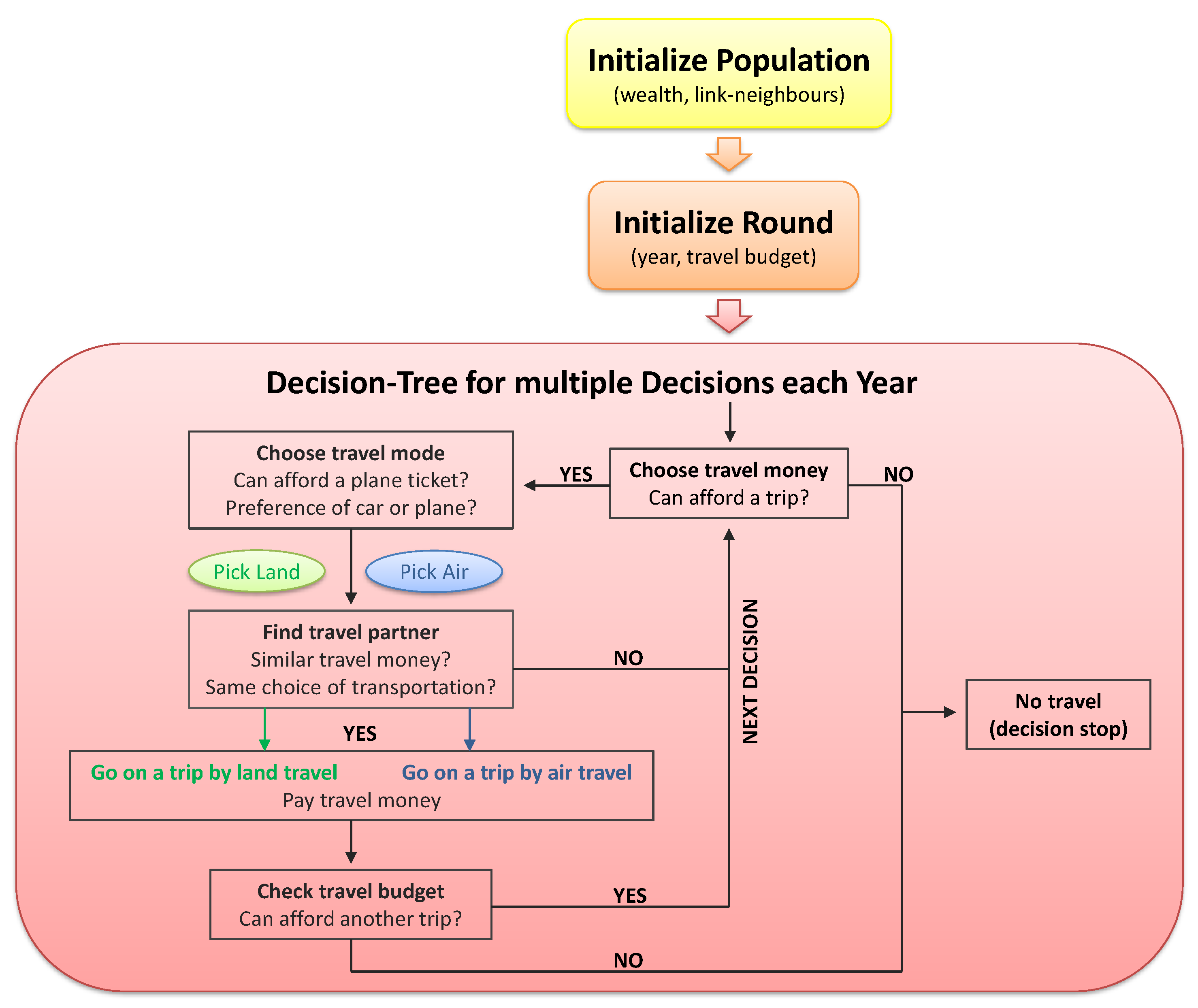
Figure A1. Decision tree for Agent-based decision modelling: initialisation (yellow and orange boxes) are followed by a decision process to capture each decisions expenditure, travel mode and companionship to either decide to go on a travel or not for multiple decisions per year.

Appendix A.2.1. Decision Tree

The mechanism to reach a decision is divided into several sub-decisions, given by a decision-tree, see Figure A1. Starting a simulation run, all agents and their friendship links are created (yellow box). Each agent receives an individual wealth W and the network topology is generated. Both features remain constant after initialisation. Secondly, agents receive a preference to travel by car

P_{c}

which can be adjusted for different scenarios.

The time evolution is given in rounds, a single round is related to one year of holiday travel decisions. At the beginning of each round, agent’s travel budgets B for this year are determined according to their wealth (orange box). During one year, agents have several decisions to make (red box) until their travel budget is exhausted. Each decision process starts with checking the current travel budget. If a trip can be afforded, agents decide on the transportation mode. Afterwards, agents check their network neighbours’ choices in regard to their travel money and whether they chose air or land travel. If they find a travel partner with similar preferences, they decide to go on a trip, otherwise they decide not to travel. This decision process is repeated several times each round so that agents can go on several trips per year.

Appendix A.2.2. Transportation Choice

The choice of transportation is given by monetary and personal constrains or preferences. Monetary constrains are implemented by air travel pricing. Assuming a simple equilibrium pricing, ticket prices are evenly distributed and the maximal possible ticket price is equal to the maximal possible travel budget, which can be spend on a ticket. Deviation from the equilibrium pricing such as increasing air ticket prices poses a constrain. On the other hand, decreasing it gives an incentive for agents to choose air travel. All financial aspects are implemented in generic monetary units such that only their relative value is important for the decision process. Thus, changes in air ticket prices simply result in an advantage or disadvantages over land travel.

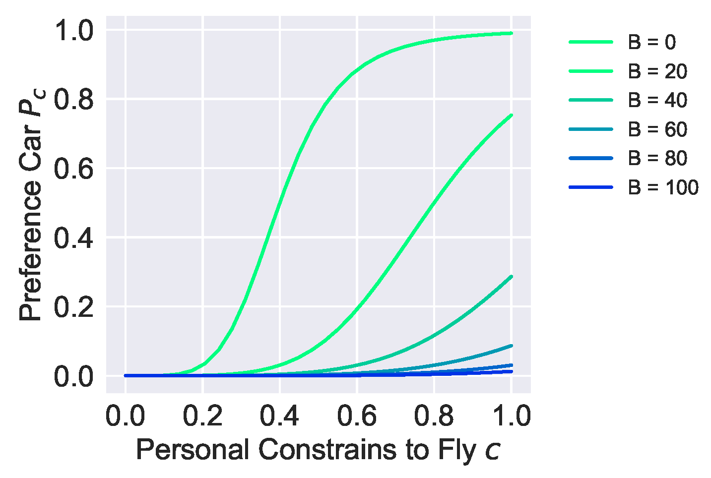
Personal constrains evolve around preferences between land travel and air travel. We use the terminology of constrain to emphasise that air travel is much less common than land travel due to several reasons such as aversion, fear and environmental concerns, but this notion also includes habits and cultural aspects. To model transport preferences, we use a preference probability for land travel

P_{c}

defined by the Hill function, which is commonly used to model density dependent growth or decline. We use a simple version of the Hill function given by the equation

P_{c} = \frac{x^{λ}}{h^{λ} + x^{λ}} .

(A1)

The preference probability

P_{c} \in [0, 1]

is mediated by agent’s personal constrain

c \in [0, 1]

and their budget

B \in [0, 100]

. Relating the hill function to model parameters therefore holds

\begin{matrix} x & = c \end{matrix}

(A2)

\begin{matrix} h & = 2 B / 100 + h_{f} . \end{matrix}

(A3)

and is shown in Figure A2 for

h_{f} = 0.4

six different travel budgets. Note that the factor

h_{f}

is used to shift the preference probability in different scenarios with

h_{f} = 0.4

(BAU),

h_{f} = 0.2

(Green Transition), and

h_{f} = 0.6

(Aviation Preference) which holds a small differences in the collective preferences towards air or land travel. The population mean of the personal constrain to fly is always at

C = 0.5 \pm 0.1

.

Figure A2. Preference probability for car travel

P_{c}

for each agent personal constrain to fly c and current budget B.

Figure A2. Preference probability for car travel

P_{c}

for each agent personal constrain to fly c and current budget B.

Appendix A.2.3. ABM Settings

Agent-based model parameters and configurations for the reference year 2016 and trends over longer time spans are shown in Table A1. The empirical information as presented in Section 2 is used for the Austrian population factor, which relates the model output to the number of Austrian residents in the respective year. The maximal number of decisions per year is in accordance to annual Austrian vacation days. The mean population wealth and mean standard deviation (STD) of population wealth are in accordance to Figure 1. The monetary thresholds gives the minimal budget necessary to engage into any further travels. The maximal wealth and correlated annual budget and travel money as well as air ticket prices are given in generic monetary units. Other parameters (node degree, annual wealth increase, hill parameter) are used to match the empiric data. The chosen combination of these parameters has proved useful to show the trend over the period 2003–2030. However, other parameter combinations are possible, as the model is not particularly sensitive to changes. For example, similar results are given for a more strongly connected social network and lower number of maximum decisions, since this case corresponds to the formation of large travel groups. Also, parameters regarding ticket prices or wealth growth can be varied widely. The main critical setting is the division of the travel money into one third of the agent’s annual budget, otherwise the agents are likely to spend too much on a single travel and therefore engage in less trips overall.

Table A1. Agent-based model parameters and configurations for the reference year 2016 and trends. Agent’s individual parameters are denoted with an index i. External predefined parameters are highlighted in bold.

ABM Settings
External Parameter	Reference Year (2016)	Trends/Scenarios
Year	2016	2003–2030
Austria population factor	7372000	6676000–8112100
Max. decisions per year	9
Mean population wealth	29.24	acc. to wealth increase
STD Population wealth	19.62
General Settings
Agents	1000
Network Topology	Spatial Proximity
Wealth $W_{i}$	$\in [0, 100]$
Annual budget $B_{i}$	$\in [0, W_{i}]$
Travel money	$\in [0, B_{i} / 3]$
Air ticket price	$\in [0, 100]$ (BAU)	$+ 2.5 /$ a (aviation), $- 2.5 /$ a (green)
Monetary threshold	$< 5$
Population mean air travel constrain	$0.5 \pm 0.1$
Fitted Parameter
Hill Parameter	$0.4$ (BAU)	$0.2$ (green), $0.6$ (aviation)
Annual wealth increase	0	$\pm 0.48$ a
Network avg. node degree	3

Appendix A.3. Model: Emission Calculation

The presented emission calculation model is implemented in Python 3.6. Figure A3 shows the scheme of the emission calculation which was used for normal trend evaluation and all scenarios. The input data of the ABM are total trips, total land and total air travel. With inbound and outbound travel being about equally frequent since the year 2003, we assume equal shares of domestic and international trips. Half of the trips are used to calculate inbound travel (land only), while half of the trips are used for outbound travel (land and air). For inbound travel, the trip destination assignment evolves for each trip according to Table 4. For outbound travel, each trip is assigned an international destination according to Table 5. A country-based land-air ratio holds the probability for each trip to be land or air travel. Based on this procedure, we calculate the sum of all travel routes to estimate yearly travel behaviour.

Figure A3. Emission Calculation Scheme: Using ABM generated data on travel amounts as input, the model performs a trip destination assignment for domestic and international travel destinations and calculates the corresponding emissions in relation to land and air travel modes.

In the last step, emission calculation is based on distance-related data stemming from TREMOD transport emission calculation. Emission calculation is based on the doubled amount of trips to account for the return journey. For different land travel options, the default share of train and bus travel is 18% since the relative ratio of passenger cars to public transport has been relatively constant over the last years for both domestic and international travel. For the scenarios ‘green transition’ and ‘aviation preference’ this ratio is shifted to 25% and 12% respectively.

Appendix A.4. Land-Air Ratio

For inbound travel, we assume a

100 / 0

land-air ratio, which reflects the statistical information of land travel being about

99.7 %

. However, for international travel the relation between land and air travel (LA-ration) is more complex since it is subservient to the annual changing share of total air travel, and as well depending on country-based diversities.

While most parts of the model can be compared to empirical data provided by Statistics Austria, the individual ratio between land travel and air travel for each country is not available. With this being a missing piece of information, it is necessary to make assumptions about country-based land-air ratios

L C

. To approximate the land-air ratio of different destinations, we divide countries and ratios into four groups:

(i): For directly neighbouring countries (e.g., Germany, Italy) we assume mostly land travel and a land-air ratio of $95 / 5$ $(L C = 95)$ .
(ii): Countries with travel distance shorter than 1200 km are assigned a land-air ratio of $70 / 30$ $(L C = 70)$ .
(iii): Countries with travel distance longer than 1200 km up to 3000 km are assigned a $30 / 70$ $(L C = 30)$ ratio.
(iv): Countries with distance >3000 km or those who cannot be reached without directly passing a water way are in the last category of $0 / 100$ $(L C = 0)$ land-air travel, which means that they are only travel to by air.

With this categorisation we can exemplary calculate the modelled total land-air ratio of international travel. Supposing there are large contingent of outbound trips. Using the presented country-based ratios, the modelled share of outbound land travel is

65.3 %

and outbound air travel of

L A = 34.7 %

, which we refer to as the LA-factor. Comparing these results to the empirical data of the reference year 2016 with

65.7 %

land and

34.4 %

air travel, we can use the presented calculation as a baseline for our estimation of travel choices per country.

Second, we have to account for trends in the total land-air ratio of outbound travel. On the assumption that one year shows a lower (or higher) share of air travel than the reference year, the country-based ratio

L C

need to be shifted accordingly. To do this, we correlate the LA-factor of the decision-based model

L A_{a b m}

with the country-based ratios

L C = [95, 70, 30]

by adopting a simple linear shift

L C_{t r e n d} = L C + a * (L A - L A_{a b m})

(A4)

with a being a positive constant value. Due to the adjusted

L C_{t r e n d}

, different proportions of land and air travel can now be included in the emission calculation. Due to different trends in the future projections, we use

a = 1

for the BAU trend,

a = 0.5

for the ‘Green Transition’ scenario and

a = 0.9

for the ‘Aviation Preference’ scenario.

Furthermore, preferences in destinations can manifest themselves differently with proper policies or social norm processes (going green). We are accounting for preference shifts in aviation destinations by limiting (Green Transition) or extending (Aviation Preference) the amount of minor destinations. Since these destination share contains mainly luxury destinations like Fiji Islands, Argentina or New Zealand, we implement a preference adjustment by implementing a luxury preference factor

P_{L} = L A - L A_{a b m}

. Here, positive

P_{L}

decrease the number of luxury travels while negative

P_{L}

increase this destination share. For example, if

P_{L} = 0.1

an initial share of luxury destinations of

18 %

is decreased to

17.4 %

. Deviations between air travel of the AMB and trip assignment of the emission calculation model are minor with the mean deviation being

0.285

(BAU),

0.98

(Green Transition), and

0.53

(Aviation Preference) for each scenario respectively.

To summarise, due to the adjusted

L C_{t r e n d}

, different proportions of outbound land and air travel can be used for the emission calculation of the scenarios BAU, ‘Green Transition’ and ‘Aviation Preference’.

Distances

Excluding countries from land travel is based on two assumptions: on the one hand, on the huge distances from Austria to the corresponding country (e.g., China), and on the other hand on cutting off the direct route through the oceans. The latter assumption stems from statistical data regarding the choice of means of transport which shows that ship transport is insignificantly small (0.2%). Thus, we assume pure air transport for travel distances

> 3000

km and destinations routes passing water ways.

We use different methods to calculate distances for land and air travel. Land travel distances are based on road information, which are accessed via Google maps [27]. Air travel distances are the shortest paths (linear distance or bee-line) between Austria and the respective country. All estimates are based on the centre of each country, both for Austria and for the destination country. Exceptions to this rule are given when a destination record sums up several countries, e.g., ‘other American countries’. For this cases we use the mean of the top six holiday destinations of the respective region.

References

Juvyns, O.; Fernandez, R.; Mandl, N.; Rigler, E. Annual European Union Greenhouse Gas Inventory 1990–2017 and Inventory Report 2019; Technical report; European Commission, DG Climate Action European Environment Agency: Brussels, Belgium, 2019. [Google Scholar]
Turner, R.; Jus, N. Travel & Tourism: Economic Impact 2019; Technical Report; World Travel & Tourism Council (WTTC): London, UK, 2019. [Google Scholar]
Peeters, P.; Szimba, E.; Duijnisveld, M. Major environmental impacts of European tourist transport. J. Transp. Geogr. 2007, 15, 83–93. [Google Scholar] [CrossRef]
Knowles, R.D. Transport shaping space: Differential collapse in time–space. J. Transp. Geogr. 2006, 14, 407–425. [Google Scholar] [CrossRef]
International Air Transport Association. IATA 20-Year Air Passenger Forecast; IATA: Montreal, QC, Canada, 2015. [Google Scholar]
Laimer, P.; Lebersorger, S. Urlaubs- und Geschäftsreisen Kalenderjahr 2016; Technical Report; Statistics Austria: Vienna, Austria, 2017.
Laimer, P.; Ostertag-Sydler, J. Standard-Dokumentation Metainformationen zu Reisegewohnheiten der österreichischen Bevöökerung; Technical report; Statistics Austria: Vienna, Austria, 2017.
Wurian, R. Urlaubs- und Geschäftsreisen Kalenderjahr 2018; Technical report; Statistics Austria: Vienna, Austria, 2019.
Fessler, P.; Lindner, P.; Schürz, M. Eurosystem Household Finance and Consumption Survey 2017; Technical report; Oesterreichische Nationalbank: Wien-Alsergrund, Austria, 2019. [Google Scholar]
Kulczyk-Dynowska, A.; Bal-Domańska, B. The National Parks in the Context of Tourist Function Development in Territorially Linked Municipalities in Poland. Sustainability 2019, 11, 1996. [Google Scholar] [CrossRef]
Poterba, J.M. Tax Policy to Combat Global Warming: On Designing a Carbon Tax; Technical report; National Bureau of Economic Research: Cambridge, MA, USA, 1991. [Google Scholar]
Pearce, D. The role of carbon taxes in adjusting to global warming. Econ. J. 1991, 101, 938–948. [Google Scholar] [CrossRef]
Agostini, P.; Botteon, M.; Carraro, C. A carbon tax to reduce CO2 emissions in Europe. Energy Econ. 1992, 14, 279–290. [Google Scholar] [CrossRef]
Tol, R.S. The impact of a carbon tax on international tourism. Transp. Res. Part Transp. Environ. 2007, 12, 129–142. [Google Scholar] [CrossRef]
Anger, A. Including aviation in the European emissions trading scheme: Impacts on the industry, CO₂ emissions and macroeconomic activity in the EU. J. Air Transp. Manag. 2010, 16, 100–105. [Google Scholar] [CrossRef]
Krenek, A.; Schratzenstaller, M. Sustainability-oriented tax-based own resources for the European Union: a European carbon-based flight ticket tax. Empirica 2017, 44, 665–686. [Google Scholar] [CrossRef]
Graham, B.; Shaw, J. Low-cost airlines in Europe: Reconciling liberalization and sustainability. Geoforum 2008, 39, 1439–1451. [Google Scholar] [CrossRef]
Dobruszkes, F. New Europe, new low-cost air services. J. Transp. Geogr. 2009, 17, 423–432. [Google Scholar] [CrossRef]
De Wit, J.G.; Zuidberg, J. The growth limits of the low cost carrier model. J. Air Transp. Manag. 2012, 21, 17–23. [Google Scholar] [CrossRef]
VCÖ. Kurzbericht Entwicklung Kerosinverbrauch und CO2-Emissionen des Flugverkehrs in Österreich; Technical report; VCÖ Verkehrsclub Österreich: Vienna, Austria, 2019. [Google Scholar]
Umweltbundesamt Österreich. Emissionskennzahlen Datenbasis 2017. Available online: https://www.umweltbundesamt.at/fileadmin/site/umweltthemen/verkehr/1_verkehrsmittel/EKZ_Pkm_Tkm_Verkehrsmittel.pdf (accessed on 7 October 2019).
Cames, M.; Graichen, J.; Siemons, A.; Cook, V. Emission reduction targets for international aviation and shipping. In Directorate General for Internal Policies; European Parliament—Policy Department A; Economic and Scientific Policy: Bruxelles, Belgium, 2015. [Google Scholar]
Bows-Larkin, A. All adrift: Aviation, shipping, and climate change policy. Clim. Policy 2015, 15, 681–702. [Google Scholar] [CrossRef]
EUROSTAT. Annual Data on Trips of EU Residents (tour_dem). 2019. Available online: https://ec.europa.eu/eurostat/web/tourism/data/database (accessed on 7 October 2019).
Knörr, W.; Höpfner, U. TREMOD—Schadstoffe aus dem motorisierten Verkehr in Deutschland. In 20 Jahre ifeu-Institut; Springer: Heidelberg, Germany, 1998; pp. 115–128. [Google Scholar]
Stonedahl, F.; Wilensky, U. NetLogo Virus on a Network Model; Center for Connected Learning and Computer-Based Modeling, Northwestern University: Evanston, IL, USA, 2008. [Google Scholar]
Google. Google Maps Directions for Driving from Austria to National and International Destinations. 2019. Available online: https://maps.google.com (accessed on 11 September 2019).

Figure 1. Economic spending behaviour: Perceived wealth of individuals by self-assessment in regard to their own position in the wealth distribution based on data sets of the 2014 and 2017 Eurosystem Household Finance and Consumption Survey. In the model, a continuous function is needed. It was obtained by fitting a Gaussian distribution to the available data, which resulted in

μ = 3.924

and

σ = 1.962

.

Figure 1. Economic spending behaviour: Perceived wealth of individuals by self-assessment in regard to their own position in the wealth distribution based on data sets of the 2014 and 2017 Eurosystem Household Finance and Consumption Survey. In the model, a continuous function is needed. It was obtained by fitting a Gaussian distribution to the available data, which resulted in

μ = 3.924

and

σ = 1.962

.

Figure 2. Holiday demand trend analysis: Historical data and future scenario of business-as-usual. Yearly information of amount of tourists (grey), total number of trips (orange), total number of land travel (green), and total number of air travel (blue) is shown for the period 2003–2030. Empirical data (dots) and linear trend fitting (line) is compared to model data (dashed line). Shaded areas show a 10% deviation from empirical average values.

Figure 3. Proportions of Land and Air Travel for business-as-usual shown for domestic and international destinations from 2003–2030.

Figure 4. Holiday demand travel emissions in the period 2003–2030: Annual average emissions from holiday travel shown for the business-as-usual ‘BAU’ trend for land travel (green), air travel (blue) and total travel (red).

Figure 5. Future trends for land travel: mean number of (left) domestic and (right) international are shown for three scenarios BAU —business as usual (solid line), ‘Green Transition’ (dashed line), and ‘Aviation Preference’ (dashed-dotted line) and estimated model errors (shaded areas). The number of trips is given in kilo trips [k].

Figure 6. Future trends for land travel: land travel (domestic and international combined) means are shown for three scenarios BAU—business as usual (solid line), ‘Green Transition’ (dashed line), and ‘Aviation Preference’ (dashed-dotted line) and estimated model errors (shaded areas). The number of trips is given in kilo trips [k].

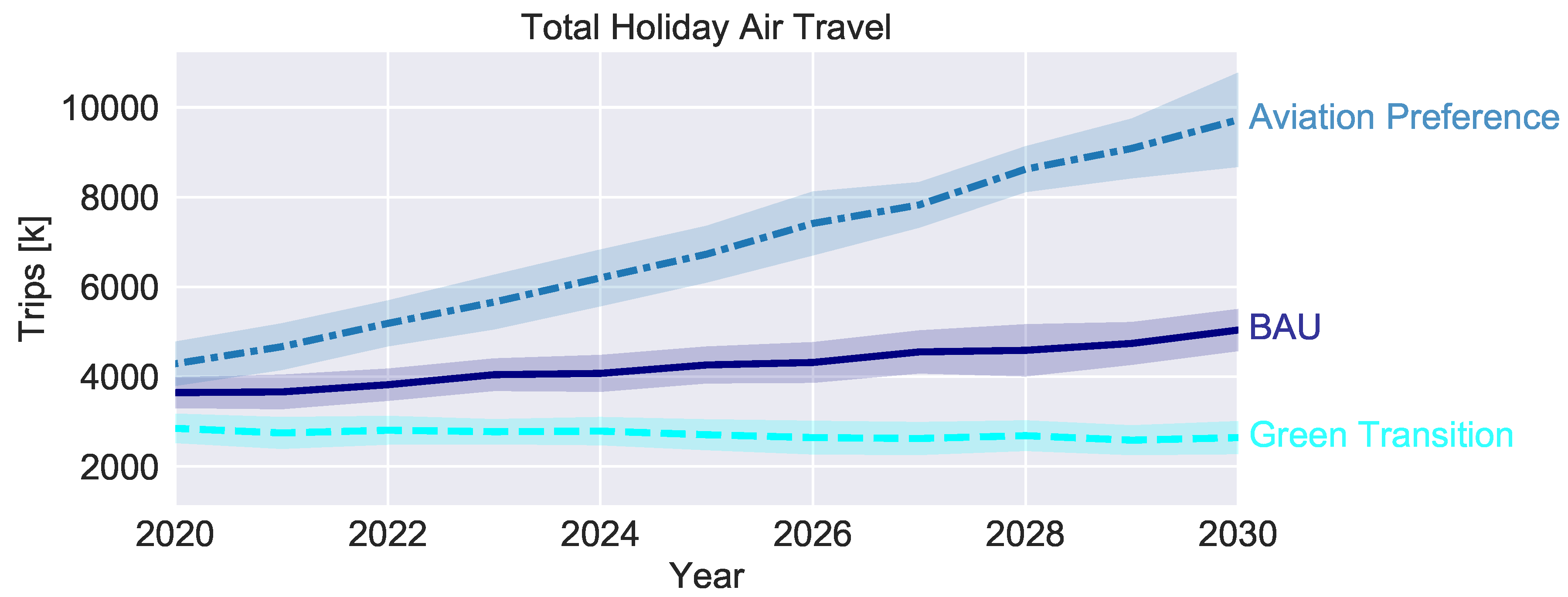
Figure 7. Future trends for air travel: air travel (international) means are shown for three scenarios BAU—business as usual (solid line), ‘Green Transition’ (dashed line), and ‘Aviation Preference’ (dashed-dotted line) and estimated model errors (shaded areas). The number of trips is given in kilo trips [k].

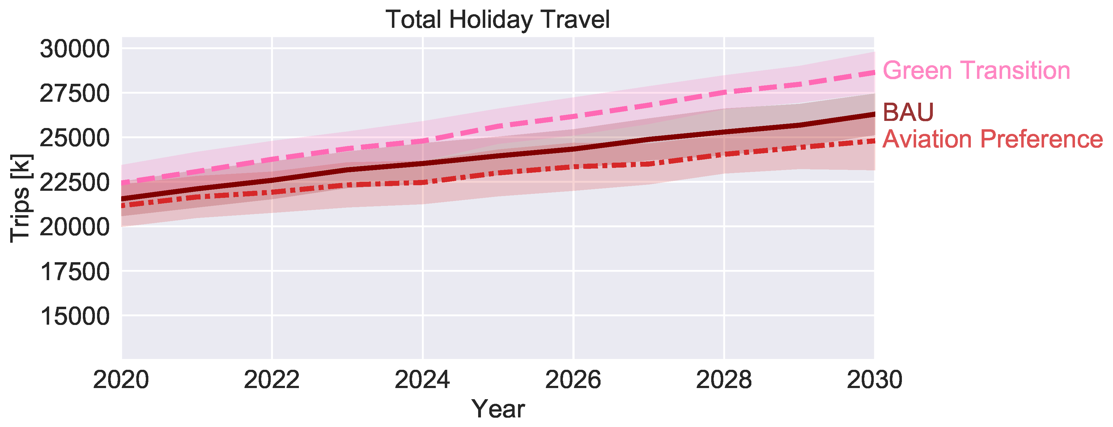
Figure 8. Future trends for holiday travel: all travel (domestic and international combined) means are shown for three scenarios BAU—business as usual (solid line), ‘Green Transition’ (dashed line), and ‘Aviation Preference’ (dashed-dotted line) and estimated model errors (shaded areas). The number of trips is given in kilo trips [k].

Figure 9. Future projections of the proportions of Land and Air Travel for the scenarios (top) ‘Green Transition’ and (bottom) ‘Aviation Preference’ in the period 2020–2030.

Figure 10. Future CO₂ emissions trends for land travel: mean amount of (left) domestic and (right) international are shown for three scenarios BAU—business as usual (solid line), ‘Green Transition’ (dashed line), and ‘Aviation Preference’ (dashed-dotted line) and estimated model errors (shaded areas); emissions are given in

10^{9}

kg [million tonnes].

Figure 10. Future CO₂ emissions trends for land travel: mean amount of (left) domestic and (right) international are shown for three scenarios BAU—business as usual (solid line), ‘Green Transition’ (dashed line), and ‘Aviation Preference’ (dashed-dotted line) and estimated model errors (shaded areas); emissions are given in

10^{9}

kg [million tonnes].

Figure 11. Future CO₂ emissions trends for land travel: mean amount of land travel (domestic and international combined) is shown for three scenarios BAU—business as usual (solid line), ‘Green Transition’ (dashed line), and ‘Aviation Preference’ (dashed-dotted line) and estimated model errors (shaded areas); emissions are given in

10^{9}

kg [million tonnes].

Figure 11. Future CO₂ emissions trends for land travel: mean amount of land travel (domestic and international combined) is shown for three scenarios BAU—business as usual (solid line), ‘Green Transition’ (dashed line), and ‘Aviation Preference’ (dashed-dotted line) and estimated model errors (shaded areas); emissions are given in

10^{9}

kg [million tonnes].

Figure 12. Future CO₂ emissions trends for land travel: mean amount of international air travel is shown for three scenarios BAU—business as usual (solid line), ‘Green Transition’ (dashed line), and ‘Aviation Preference’ (dashed-dotted line) and estimated model errors (shaded areas); emissions are given in

10^{9}

kg [million tonnes].

Figure 12. Future CO₂ emissions trends for land travel: mean amount of international air travel is shown for three scenarios BAU—business as usual (solid line), ‘Green Transition’ (dashed line), and ‘Aviation Preference’ (dashed-dotted line) and estimated model errors (shaded areas); emissions are given in

10^{9}

kg [million tonnes].

Figure 13. Future CO₂ emissions trends for holiday travel: mean amount of total emissions (domestic and international) is shown for three scenarios BAU—business as usual (solid line), ‘Green Transition’ (dashed line), and ‘Aviation Preference’ (dashed-dotted line) and estimated model errors (shaded areas); emissions are given in

10^{9}

kg [million tonnes].

Figure 13. Future CO₂ emissions trends for holiday travel: mean amount of total emissions (domestic and international) is shown for three scenarios BAU—business as usual (solid line), ‘Green Transition’ (dashed line), and ‘Aviation Preference’ (dashed-dotted line) and estimated model errors (shaded areas); emissions are given in

10^{9}

kg [million tonnes].

Table 1. Empirical data of tourism trips of Austrian residents in 2016. (Left) total trips, (mid) holiday trips for personal reasons and (right) business trips for professional reasons. Data Source: [6].

Statistical Data on Tourism Demand of Austrians in 2016
	Total Trips [k]	Holiday Trips [k]	Business Trips [k]
All Destinations	23561	19683	3878
Inbound	12026	10063	1963
Land Travel	11965	10030	1934
Air Travel	58134	28	29
Outbound	11534	9619	1915
Land Travel	7134	6280	855
Air Travel	4358	3300	1059

Table 2. Empirical data of tourism transportation mode for holiday travel of Austrian residents from 2016. Train and bus transportation is shown combined as “Other.” Data Source: [6].

Statistical Data on Holiday
Transportation Choices of Austrians in 2016
	Total	Inbound	Outbound
Land	$83.1 %$	$99.7 %$	$65.7 %$
Car	$64.8 %$	$80.1 %$	$48.8 %$
Other	$18.2 %$	$19.5 %$	$16.8 %$
Air	$16.9 %$	$0.3 %$	$34.3 %$

Table 3. Empirical survey data from Statistic Austria on travel destinations in 2016. Domestic and international travel (inbound and outbound) shares and regional shares are shown. For international travel, the top destinations and all minor destinations are shown. Data Source: [7].

Statistical Data on Travel Destinations of Austrians in 2016 (9619 Trips = 100%)
	Holiday Share	Regions	Holiday Trip Share
inbound	$51.1 %$	Europe	$92.6 %$
outbound	$48.9 %$	America	$3.0 %$
		Asia	$2.8 %$
		Africa	$1.4 %$
Top Outbound Destinations	Holiday Share	Minor Outbound Destinations (<1%)
Italy	$21.3 %$	Algeria/Morocco	Latvia
Germany	$16.2 %$	Arab-Asia Countries	Lithuania
Croatia	$14.2 %$	Argentina	Luxembourg
Spain	$5.8 %$	Australia	Malta
Greece	$3.5 %$	Belgium	New Zealand
Hungary	$3.1 %$	Brazil	Norway
France	$2.9 %$	Bulgaria	Oceania Region
Czech	$2.8 %$	Canada	Portugal
Slovenia	$2.8 %$	China	Romania
Great Britain	$2.8 %$	Cyprus	Russia
Switzerland/Lichtenstein	$2 %$	Denmark	Slovakia
Turkey	$1.6 %$	Egypt	South Africa
Netherlands	$1.3 %$	Estonia	South Korea
Poland	$1.2 %$	Finland	Sweden
Other European Countries	$3.3 %$	Iceland	Tunisia
Other Asian Countries	$1.6 %$	Ireland	USA
Other American Countries	$1 %$	Japan
total	$82.4 %$	total	$17.6 %$

Table 4. Austria Inbound Holiday Travel Destination Share and Land Travel Emissions in kg per person [kg/p]. * Data Source: [6].

Austria Inbound Holiday Travel Destination Share and Land Travel Emissions
Federal State	Distance [km]	CO₂ Car [kg/p]	CO₂ Train [kg/p]	CO₂ Bus [kg/p]	Share *

Burgenland	229	21.6	8.2	5.3	5.8%
Carinthia	132	12.5	4.7	3.0	13.6%
Lower Austria	257	24.3	9.1	5.9	10.9%
Upper Austria	104	9.8	3.7	2.4	12.3%
Salzburg	191	18.1	6.8	4.4	16.3%
Styria	28	2.6	1.0	0.6	21.6%
Tirol	366	34.6	13.0	8.5	10.5%
Vorarlberg	532	50.3	18.9	12.3	2.9%
Vienna	221	20.9	7.9	5.1	6.1%

Table 5. Austria Outbound Holiday Travel Destinations in Distances (Land, Air) and Travel Emissions (Land, Air).

Austria Outbound Holiday Travel Destinations in Distances (Land, Air) and Travel Emissions (Land, Air)
	Land				Air
Destination	Distance [km]	Car [kg]	Train [kg]	Bus [kg]	Distance [km]	Air [kg]

Algeria/Morocco					2333	493.0
Arab-Asia C					4140	874.8
Argentina					11872	2509
Australia					14380	3038
Belgium	1014	95.8	36.1	23.4	747	157.8
Brazil					9252	1955
Bulgaria	1350	127.6	48.1	31.2	1070	226.1
Canada					7147	1510
China					7349	1553
Croatia	384	36.3	13.7	8.9	293	61.9
Cyprus					2132	450.5
Czech	366	34.6	13.0	8.5	452	95.5
Denmark	1354	128	48.2	31.3	991	209.4
Egypt					2688	568.0
Estonia	1782	168.4	63.4	41.2	1543	326.0
Finland					2622	554.0
France	1307	123.5	46.5	30.2	877	185.3
Germany	689	65.1	24.5	15.9	507	107.1
Great Britain					1387	1387
Greece	1538	145.4	54.8	35.5	1162	245.5
Hungary	470	44.4	16.7	10.9	505	106.7
Iceland					2708	572.2
Ireland					1638	346.1
Italy	930	87.9	33.1	21.5	502	106.1
Japan					9358	1977
Latvia	1732	163.7	61.7	40.0	1334	281.9
Lithuania	1328	125.5	47.3	30.7	1162	245.5
Malta					1273	269.0
Netherlands	1014	95.8	36.1	23.4	771	162.9
New Zealand					18386	3885
Norway					1645	347.6
Pacific Islands					13388	2829
Other African C.					6235	1317
Other American C.					10190	2153
Other Asian C.					9082	1919
Other Europ C.	1136	107.4	40.4	26.2	893.2	188.7
Poland	838	79.2	29.8	19.4	706	149.2
Portugal	2651	250.6	94.4	61.2	1920	405.7
Romania	1068	100.9	38.0	24.7	902	190.6
Russia					1908	403.2
Slovakia	554	52.4	19.7	12.8	482	101.8
Slovenia	262	24.8	9.3	6.1	188	39.7
South Africa					8717	1842
South Korea					8700	1838
Spain	2238	211.5	79.7	51.7	1610	340.2
Sweden					1635	345.5
Switzerland/Lichtenstein	724	68.4	25.8	16.7	404	85.4
Tunisia					1527	322.7
Turkey	2364	223.4	84.2	54.6	1978	418.0
USA					8225	1738

Table 6. Comparison of empirical and model data for the reference year 2016. We show averages and percentages for empiric (left column, 5% error) and model (right column, estimated standard deviation) data. Model results with excellent agreement (less than 5% deviation from mean values) are highlighted in bold, other results have good agreement (less than 10% deviation from mean values).

Data Matching of the Reference Year 2016 for Austrian Tourism Travel Demand
	Empirical Data [k]		Model Data [k]
Tourists	$5661 \pm 283$	$76.8 \pm 3.8 %$	$6031 \pm 122$	$81.8 \pm 1.7 %$
Non-Tourists	$1711 \pm 89$	$23.2 \pm 1.2 %$	$1341 \pm 122$	$18.2 \pm 1.7 %$
Total Trips	$19 683 \pm 984$		$19 885 \pm 674$
Land Travel	$16 311 \pm 816$	$83.1 \pm 16.6 %$	$16 744 \pm 623$	$84.2 \pm 1.3 %$
Air Travel	$3328 \pm 166$	$16.9 \pm 3.38 %$	$3141 \pm 268$	$15.8 \pm 1.3 %$
Inbound Trips	$10 063 \pm 5.3$	$51.1 %$	$9943 \pm 497$	$50 %$
Outbound Trips	$9619 \pm 481$	$58.9 %$	$9943 \pm 497$	$50 %$

© 2019 by the authors. Licensee MDPI, Basel, Switzerland. This article is an open access article distributed under the terms and conditions of the Creative Commons Attribution (CC BY) license (http://creativecommons.org/licenses/by/4.0/).

Share and Cite

MDPI and ACS Style

Kapeller, M.L.; Füllsack, M.; Jäger, G. Holiday Travel Behaviour and Correlated CO₂ Emissions—Modelling Trend and Future Scenarios for Austrian Tourists. Sustainability 2019, 11, 6418. https://doi.org/10.3390/su11226418

AMA Style

Kapeller ML, Füllsack M, Jäger G. Holiday Travel Behaviour and Correlated CO₂ Emissions—Modelling Trend and Future Scenarios for Austrian Tourists. Sustainability. 2019; 11(22):6418. https://doi.org/10.3390/su11226418

Chicago/Turabian Style

Kapeller, Marie Lisa, Manfred Füllsack, and Georg Jäger. 2019. "Holiday Travel Behaviour and Correlated CO₂ Emissions—Modelling Trend and Future Scenarios for Austrian Tourists" Sustainability 11, no. 22: 6418. https://doi.org/10.3390/su11226418

Note that from the first issue of 2016, this journal uses article numbers instead of page numbers. See further details here.

Article Menu

Holiday Travel Behaviour and Correlated CO2 Emissions—Modelling Trend and Future Scenarios for Austrian Tourists

Abstract

1. Introduction

2. Empirical Background

2.1. Tourism Demand Data of Austria

2.2. Holiday Transportation Modes

2.3. Holiday Destination Data of Austrian Tourists

2.4. Household Wealth Data

3. Emissions: Land and Air Travel

4. Model

4.1. Scenarios

4.1.1. Green Transition

4.1.2. Aviation Preferences

4.2. Simulations

5. Results

5.1. Reference Year 2016

5.2. Trend Analysis: Business-As-Usual (BAU)

5.3. Scenario Analysis: Travel Behaviour Trends

Trends in Land—Air Proportions

5.4. Scenario Analysis: Emission Trends

6. Discussion

7. Conclusions

Author Contributions

Funding

Conflicts of Interest

Abbreviations

Appendix A. Materials and Methods

Appendix A.1. Empirical Information

TREMOD—Transport Emission Model

Appendix A.2. Model: Agent-Based Decision Modelling

Appendix A.2.1. Decision Tree

Appendix A.2.2. Transportation Choice

Appendix A.2.3. ABM Settings

Appendix A.3. Model: Emission Calculation

Appendix A.4. Land-Air Ratio

Distances

References

Share and Cite

Article Metrics

Article Access Statistics

Further Information

Guidelines

MDPI Initiatives

Follow MDPI

Holiday Travel Behaviour and Correlated CO₂ Emissions—Modelling Trend and Future Scenarios for Austrian Tourists