Decision-Making and Performance Analysis of Closed-Loop Supply Chain under Different Recycling Modes and Channel Power Structures

Abstract

The recycling and remanufacturing of e-waste is linked to a worldwide emphasis on the establishment and implementation of Extended Producer Responsibility system (ERP), which has become an important problem in the process of cycling economy. Meanwhile, with the development and expansion of large-scale retail enterprises, the power structure of supply chain channels is showing a tendency towards diversity as well. However, few studies on closed-loop supply chains (CLSC) have considered both recycling modes and channel power structures. We aim to explore the influence of different recycling modes and channel power structures on the optimal decisions and performance of a closed-loop supply chain (CLSC), considering three recycling channels including manufacturer recycling, retailer recycling and hybrid recycling of retailer and manufacturer and two dominant modes including manufacturer-led and retailer-led. We construct six closed-loop supply chain models under different combinations of three recycling channels and two dominant modes. We analyze the effect of different recycling channels on company decision-making under the same dominant mode, whether participating in recycling has an impact on company decision-making under different dominant modes, and the effect on supply chain members and supply chain system under different dominant modes and recycling channels. The results show that the hybrid recycling strategy is always optimal for both supply chain members; the sub-optimal recycling strategies are both recycled by the subordinate enterprise, and the worst recycling strategies are both recycled by the leading enterprise. Moreover, it is always the worst strategy for manufacturer to participate in a closed-loop supply chain dominated by retailer and recycled by retailer; participating in a closed-loop supply chain dominated by manufacturer and recycled by manufacturer is always the worst strategy for retailer. From a system point of view, system efficiency is the highest under hybrid recycling, and system efficiency is the lowest if leading company recycles separately.

1. Introduction

The rapid development of electronic and information technology has promoted the upgrading of electrical and electronic products, which has shortened the lifespan of those products (Islam et al. [1]). At the same time, with the improvement of people’s living standards, energy consumption and the replacement of products have been accelerated (Dai et al. [2]). According to “Global E-waste Monitor 2017” (Baldé et al. [3]), 44.7 million metric tonnes (Mt) of e-waste was generated in the world and only 20% was recycled through appropriate channels in 2016. Only in China, more than 2.3 million tons of waste electrical and electronic equipment (WEEE) are created every year and that amount is still increasing drastically (Qu et al. [4]). WEEE contains plenty of valuable copper and precious metal elements like gold and silver (Williams et al. [5], Wang et al. [6]). Meanwhile, it has been proved that there are over 700 chemical materials in WEEE and half of them are poisonous substances, such as lead and mercury (Wang et al. [7]). If not handled properly, the dumped electronic products will gravely contaminate the environment, seriously harm human health and result in an enormous waste of resources (Wienold et al. [8]). Thus, it is urgent to promote the reuse and recycle of e-waste and solve the second pollution during the process; only by effective remanufacturing can we achieve sustainable development. As a consequence, more and more governments have paid attention to the professional construction of recycling system of WEEE, enacted product take-back legislation and stipulated a series of corresponding policies (Gutierrez et al. [9], Kiddee et al. [10]), which mainly include the Restriction of Hazardous Substances (RoHS) Directive, the WEEE take-back requirements in the United States and Chinese WEEE Recycling Management Regulation (Wäger et al. [11], Menikpura et al. [12], Zhang et al. [13]). Although the implementation details of the above legislation seem to be quite diverse, they all focus on the recycling and remanufacturing of waste products, especially on the reverse channel structure for consumer product returns.

In practice, there are several options for recycling WEEE. For example, in Taiwan, a state-controlled authority manages the take-back operations and the manufacturers pay for the associated costs (Lee et al. [14]), while the WEEE Directive (Directive 2003/108/EC) in Europe requires producers to take full responsibility for the product recycling. In 2016, the State Council has issued China’s extended producer responsibility (EPR) plan in order to further direct WEEE recycling and remanufacturing. The Plan clearly proposes that production enterprises should not only develop self-dependent recycling innovation but also establish a new type of reverse logistics system for efficient WEEE recycling relying on the modernized sales network. In reality, enterprises have deployed three regular schemes, such as recycling used products directly from customers (i.e., manufacturer recycling), outsourcing the recycling activity to an independent firm (i.e., retailer or third-party recycling), or adopting the hybrid recycling mode (i.e., the hybrid recycling of retailer and manufacturer or of retailer and third-party) (Savaskan et al. [15], Liu et al. [16]). Figuring out the best recycling mode is a topic that has been intensely studied by the researchers during the last decade.

In recent years, to improve the core competitiveness in such a highly competitive business environment, many manufacturers who concentrated on the core business have transferred the dominating position to independent retailers or other third-party firms (EL korchi and Millet [17], Yi et al. [18]). Meanwhile, with the ongoing concentration of retailing markets and the rapid rise of large-sized retail outlets, giant retailers have begun to strive for more power in the game with manufacturers (Lai and Tang [19]). As market predominance has gradually shifted from manufacturers to powerful retailers such as Walmart, Gome and Amazon, some supply chains have been driven by these retailers and the manufacturers have become followers (Styles et al. [20], Chiu et al. [21], Tong et al. [22]). Change in channel power structure of the CLSC may significantly impact the optimal choice of recycling modes to participating enterprises.

In this context, several questions naturally arise:

(1)

Should the supply chain members participate in the recycling of used products from customers?

(2)

If they decide to launch the take-back programs, what recycling strategies should be adopted under different channel power structures?

(3)

How does the channel leadership affect the optimal decisions and performance of the supply chain system?

However, few studies on CLSCs have considered both recycling modes and channel power structures, especially the hybrid recycling of retailer and manufacturer under different channel power structures. To answer these questions, this study constructs a two-echelon CLSC composed of a single manufacturer and a single retailer. The manufacturer takes charge of remanufacturing and faces three options for recycling used products: manufacturer recycling, retailer recycling and the hybrid recycling of manufacturer and retailer. To examine the impact of different channel power structures on the optimal choices of CLSC members, each recycling model will be explored in manufacturer-led and retailer-led scenarios respectively.

The remainder of the paper is organized as follows. Section 2 briefly reviews the related literature. Section 3 provides the problem description, basic assumptions and notations. Three recycling models are formulated and analyzed under manufacturer-led and retailer-led in Section 4. Section 5 compares the equilibrium solutions of different models. Section 6 discusses the optimal strategies of leading enterprise and following enterprise. Numerical examples are conducted in Section 7 to validate our findings and develop managerial insights. Finally, Section 8 contains the conclusions and future research directions. All proofs of this study are given in the Appendix A, Appendix B, Appendix C and Appendix D.

2. Literature Review

In recent years, with the popularity of environmental awareness, product recycling has become an emerging field of supply chain management research. There is plenty of literature that has discussed different modes of product recycling from customers. Savaskan et al. [15] first put forward three options for recycling used products, namely retailer recycling, manufacturer recycling and third-party recycling, and the results show that the retailer recycling is the most effective strategy for the dominant manufacturer. Savaskan and Van Wassenhove [23] model two types of product recycling system and study the design of supply chain reverse channels under the competition of multiple retailers. It is found that the effectiveness of the indirect recycling model is dependent on the intensity of competition among retailers. Yao and Chen [24] analyze different reverse channel formats from the manufacturer’s perspective. To evaluate the collective WEEE take-back and individual WEEE take-back, Webster and Mitra [25] build a two-stage game model in a manufacturer-remanufacturer competitive environment. They argue that both channel members benefit from the collective WEEE take-back under some circumstances, which can stimulate the recycling industries and improve social welfare. Based on the early studies of recycling mode and reverse channel structure selection, some variations and extensions have been put forward. In the US and Europe, many original equipment manufacturers (OEMs) prefer to outsource remanufacturing operations, including the End-of-life (EOL) product take-back (Karakayali et al. [26], Atasu et al. [27]). According to Ferguson and Souza [28], recycling operations of Land Rover are outsourced and performed by the third-party remanufacturer (3PR), Caterpillar Remanufacturing Services. Zou et al. [29] also find that Apple authorized Foxconn to collect and reprocess the EOL products in China. Hong and Yeh [30] compare the retailer recycling and third-party recycling in the electronics industry. They find that when the third-party firm acts as a non-profit organization, the retail recycling model performs better than the other. Atasu and Van Wassenhove [31] make an operations focused research on the recycling and recycling of WEEE to explore the appropriate e-waste take-back implementations for various business environments. Atasu et al. [32] propose a mathematical model with recycling cost functions to examine the impact of recycling cost structure on the optimal reverse channel choices of manufacturers, which are responsible for remanufacturing. Wei and Zhao [33] concentrate on a fuzzy CLSC where the used products are collected by the manufacturer or the retailer or a third-party. Chuang et al. [34] discuss how recycling cost structures and implementations of product take-back laws affect the manufacturer’s reverse channel structure strategies, which are stated in Savaskan et al. [15]. In a dynamic two-period CLSC game, De Giovanni and Zaccour [35] research whether the manufacturer should manage the recycling activity exclusively or outsource it to a retailer or an independent service provider. They confirm that the manufacturer outsources the product recycling only when the outsourcing is environmentally and operationally better, and the manufacturer is generally more sensitive to the environmental performance than to the operational performance. Hong et al. [36] develop and compare three recycling channel formats: M-recycling, R-recycling and TPL-recycling models. This work suggests that authorizing the retailer for recycling is always the best option for the manufacturer. Maiti and Giri [37] establish a third-party recycling model considering retail price and quality dependent demand under four different decentralized and centralized scenarios. Genc and Giovanni [38] assume that the return rate is a function of price and quality in a two-echelon manufacturer-led CLSC to identify the best reverse channel structure. Xu and Liu [39] model a Stackelberg game where the manufacturer faces three alternative reverse channels and investigate the effect of reference price on channels’ performances. Govindan et al. [40,41] present a comprehensive review of recent papers on reverse logistics and CLSC and propose some potential suggestions for future research. Modak et al. [42] pose three recycling activities of used product for recycling and study the influence of recycling and product quality on pricing decisions when there is a price- and quality level-relevant demand.

In reality, there are a number of different recycling modes across a supply chain: The WEEE is collected not only through the single recycling channel but also through the hybrid recycling channels (Huang et al. [43]). Consequently, some research has addressed the recycling issues in an environment with hybrid recycling channels. Huang et al. [43] analyze optimal decisions of a CLSC where the retailer and the third-party competitively collect used products. They prove that the supply chain with dual recycling channels outperforms the one with single recycling channel if the competition between the recycling channels is not fierce. Ma et al. [44] focus on the consumption subsidy in a dual-channel CLSC and prove that the government-funded program is conducive to the manufacturer, the retailer, the consumers who purchase new products and the expansion of supply chain system. Hong et al. [45] present a structural model in which the manufacturer has three kinds of dual recycling channels and demonstrate that the hybrid recycling of manufacturer and retailer can obtain the highest efficiency. In a competitive recycling market, Liu et al. [46] formulate a quality-based price competition model under the coexistence situation of formal and informal recycling channels to investigate the equilibrium acquisition prices and effect of government subsidy in each channel. De Giovanni et al. [47] consider a dynamic CLSC model in which both manufacturer and retailer invest in a product recycling program to improve the recycling of used products. They indicate that an incentive mechanism can help achieve the recycling coordination. Yi et al. [18] design a retailer oriented CLSC with dual reverse channels to find the optimal allocation of recycling efforts. Feng et al. [48] demonstrate that the online recycling channel can bring in higher recycling price in traditional channel and promote the enterprises green-image. Moreover, to achieve the coordination of the reverse supply chain, they propose two kinds of complementary agreements. Liu et al. [16] develop OEM and retailer dual recycling model, retailer and third-party dual recycling model and OEM and third-party dual recycling model, respectively, considering the recycling competition between the dual recycling channels. They conclude that it is optimal for the OEM to collect used products competitively with the retailer. Taleizadeh et al. [49] study two different channel structures to determine the best values for sales and recycling efforts when the third-party and the retailer involve in used product recycling activity simultaneously. They find that the dual-channel forward supply chain with a dual-recycling channel is always the optimal choice for the manufacturer.

In recent years, the presence of large retailers such as Wal-mart and Carrefour has increased the importance of the retailers in the supply chain and changed the channel power structure of the supply chain (Mi et al. [50]). Additionally, with the prevalence of collectors and their leading roles, collector-led CLSCs are increasingly popular (Karakayali et al. [51]). Therefore, many scholars have compared different channel power structures and explored coordination in supply chains. Huang and Huang [52] analyze the price coordination in a three-level supply chain and discuss the influence of power structures on the equilibrium prices and profits. Chen and Zhuang [53] focus on the coordination of a retailer-led supply chain model with one manufacturer and multi-retailer and propose an appropriate contractual scheme. Choi et al. [54] apply two decentralized models to compare the performance of different CLSCs under different channel leaderships. Ma et al. [55] optimize decisions of effort levels and channel strategies according to various games under three different channel power structures: manufacturer Stackelberg, retailer Stackelberg and vertical Nash. Zhao et al. [56] develop one centralized and seven decentralized models to analyze how power structures affect the optimal pricing decisions for two substitutable products. Hong et al. [36] take the effect of advertising investment on the market demand into consideration and address the optimal decisions of local advertising and pricing in centralized and decentralized scenarios. Gao et al. [57] construct vertical Nash, manufacturer Stackelberg and retailer Stackelberg game models to explore the optimal decisions of recycling and sales efforts. The research demonstrates that a low-price promotion strategy can coordinate the decentralized CLSC. In a three-level CLSC, Taleizadeh et al. [58] address five different supply chain structures, including centralized, vertical Nash and three Stackelberg models. Huang and Ke [59] formulate the pricing decision problem with three different power structures under uncertain environment. They derive that if the sales cost is high, a powerful retailer can lower the selling prices and make the supply chain system more efficient. Considering consumers’ perceived differences in product greenness among different channels, Xu and Zhang [60] build three models of manufacturer-dominated Stackelberg game, retailer-dominated Stackelberg game and Nash equilibrium to investigate how the different market structure affect the green decision-making and profit of a dual-channel green supply chain. Sane Zerang et al. [61] present a three-echelon CLSC where the market demand is sensitive with selling price and marketing efforts under centralized and three decentralized policies respectively. They conclude that the centralized model outperforms the decentralized scenarios in terms of the system profit. Using the open-loop control strategy method, Jackson et al. [50] explore the steady equilibrium and the optimal control strategies in three settings: no channel leader, the manufacturer as the leader and the retailer as the leader. By the numerical comparison of the profit rate of the supply chain members, they find that both manufacturer and retailer have an incentive to play the channel leader’s role.

The prior works make an important contribution to the studies of reverse channel choices and channel power structures in supply chains. However, our literature search reveals that extant research still has some inadequacies: (1) research on the CLSC with dual recycling channels under different channel power structures is scant. (2) For different recycling modes, is the enterprise involved in recycling? If it is involved in recycling, what is the impact of different dominant modes and recycling modes for enterprise? (3) What are the general decisions of leading and subordinate enterprises under different dominant modes and recycling modes? In order to address this apparent research gap and advance our understanding of this topic, we formulate three recycling models including manufacturer recycling, retailer recycling and hybrid recycling of manufacturer and retailer in a two-echelon CLSC with a single manufacturer and a single retailer. To examine the impact of different channel power structures on the optimal recycling decisions, each model will be discussed under manufacturer-led and retailer-led.

3. Model Assumptions and Notations

Consider a two-echelon CLSC comprising a single retailer and a single manufacturer, which is responsible for remanufacturing. Consumers purchase products through the retailer channel. There are three alternative options for product recycling: manufacturer recycling, retailer recycling and hybrid recycling mode. When the retailer acts as the collector, consumers return WEEE to the retailer who in turn sells the WEEE back to the manufacturer. To encourage increased participation in recycling activities, the collector provides a recycling subsidy to the consumers who return the WEEE. Due to the lower cost of using the WEEE-collected materials and components, the manufacturer gives priority to the returned items in production (Jena and Sarmah [62]). Moreover, the quantity of remanufactured products cannot satisfy the market demand so that the manufacturer must produce a certain number of new products directly from raw materials. We also assume that there is no distinction between remanufactured and new products (Choi et al. [54], Ma et al. [63]). While optimizing their objective functions, both channel members are risk neutral under information symmetry (Savaskan et al. [15]). Allowing for the existence of giant retailers, the Stackelberg leader of the CLSC is not necessarily the manufacturer (Wang et al. [7]). Thus, each recycling model will be explored in manufacturer-led and retailer-led cases. For convenience, the CLSC decisions are considered in a single-period setting (Savaskan et al. [15]).

Table 1. Notations.

Symbol	Description
$w$	Unit wholesale price of a product
$p$	Unit retail price of a product
$\alpha$	The potential demand size of the market
$\beta$	Coefficient of consumer sensitivity to the retail price
$c_m$	Unit cost of producing a new item from raw materials
$c_r$	Unit cost of producing a new item using returns
$\mathsf{\Delta }$	Saving unit cost by remanufacturing
$k$	Unit subsidy of a returned product that the collector pays to the consumers
$b$	Buy-back price of a WEEE that the manufacturer pays to the retailer
$h$	Sensitivity coefficient to the unit recycling cost
${\tau }_i$	Recycling rate of CLSC member $i$
$\tau$	Total recycling rate of the supply chain system
$Q(p)$	Market demand for the product
$I({\tau }_i)$	Recycling cost of CLSC member $i$
${\pi }_i^j$	Profit function for CLSC member $i$ in model $j$
${\pi }_{}^j$	Profit of the entire CLSC in model $j$

summarizes the main notations utilized in this study.

Superscript $j(j\in \{MM,MR,MMR\})$ refers to the manufacturer recycling, retailer recycling and hybrid recycling model led by the manufacturer, and superscript $j(j\in \{RM,RR,RMR\})$ denotes the corresponding models led by the retailer, respectively. Subscript $i(i\in \{m,r\})$ signifies the manufacturer and the retailer. Figure 1 gives the general structures of three recycling models. In addition, other assumptions are made in the following.

Assumption 1. 

Based on the research of Chen and Chang [64], a remanufactured product is less costly than producing a new one, i.e.,$c_m>c_r$. Define that$\mathsf{\Delta }=c_m-c_r$, where$\mathsf{\Delta }>0$represents the cost savings from remanufacturing.

Assumption 2. 

Consistent with the assumptions made by Savaskan et al. (2004), the market demand is a downward sloping linear function of the unit retail price:$Q(p)=\alpha -\beta p$, with$\alpha ,\beta >0$.

Assumption 3. 

According to Wang et al. [6], the recycling cost of CLSC member$i$is denoted by$I({\tau }_i)=\frac{h}{2}{\tau }_i^2$, with$h>0,0<{\tau }_i^{}<1$. Further, to exhibit diminishing returns, we assume that$I({\tau }_i)$is a convex function of the recycling rate.

Assumption 4. 

To ensure the practical significance of the problem, assume that$0<c_m<w<p$,$0<c_m<\frac{\alpha }{\beta }$and$0<k<b\le \mathsf{\Delta }$.

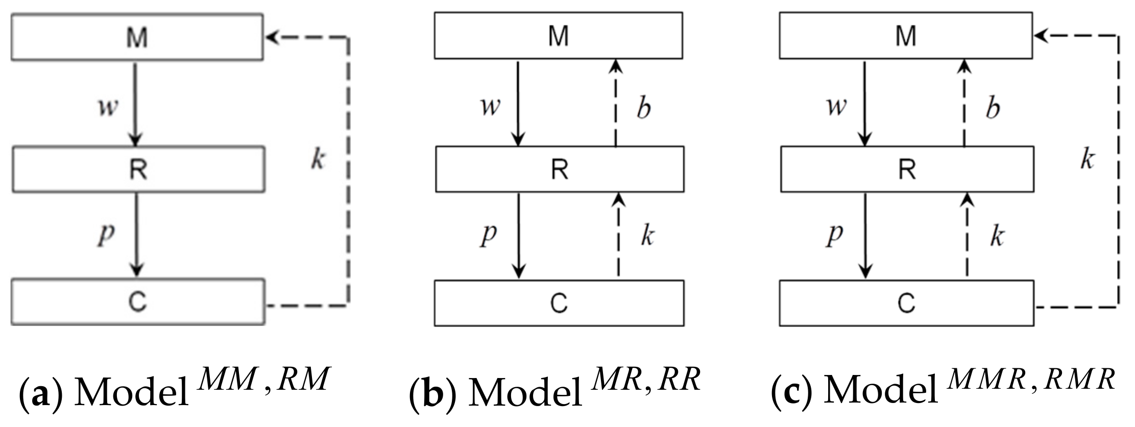
4. Model Development

4.1. Manufacturer Recycling Model

In this model, the manufacturer collects used products directly from the consumers and gives them a recycling subsidy for each returned product. The profit functions of the manufacturer and the retailer are respectively as follows:

$${\pi }_m(w,{\tau }_m)=(\alpha -p\beta )(w-c_m)-k(\alpha -p\beta ){\tau }_m+(\alpha -p\beta )\mathsf{\Delta }{\tau }_m-\frac{1}{2}h{\tau }_m^2$$

(1)

$${\pi }_r(p)=(p-w)(\alpha -p\beta )$$

(2)

4.1.1. Model $MM$: Manufacturer recycling Model Led by the Manufacturer

When the manufacturer acts as the Stackelberg leader, he first announces the wholesale price and recycling rate. Second, the retailer determines the retail price based on the manufacturer’s decision. Backward induction is used to solve the optimizations. The optimal solutions of Model $MM$ can be easily derived and given in Proposition 1.

Proposition 1. 

The Stackelberg equilibrium strategy of Model$MM$is:

$$\begin{array}{l}{w}^{MM}=\frac{\alpha (2h-\beta {(\mathsf{\Delta }-k)}^2)+2h\beta c_m}{\beta (4h-\beta {(\mathsf{\Delta }-k)}^2)}, {\tau }^{MM}={\tau }_m^{MM}=\frac{(\mathsf{\Delta }-k)(\alpha -\beta c_m)}{4h-\beta {(\mathsf{\Delta }-k)}^2}, p^{MM}=\frac{\alpha (3h-\beta {(\mathsf{\Delta }-k)}^2)+h\beta c_m}{\beta (4h-\beta {(\mathsf{\Delta }-k)}^2)},\\ Q^{MM}=\frac{h(\alpha -\beta c_m)}{4h-\beta {(\mathsf{\Delta }-k)}^2},{\pi }_m^{MM}=\frac{h{(\alpha -\beta c_m)}^2}{2\beta (4h-\beta {(\mathsf{\Delta }-k)}^2)}, {\pi }_r^{MM}=\frac{h^2{(\alpha -\beta c_m)}^2}{\beta {(4h-\beta {(\mathsf{\Delta }-k)}^2)}^2},\\ {\pi }^{MM}=\frac{h(6h-\beta {(k-\mathsf{\Delta })}^2){(\alpha -\beta c_m)}^2}{2\beta {(4h-\beta {(\mathsf{\Delta }-k)}^2)}^2}.\end{array}$$

Proof. 

See Appendix A.1. □

4.1.2. Model $RM$: Manufacturer Recycling Model Led by the Retailer

When the retailer is in the Stackelberg leadership position of the supply chain system, he first determines the retail price. Based on it, the manufacturer who acts as a follower estimates the wholesale price and recycling rate. Through backward induction, the equilibrium results of Model $RM$ can be found and depicted in Proposition 2.

Proposition 2. 

The Stackelberg equilibrium strategy of Model$RM$is:

$$\begin{array}{l}{w}^{RM}=\frac{2h\beta c_m+(h-\beta {(k-\mathsf{\Delta })}^2)(\alpha +\beta c_m)}{2\beta (2h-\beta {(\mathsf{\Delta }-k)}^2)},{\tau }^{RM}={\tau }_m^{RM}=\frac{(\mathsf{\Delta }-k)(\alpha -\beta c_m)}{4h-2\beta {(\mathsf{\Delta }-k)}^2},\\ p^{RM}=\frac{\alpha (3h-2\beta {(\mathsf{\Delta }-k)}^2)+h\beta c_m}{2\beta (2h-\beta {(\mathsf{\Delta }-k)}^2)},Q^{RM}=\frac{h(\alpha -\beta c_m)}{4h-2\beta {(\mathsf{\Delta }-k)}^2},{\pi }_m^{RM}=\frac{h{(\alpha -\beta c_m)}^2}{8\beta (2h-\beta {(\mathsf{\Delta }-k)}^2)},\\ {\pi }_r^{RM}=\frac{h{(\alpha -\beta c_m)}^2}{4\beta (2h-\beta {(\mathsf{\Delta }-k)}^2)},{\pi }^{RM}=\frac{3h{(\alpha -\beta c_m)}^2}{8\beta (2h-\beta {(\mathsf{\Delta }-k)}^2)}.\end{array}$$

Proof. 

See Appendix A.2. □

4.1.3. Comparison between Manufacturer Recycling Models under Different Channel Power Structures

Proposition 3.

${\pi }_m^{MM}>{\pi }_m^{RM}$, ${\pi }_r^{MM}<{\pi }_r^{RM}$, ${\pi }^{MM}<{\pi }^{RM}$

Proof. 

See Appendix A.3. □

Proposition 3 demonstrates that under the manufacturer recycling model, both the manufacturer and the retailer benefit more from the self-led supply chain. However, the system is more profitable under the retailer’s dominance. Since the recycling strategy of the retailer is consistent with that of the whole system, a giant retailer will create higher profit for the CLSC with manufacturer recycling.

4.2. Retailer Recycling Model

In this model, the retailer is not only responsible for product sales but also provide recycling service for the customers. The customers who send back the used products can receive a recycling subsidy given by the retailer. Then, the manufacturer buys back the returned products from the retailer for remanufacturing. The profit functions of the manufacturer and the retailer are respectively as follows:

$${\pi }_m(w)=(\alpha -p\beta )(w-c_m)+(\alpha -p\beta )\mathsf{\Delta }{\tau }_r-b(\alpha -p\beta ){\tau }_r$$

(3)

$${\pi }_r(p,{\tau }_r)=(p-w)(\alpha -p\beta )+(b-k)(\alpha -p\beta ){\tau }_r-\frac{1}{2}h{\tau }_r^2$$

(4)

4.2.1. Model $MR$: Retailer Recycling Model Led by the Manufacturer

When the manufacturer has sufficient channel power over the retailer, he first chooses the wholesale price. Second, the retailer determines the retail price and recycling rate in response to the manufacturer’s decision. Backward induction method is utilized to find the optimal solutions of Model $MR$ as shown in Proposition 4.

Proposition 4. 

The Stackelberg equilibrium strategy of Model$MR$is:

$$\begin{array}{l}{w}^{MR}=\frac{\alpha +\beta c_m}{2\beta },{\tau }^{MR}={\tau }_r^{MR}=\frac{(\mathsf{\Delta }-k)(\alpha -\beta c_m)}{4h-2\beta {(\mathsf{\Delta }-k)}^2},p^{MR}=\frac{\alpha (3h-2\beta {(\mathsf{\Delta }-k)}^2)+h\beta c_m}{2\beta (2h-\beta {(\mathsf{\Delta }-k)}^2)},\\ Q^{MR}=\frac{h(\alpha -\beta c_m)}{4h-2\beta {(\mathsf{\Delta }-k)}^2},{\pi }_m^{MR}=\frac{h{(\alpha -\beta c_m)}^2}{4\beta (2h-\beta {(\mathsf{\Delta }-k)}^2)},{\pi }_r^{MR}=\frac{h{(\alpha -\beta c_m)}^2}{8\beta (2h-\beta {(\mathsf{\Delta }-k)}^2)},\\ {\pi }^{MR}=\frac{3h{(\alpha -\beta c_m)}^2}{8\beta (2h-\beta {(\mathsf{\Delta }-k)}^2)}\end{array}$$

Proof. 

See Appendix B.1. □

4.2.2. Model $RR$: Retailer Recycling Model Led by the Retailer

When the retailer is the leading enterprise, he first estimates the retail price and recycling rate. Following the retailer’s decision, the manufacturer determines the wholesale price. Based on backward induction, the equilibrium results of Model $RR$ can be easily derived and given in Proposition 5.

Proposition 5. 

The Stackelberg equilibrium strategy of Model$RR$is:

$$\begin{array}{l}{w}^{RR}=\frac{\alpha (h+\beta (b-\mathsf{\Delta })(-k+\mathsf{\Delta }))+\beta (3h+(b-k)\beta (k-\mathsf{\Delta }))c_m}{\beta (4h-\beta {(k-\mathsf{\Delta })}^2)},{\tau }^{RR}={\tau }_r^{RR}=\frac{(k-\mathsf{\Delta })(-\alpha +\beta c_m)}{4h-\beta {(k-\mathsf{\Delta })}^2},\\ p^{RR}=\frac{\alpha (3h-\beta {(k-\mathsf{\Delta })}^2)+h\beta c_m}{\beta (4h-\beta {(k-\mathsf{\Delta })}^2)},Q^{RR}=\frac{h(\alpha -\beta c_m)}{4h-\beta {(\mathsf{\Delta }-k)}^2},{\pi }_m^{RR}=\frac{h^2{(\alpha -\beta c_m)}^2}{\beta {(4h-\beta {(k-\mathsf{\Delta })}^2)}^2},\\ {\pi }_r^{RR}=\frac{h{(\alpha -\beta c_m)}^2}{2\beta (4h-\beta {(k-\mathsf{\Delta })}^2)},{\pi }^{RR}=\frac{h(6h-\beta {(k-\mathsf{\Delta })}^2){(\alpha -\beta c_m)}^2}{2\beta {(4h-\beta {(k-\mathsf{\Delta })}^2)}^2}\end{array}$$

Proof. 

See Appendix B.2. □

4.2.3. Comparison between Retailer Recycling Models under Different Channel Power Structures

Proposition 6.

${\pi }_m^{MR}>{\pi }_m^{RR}$, ${\pi }_r^{MR}<{\pi }_r^{RR}$, ${\pi }^{MR}>{\pi }^{RR}$.

Proof. 

See Appendix B.3. □

Proposition 6 reveals that when the retailer is responsible for the product recycling independently, each member still prefers the supply chain led by himself. While from the view of the entire system, the manufacturer-led model is superior to the other one. Hence, a dominant manufacturer can make significant improvements to the profitability of the supply chain with retailer recycling.

4.3. Hybrid Recycling Model

The manufacturer and the retailer collect used products from the customers simultaneously, and then the retailer delivers these products to the manufacturer. Both of them pay to the customers for per unit returned product. The profit functions of the manufacturer and the retailer are respectively as follows:

$${\pi }_m=(\alpha -p\beta )(w-c_m)-k{\tau }_m(\alpha -p\beta )+\mathsf{\Delta }({\tau }_m+{\tau }_r)(\alpha -p\beta )-b{\tau }_r(\alpha -p\beta )-\frac{1}{2}h{\tau }_m^2$$

(5)

$${\pi }_r=(p-w)(\alpha -p\beta )+(b-k)(\alpha -p\beta ){\tau }_r-\frac{1}{2}h{\tau }_r^2$$

(6)

4.3.1. Model $MMR$: Hybrid Recycling Model Led by the Manufacturer

Consistent with the sequence of decision-making in Model $MR$, the manufacturer first announces the wholesale price and his recycling rate. Then the retailer determines the retail price and his own recycling rate based on the manufacturer’s decision. Backward induction is used to solve this game. The optimal solutions of Model $MMR$ can be acquired and depicted in Proposition 7.

Proposition 7. 

The Stackelberg equilibrium strategy of Model$MMR$is:

$$\begin{array}{l}{w}^{MMR}=\frac{\alpha (2h-2\beta {(\mathsf{\Delta }-k)}^2)+\beta (2h-\beta {(\mathsf{\Delta }-k)}^2)c_m}{\beta (4h-3\beta {(\mathsf{\Delta }-k)}^2)},{\tau }^{MMR}={\tau }_m{}^{MMR}+{\tau }_r{}^{MMR}=\frac{2(\mathsf{\Delta }-k)(\alpha -\beta c_m)}{4h-3\beta {(\mathsf{\Delta }-k)}^2},\\ p^{MMR}=\frac{\alpha (3h-3\beta {(\mathsf{\Delta }-k)}^2)+h\beta c_m}{\beta (4h-3\beta {(\mathsf{\Delta }-k)}^2)}, Q^{MMR}=\frac{h(\alpha -\beta c_m)}{4h-3\beta {(\mathsf{\Delta }-k)}^2}, {\pi }_m^{MMR}=\frac{h{(\alpha -\beta c_m)}^2}{2\beta (4h-3\beta {(\mathsf{\Delta }-k)}^2)},\\ {\pi }_r^{MMR}=\frac{h(2h-{(\mathsf{\Delta }-k)}^2\beta ){(\alpha -\beta c_m)}^2}{2\beta {(4h-3\beta {(\mathsf{\Delta }-k)}^2)}^2}, {\pi }^{MMR}=\frac{h(3h-2\beta {(\mathsf{\Delta }-k)}^2){(\alpha -\beta c_m)}^2}{\beta {(4h-3\beta {(\mathsf{\Delta }-k)}^2)}^2}\end{array}$$

Proof. 

See Appendix C.1. □

4.3.2. Model $RMR$: Hybrid Recycling Model Led by the Retailer

When the retailer acts as the channel leader, he first chooses the retail price and his recycling rate. Following the retailer’s decision, the manufacturer determines the wholesale price and his own recycling rate. By backward induction, the equilibrium results of Model $RMR$ can be obtained and presented in Proposition 8.

Proposition 8. 

The Stackelberg equilibrium strategy of Model$RMR$is:

$$\begin{array}{l}{w}^{RMR}=\frac{\alpha (h-\beta (b+k-2\mathsf{\Delta })(k-\mathsf{\Delta }))+\beta (3h+\beta (k-\mathsf{\Delta })(b-2k+\mathsf{\Delta }))c_m}{\beta (4h-3\beta {(k-\mathsf{\Delta })}^2)},\\ {\tau }^{RMR}={\tau }_m{}^{RMR}+{\tau }_r{}^{RMR}=\frac{2(\mathsf{\Delta }-k)(\alpha -\beta c_m)}{4h-3\beta {(k-\mathsf{\Delta })}^2},p^{RMR}=\frac{3\alpha (h-\beta {(\mathsf{\Delta }-k)}^2)+h\beta c_m}{\beta (4h-3\beta {(\mathsf{\Delta }-k)}^2)},\\ Q^{RMR}=\frac{h(\alpha -\beta c_m)}{4h-3\beta {(k-\mathsf{\Delta })}^2},{\pi }_m^{RMR}=\frac{h(2h-\beta {(\mathsf{\Delta }-k)}^2){(\alpha -\beta c_m)}^2}{2\beta {(4h-3\beta {(\mathsf{\Delta }-k)}^2)}^2},{\pi }_r^{RMR}=\frac{h{(\alpha -\beta c_m)}^2}{2\beta (4h-3\beta {(\mathsf{\Delta }-k)}^2)},\\ {\pi }^{RMR}=\frac{h(3h-2\beta {(k-\mathsf{\Delta })}^2){(\alpha -\beta c_m)}^2}{\beta {(4h-3\beta {(k-\mathsf{\Delta })}^2)}^2}\end{array}$$

Proof. 

See Appendix C.2. □

4.3.3. Comparison between Hybrid Recycling Models under Different Channel Power Structures

Proposition 9.

${\pi }_m^{MMR}>{\pi }_m^{RMR}$, ${\pi }_r^{MMR}<{\pi }_r^{RMR}$, ${\pi }^{MMR}={\pi }^{RMR}$.

Proof. 

See Appendix C.3. □

Proposition 9 suggests that although both supply chain members are partial to the self-led hybrid recycling models, there is no difference between the two systems in terms of the total profits. According to the equilibrium solutions in Propositions 7 and 8, we have ${\tau }^{MMR}=t^{RMR}$ and $Q^{MMR}=Q^{RMR}$. Therefore, different channel leaderships have no effect on the system efficiency of the CLSC with hybrid recycling of manufacturer and retailer.

5. Comparative Analysis

By comparing the equilibrium solutions of the above models, some significant findings can be obtained as follows.

5.1. Comparison of Market Demands and Recycling Rates among Different Models

Proposition 10.

${\tau }^{MMR}={\tau }^{RMR}>{\tau }^{MR}={\tau }^{RM}>{\tau }^{MM}={\tau }^{RR}$, $Q^{MMR}=Q^{RMR}>Q^{MR}=Q^{RM}>Q^{MM}=Q^{RR}$.

Proof. 

See Appendix D.1. □

Proposition 10 shows that the hybrid recycling models not only have the highest recycling rate of the whole system but also achieve the highest market demand. Contrarily, Model $MM$ and Model $RR$, the CLSCs in which the channel leader collects used products, perform poorly in the total recycling rate and the demand for the product in the market. The follower recycling models such as Model $MR$ and Model $RM$ are ranked in the middle. Therefore, homologous sequences of total recycling quantities under different models can be found. Thus, we can conclude that whether in the manufacturer-led system or in the retailer-led system, the hybrid recycling model is the optimal approach to collect used products, and it can realize high efficiency of resource utilization and recycling.

5.2. Comparison of Models Led by the Manufacturer

Proposition 11.

${\pi }_m^{MMR}>{\pi }_m^{MR}>{\pi }_m^{MM}$, ${\pi }_r^{MMR}>{\pi }_r^{MR}>{\pi }_r^{MM}$.

Proof. 

See Appendix D.2. □

Proposition 11 proves that in the manufacturer-led CLSC with hybrid recycling channels, the profits of both members are always higher than the profits received in the other two single recycling models. Furthermore, the optimal recycling strategy of the retailer is consistent with that of the dominant manufacturer. Therefore, the manufacturer has a strong incentive to collect used products with the retailer, and long-term stability of the supply chain system will be maintained.

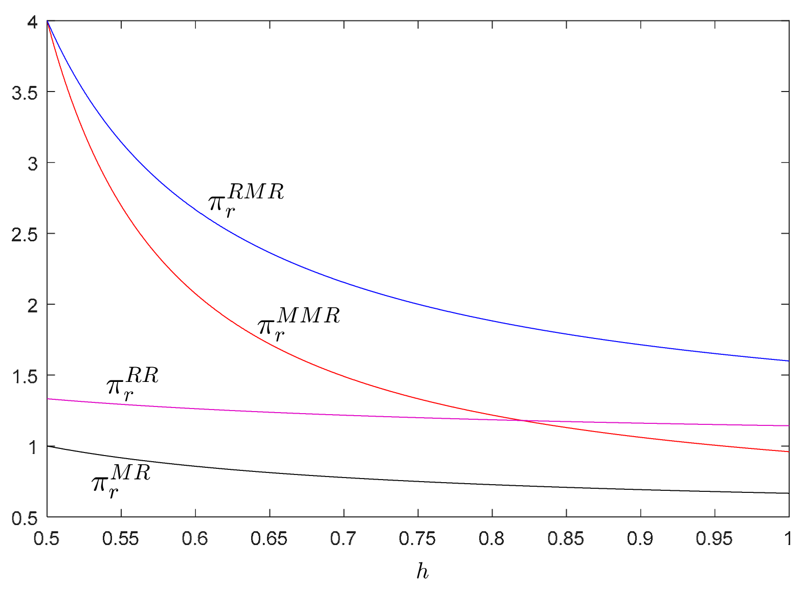
5.3. Comparison of Models Led by the Retailer

Proposition 12.

${\pi }_m^{RMR}>{\pi }_m^{RM}>{\pi }_m^{RR}$, ${\pi }_r^{RMR}>{\pi }_r^{RM}>{\pi }_r^{RR}$.

Proof. 

See Appendix D.3. □

The analysis of the retailer-led CLSCs is similar to the above. Proposition 12 indicates that the hybrid recycling model is always preferable for both channel members, and the corresponding system can remain stable. While when there are only retailer recycling use products in the supply chain, the profits of the supply chain members would fall to their lowest. In this case, the retailer won’t collect used products independently.

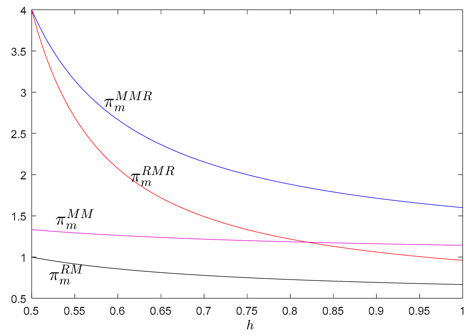
5.4. Comparison of Models with Manufacturer’s Participation in Recycling

Proposition 13.

(1)

If$\beta {(\mathsf{\Delta }-k)}^2<h<\frac{9+\sqrt{17}}{8}\beta {(\mathsf{\Delta }-k)}^2$, then${\pi }_m^{MMR}>{\pi }_m^{RMR}>{\pi }_m^{MM}>{\pi }_m^{RM}$;

(2)

if$h>\frac{9+\sqrt{17}}{8}\beta {(\mathsf{\Delta }-k)}^2$, then${\pi }_m^{MMR}>{\pi }_m^{MM}>{\pi }_m^{RMR}>{\pi }_m^{RM}$.

Proof. 

See Appendix D.4. □

Proposition 13 suggests that when the manufacturer participates in the recycling activity, Model $MMR$ is his optimal strategy, while Model $RM$ is his least preferred option. Since there is only one leading enterprise in the CLSC system, if the manufacturer is the channel leader, he should adopt the hybrid recycling mode; if the manufacturer is the following enterprise, he also should cooperate with the dominator, the retailer who implements the strategy of hybrid recycling. Therefore, as long as the manufacturer participates in the recycling of waste products, the hybrid recycling of supply chain members is always the optimal choice for him.

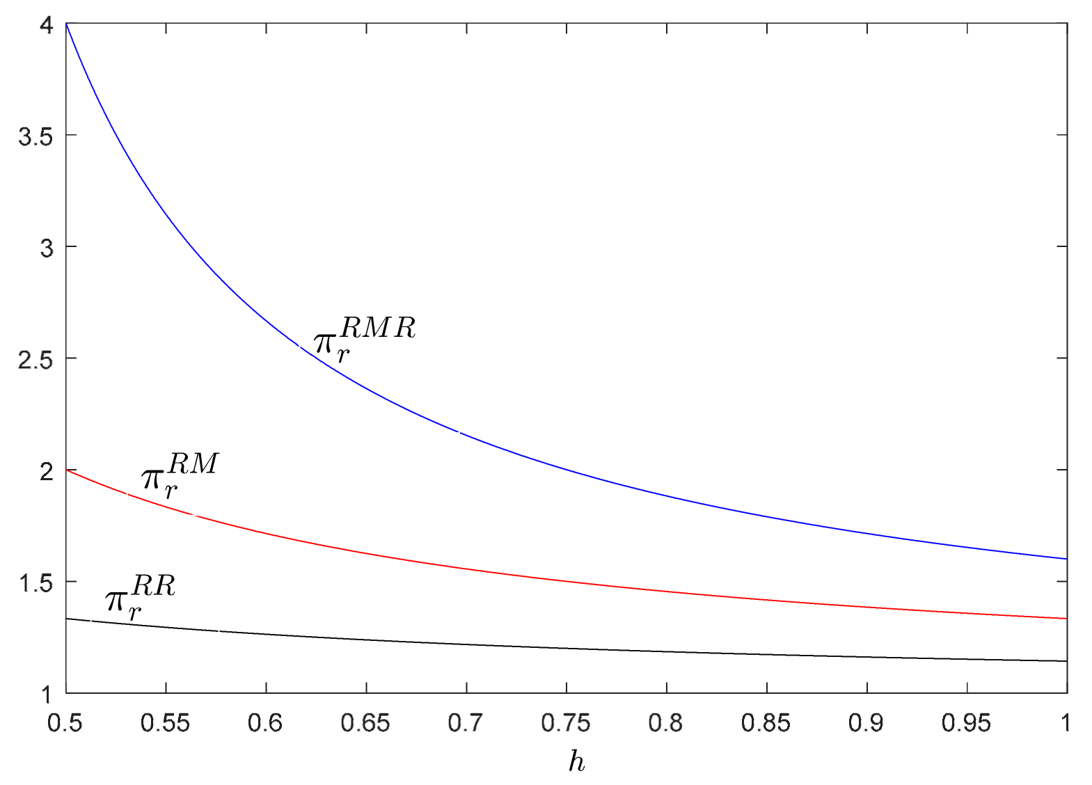
5.5. Comparison of Models with Retailer’s Participation in Recycling

Proposition 14.

(1)

If$\beta {(\mathsf{\Delta }-k)}^2<h<\frac{9+\sqrt{17}}{8}\beta {(\mathsf{\Delta }-k)}^2$, then${\pi }_r^{RMR}>{\pi }_r^{MMR}>{\pi }_r^{RR}>{\pi }_r^{MR}$;

(2)

if$h>\frac{9+\sqrt{17}}{8}\beta {(\mathsf{\Delta }-k)}^2$, then${\pi }_r^{RMR}>{\pi }_r^{RR}>{\pi }_r^{MMR}>{\pi }_r^{MR}$

Proof. 

See Appendix D.5. □

Proposition 14 proves that among the CLSCs with retailer’s recycling involvement, Model $RMR$ is his optimal choice, while Model $MR$ performs poorly in terms of the retailer’s profit. Like the above analysis of Proposition 13, whether the retailer is in the Stackelberg leadership position or not, he will benefit more from the hybrid recycling mode, when compared with the model with only the retailer recycling used products. Hence, the retailer will always choose the cooperative strategy to engage in the product recycling.

6. Optimal Strategies of Leading Enterprise and Following Enterprise

To obtain more general results, we compare the equilibrium profits of the manufacturer, the retailer and the supply chain system in the following.

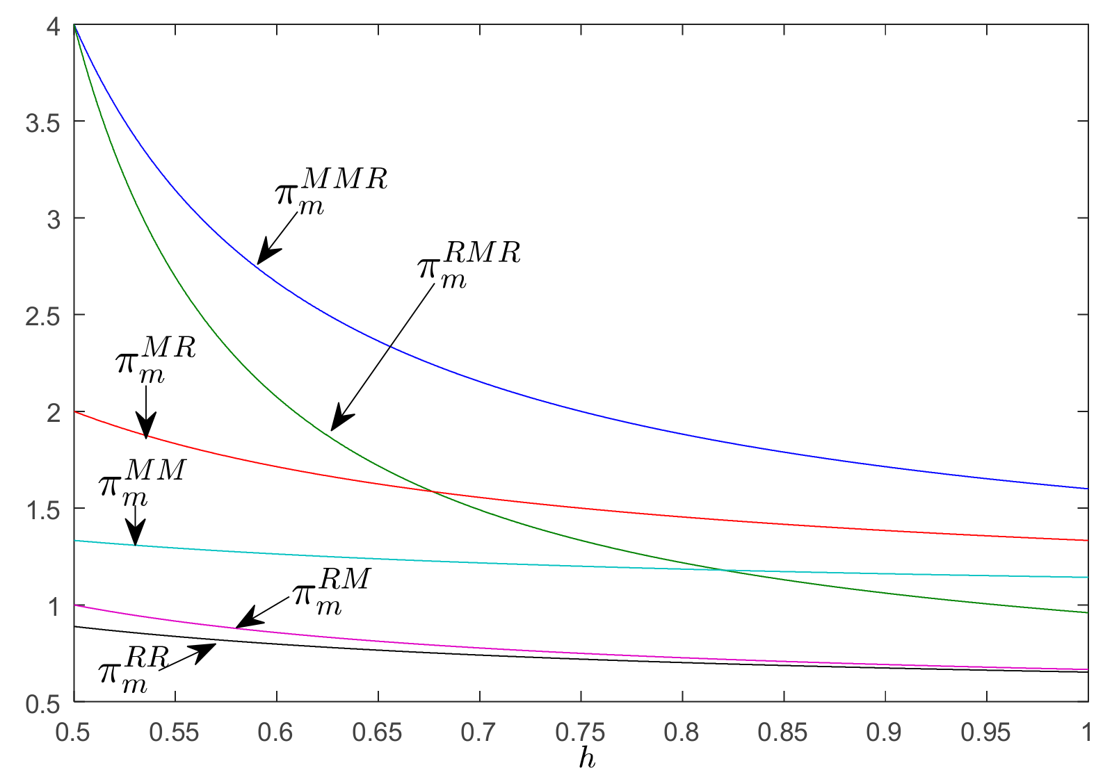
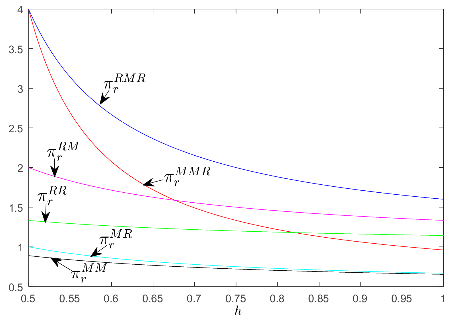
6.1. Comparison of Profits of Supply Chain Members among Different Models

Proposition 15.

(1)

If$\beta {(\mathsf{\Delta }-k)}^2<h<\frac{4+\sqrt{2}}{4}\beta {(\mathsf{\Delta }-k)}^2$, then${\pi }_m^{MMR}>{\pi }_m^{RMR}>{\pi }_m^{MR}>{\pi }_m^{MM}>{\pi }_m^{RM}>{\pi }_m^{RR}$and${\pi }_r^{RMR}>{\pi }_r^{MMR}>{\pi }_r^{RM}>{\pi }_r^{RR}>{\pi }_r^{MR}>{\pi }_r^{MM}$;

(2)

if$\frac{4+\sqrt{2}}{4}\beta {(\mathsf{\Delta }-k)}^2<h<\frac{9+\sqrt{17}}{8}\beta {(\mathsf{\Delta }-k)}^2$, then${\pi }_m^{MMR}>{\pi }_m^{MR}>{\pi }_m^{RMR}>{\pi }_m^{MM}>{\pi }_m^{RM}>{\pi }_m^{RR}$and${\pi }_r^{RMR}>{\pi }_r^{RM}>{\pi }_r^{MMR}>{\pi }_r^{RR}>{\pi }_r^{MR}>{\pi }_r^{MM}$;

(3)

if$h>\frac{9+\sqrt{17}}{8}\beta {(\mathsf{\Delta }-k)}^2$, then${\pi }_m^{MMR}>{\pi }_m^{MR}>{\pi }_m^{MM}>{\pi }_m^{RMR}>{\pi }_m^{RM}>{\pi }_m^{RR}$and${\pi }_r^{RMR}>{\pi }_r^{RM}>{\pi }_r^{RR}>{\pi }_r^{MMR}>{\pi }_r^{MR}>{\pi }_r^{MM}$

Proof. 

See Appendix D.6. □

Proposition 15 demonstrates that the optimal choice of the manufacturer is Model $MMR$, the self-led hybrid recycling model. From the manufacturer’s perspective, Model $RM$ and Model $RR$ are ranked in 5th and 6th place respectively among all six recycling models, which are always his worst selections. When the sensitivity coefficient to the unit recycling cost is relatively low ($\beta {(\mathsf{\Delta }-k)}^2<h<\frac{4+\sqrt{2}}{4}\beta {(\mathsf{\Delta }-k)}^2$), Model $RMR$ is the second best choice for the manufacturer, and Model $MR$ and Model $MM$ are ranked at 3rd and 4th respectively. However, we also find that with the increase of the sensitivity coefficient, the advantage of Model $RMR$ for the manufacturer weakens continually, while the rankings of Model $MM$ and Model $MR$ are gradually improving. That is, as the sensitivity coefficient to the unit recycling cost increases, the recycling models tend to be more profitable for the leading enterprise. The analysis of the retailer’s strategy is similar to the above so we will not repeat it here.

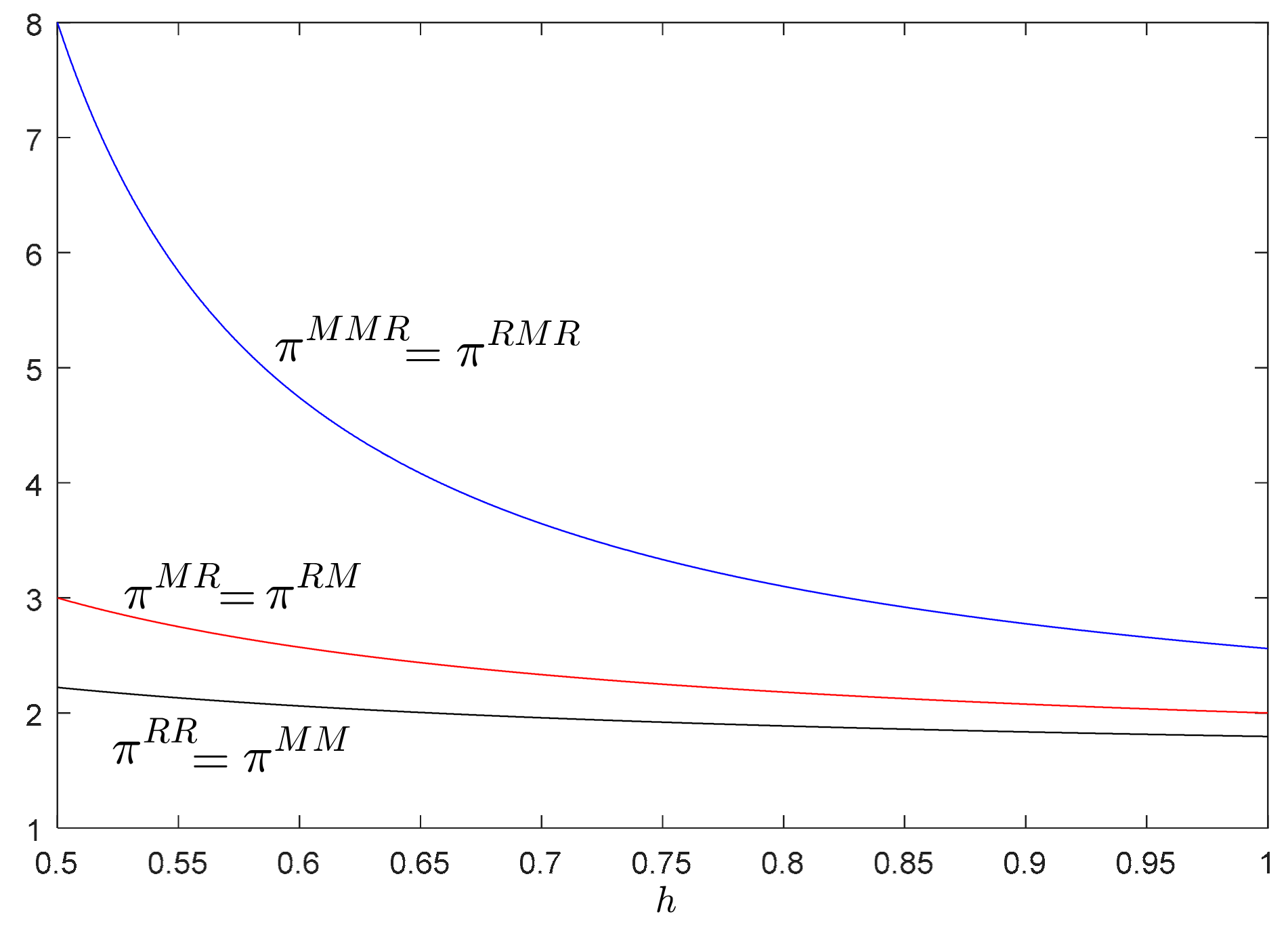
6.2. Comparison of Profits of Supply Chain System among Different Models

Proposition 16.

${\pi }^{MMR}={\pi }^{RMR}>{\pi }^{MR}={\pi }^{RM}>{\pi }^{RR}={\pi }^{MM}$.

Proof. 

See Appendix D.7. □

Proposition 16 implies that the hybrid recycling models perform better than the single recycling models, whereas the supply chains in which only the channel leader collects used products are the least preferred options. Combining Proposition 10, we can conclude that from a practical viewpoint, the hybrid recycling mode is superior in terms of resource utilization and environmental protection.

Propositions 15–16 analyze the optimal decisions of the channel members and the overall system under different recycling models, respectively. As the supply chain members operate independently to pursue optimization of individual benefits, the recycling model chosen by the leading enterprise is not necessarily the optimal strategy for the follower. Nevertheless, in the real market, the following enterprise has to make business decisions based on that of the channel leader. To derive the optimal strategies of leading enterprise and following enterprise, we rank the results as shown in

Table 2. Ranking list.

Ranking of Profits		1	2	3	4	5	6
$\beta {(\mathsf{\Delta }-k)}^2<h<\frac{4+\sqrt{2}}{4}\beta {(\mathsf{\Delta }-k)}^2$	${\pi }_m$	MMR	RMR	MR	MM	RM	RR
	${\pi }_r$	RMR	MMR	RM	RR	MR	MM
$\frac{4+\sqrt{2}}{4}\beta {(\mathsf{\Delta }-k)}^2<h<\frac{9+\sqrt{17}}{8}\beta {(\mathsf{\Delta }-k)}^2$	${\pi }_m$	MMR	MR	RMR	MM	RM	RR
	${\pi }_r$	RMR	RM	MMR	RR	MR	MM
$h>\frac{9+\sqrt{17}}{8}\beta {(\mathsf{\Delta }-k)}^2$	${\pi }_m$	MMR	MR	MM	RMR	RM	RR
	${\pi }_r$	RMR	RM	RR	MMR	MR	MM
$\pi$: MMR = RMR > MR = RM > MM = RR

.

As indicated in Table 2, the leading enterprise is always partial to the self-led hybrid recycling model, which is also the optimal choice for the follower among all three recycling models led by this channel leader. And from the view of the whole system, the hybrid recycling mode can realize highly efficient utilization and recycling of resources. Furthermore, the advantage of self-led recycling models is being strengthened with the increase of the sensitivity coefficient to the unit recycling cost. Table 2 also illustrates that when there is only one collector in the CLSC, the leading enterprise always prefers the follower recycling model, while it is the third best choice for the following enterprise. For each supply chain member, the worst choices are the single recycling models led by the other one, and the efficiency of these systems is also ranked at the bottom of the list. Thus, the leading enterprise has a strong incentive to collect used products with the follower, and the hybrid recycling strategy now has become the development direction in recycling industry.

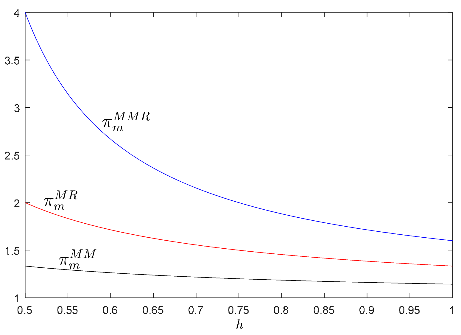
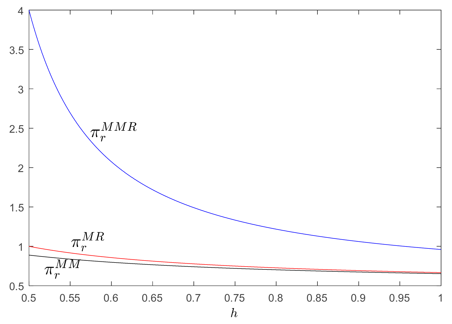
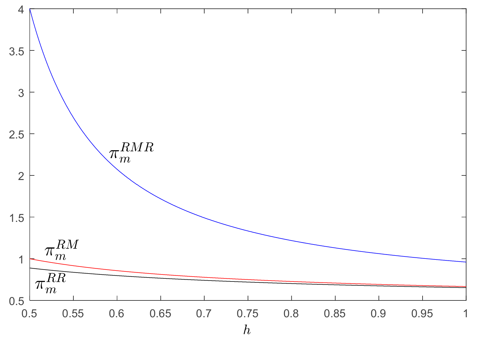
7. Numerical Examples

Considering model rationality, the values of the key parameters are assumed as follows: $\alpha =4$, $\beta =0.5$, $c_m=4$, $c_r=2$, $k=1$. Then we have $\beta {(\mathsf{\Delta }-k)}^2=0.5$, $\frac{4+\sqrt{2}}{4}\beta {(\mathsf{\Delta }-k)}^2=0.68$ and $\frac{9+\sqrt{17}}{8}\beta {(\mathsf{\Delta }-k)}^2=0.82$. In particular, according to the conditions set for the ranges of $h$, the value of $h$ should satisfy $h>0.5$. Under the present parameter settings, profits of supply chain members and entire system under different recycling models can be derived as presented in the following.

As clearly shown in Figure 2 and Figure 3, when the manufacturer acts as the channel leader, both members’ profits in the hybrid recycling model are the greatest; however, the single recycling of the retailer and the manufacturer are respectively the second and the least preferred option for each member, which is consistent with our findings in Proposition 11.

Similarly, Figure 4 and Figure 5 indicate that in the retailer-led CLSC, the manufacturer and the retailer can gain more benefits from the hybrid recycling strategy, while both members’ profits in the manufacturer recycling and retailer recycling model are ranked at 2nd and 3rd respectively, which further proves Proposition 12.

Figure 6 illustrates that when the manufacturer participates in the recycling activity, the self-led hybrid recycling model is his optimal choice, whereas the retailer-led manufacturer recycling model is extremely inefficient. Moreover, it demonstrates that the relation between manufacturer’s profits in the retailer-led hybrid recycling model, and the manufacturer-led manufacturer recycling model depends on the sensitivity coefficient to the unit recycling cost. When the sensitivity coefficient is relatively low ($0.5<h<0.68$), the manufacturer prefers the retailer-led hybrid recycling model; otherwise, the self-led manufacturer recycling model is superior. The explanation of Figure 7, which describes the retailer’s strategy when he participates in the product recycling is similar to the above, and these confirm our analytical observations from Propositions 13 and 14.

From Figure 8, we can find that when the sensitivity coefficient to the unit recycling cost is relatively low ($0.5<h<0.68$), the manufacturer’s profits follow the sequence ${\pi }_m^{MMR}>{\pi }_m^{RMR}>{\pi }_m^{MR}>{\pi }_m^{MM}>{\pi }_m^{RM}>{\pi }_m^{RR}$. As the sensitivity coefficient increases, the advantage of Model $RMR$ will diminish, and Model $MR$ and Model $MM$ will surpass it gradually. Similar to the analysis of the manufacturer’s profit, Figure 9 shows that for a lower sensitivity coefficient to the unit recycling cost ($0.5<h<0.68$), the retailer’s profits under different models are ranked as ${\pi }_r^{RMR}>{\pi }_r^{MMR}>{\pi }_r^{RM}>{\pi }_r^{RR}>{\pi }_r^{MR}>{\pi }_r^{MM}$. With the increase of the sensitivity coefficient, the retailer enjoys a higher profit in Model $RM$ and Model $RR$ which outperform Model $MMR$. It verifies that compared with the following enterprise, the channel leader benefit more from a higher sensitivity coefficient to the unit recycling cost. Hence, the results are exactly what we analytically find in Proposition 15.

Figure 10 shows that no matter who is the leading enterprise, the hybrid recycling models are more profitable than the single recycling models, while the CLSCs in which the channel leader collects used products independently are the least efficient systems. This matches with our findings in Proposition 16. From both the individual as well as the entire system point of view, the manufacturer and retailer hybrid recycling model is the optimal approach of product recycling, which can not only realize the profit maximization but also implement resource recycling and environmental protection. Therefore, in order to obtain a win-win situation in the market, both enterprises adopt cooperative strategy to engage in the recycling of waste products. In addition, to avoid potential conflicts between leading and following enterprises for efficient management of product recycling and remanufacturing, the government should lead the cooperation among the supply chain members.

8. Conclusions and Future Research Directions

This study develops three recycling models, namely manufacturer recycling, retailer recycling and hybrid recycling in a two-echelon CLSC consisting of a manufacturer and a retailer. To investigate the effect of different channel power structures on the optimal choices and profits of supply chain members, each model is discussed in manufacturer-led and retailer-led scenarios respectively. The equilibrium pricing, production and recycling decisions are determined analytically. From the comparative analysis and numerical study, we obtain some significant findings summarized as follows.

(1)

The hybrid recycling of manufacturer and retailer is always advantageous for the system recycling rate and market demand, while the supply chain in which the leading enterprise collects used products has the worst results in terms of total recycling rate and demand for the product in the market.

(2)

A dominant manufacturer (retailer) can provide higher profitability and greater stability to the supply chain system with retailer (manufacturer) recycling, whereas different channel leaderships have no effect on the system efficiency and stability of the CLSC with hybrid recycling channels.

(3)

In the manufacturer-led (retailer-led) CLSC, the optimal recycling strategy of both supply chain members is the hybrid recycling mode. However, their sub-optimal choice is the retailer (manufacturer) recycling model. The system with only one product collector performs poorly in system recycling rate and members’ profits.

(4)

Each supply chain member can be more profitable under the self-led hybrid recycling model which is also the optimal choice for the following enterprise, while the manufacturer (retailer) recycling model oriented by the manufacturer (retailer) is the least preferred strategy of the retailer (manufacturer).

(5)

For each supply chain member, as long as he participates in the product recycling, the hybrid recycling of both enterprises is the most effective strategy for him. Moreover, the advantage of self-led recycling models is being strengthened with the increase of the sensitivity coefficient to the unit recycling cost.

The insights derived from this study have several implications for both enterprises and government. First, under the same recycling modes, both manufacturer and retailer always benefit from their leadership. Thus, all supply chain members always want to act as a leader. However, the leadership cannot always guarantee that all the channel members would obtain more profits. Second, the efficiency of the entire supply chain remains the same under the same recycling modes with different power structures, while the hybrid collection of member enterprises ensures the whole supply chain system getting a better performance. Moreover, our research suggests that the hybrid recycling of supply chain members is the optimal approach to product recycling, which cannot only realize profit maximization but also implement resource recycling and environmental protection. Therefore, to avoid the worst consequences of single recycling mode, business managers should strengthen the cooperative awareness and jointly participate in the recycling of waste products to achieve a win-win situation in the market. Third, to alleviate channel conflict and promote the overall performance of the supply chain system, the government should exert its function of macro-supervisor: guide the channel members to form a strategic alliance with each other for efficient management of product recycling and remanufacturing.

Although our study offered several innovations, there were still a few deficiencies and limitations that should be ameliorated in future research. For instance, this study only considers manufacturer or retailer as the collector, while some manufacturers outsource product recycling to the retailer or the third-party in the real business environment. Therefore, further research can consider the hybrid recycling of retailer and third-party, or even take the recycling competition between the dual recycling channels into consideration. Furthermore, our models are developed based on a linear demand function. In view of the fact that some randomness may occur in demand due to different uncertainties, future research can also extend the model under the environment of stochastic demand instead of deterministic demand. Other possible extensions to this study include consideration of asymmetric information, consumer preferences and differential pricing strategies between new and remanufactured products.

References

1. Islam, M.T.; Abdullah, A.; Shahir, S.; Kalam, M.; Masjuki, H.; Shumon, R.; Rashid, M.H. A public survey on knowledge, awareness, attitude and willingness to pay for WEEE management: Case study in Bangladesh. J. Clean. Prod. 2016, 137, 728–740. [Google Scholar] [CrossRef]
2. Dai, D.; Si, F.; Wang, J. Stability and complexity analysis of a dual-channel closed-loop supply chain with delayed decision under government intervention. Entropy 2017, 19, 577. [Google Scholar] [CrossRef]
3. Baldé, C.P.; Forti, V.; Gray, V.; Kuehr, R.; Stegmann, P. The Global E-Waste Monitor 2017: Quantities, Flows and Resources; United Nations University (UNU): Bonn, Germany; International Telecommunication Union (ITU): Geneva, Switzerland; International Solid Waste Association (ISWA): Vienna, Austria, 2017. [Google Scholar]
4. Qu, Y.; Zhu, Q.; Sarkis, J.; Geng, Y.; Zhong, Y. A review of developing an e-wastes collection system in Dalian, China. J. Clean. Prod. 2013, 52, 176–184. [Google Scholar] [CrossRef]
5. Williams, E.; Kahhat, R.; Allenby, B.; Kavazanjian, E.; Kim, J.; Xu, M. Environmental, social, and economic implications of global reuse and recycling of personal computers. Environ. Sci. Technol. 2008, 42, 6446–6454. [Google Scholar] [CrossRef] [PubMed]
6. Wang, W.; Ding, J.; Sun, H. Reward-penalty mechanism for a two-period closed-loop supply chain. J. Clean. Prod. 2018, 203, 898–917. [Google Scholar] [CrossRef]
7. Wang, W.; Zhang, Y.; Zhang, K.; Bai, T.; Shang, J. Reward-penalty mechanism for closed-loop supply chains under responsibility-sharing and different power structures. Int. J. Prod. Econ. 2015, 170, 178–190. [Google Scholar] [CrossRef]
8. Wienold, J.; Recknagel, S.; Scharf, H.; Hoppe, M.; Michaelis, M. Elemental analysis of printed circuit boards considering the ROHS regulations. Waste Manag. 2011, 31, 530–535. [Google Scholar] [CrossRef]
9. Gutiérrez, E.; Adenso-Díaz, B.; Lozano, S.; González-Torre, P. A competing risks approach for time estimation of household WEEE disposal. Waste Manag. 2010, 30, 1643–1652. [Google Scholar] [CrossRef]
10. Kiddee, P.; Naidu, R.; Wong, M.H. Electronic waste management approaches: An overview. Waste Manag. 2013, 33, 1237–1250. [Google Scholar] [CrossRef]
11. Wäger, P.A.; Hischier, R.; Eugster, M. Environmental impacts of the Swiss collection and recovery systems for Waste Electrical and Electronic Equipment (WEEE): A follow-up. Sci. Total Environ. 2011, 409, 1746–1756. [Google Scholar] [CrossRef]
12. Menikpura, S.N.M.; Santo, A.; Hotta, Y. Assessing the climate co-benefits from Waste Electrical and Electronic Equipment (WEEE) recycling in Japan. J. Clean. Prod. 2014, 74, 183–190. [Google Scholar] [CrossRef]
13. Zhang, S.; Ding, Y.; Liu, B.; Pan, D.; Chang, C.; Volinsky, A. Challenges in legislation, recycling system and technical system of waste electrical and electronic equipment in China. Waste Manag. 2015, 45, 361–373. [Google Scholar] [CrossRef] [PubMed]
14. Lee, C.; Chang, S.; Wang, K.; Wen, L. Management of scrap computer recycling in Taiwan. J. Hazard. Mater. 2000, 73, 209–220. [Google Scholar] [CrossRef]
15. Savaskan, R.C.; Bhattacharya, S.; van Wassenhove, L.N. Closed-loop supply chain models with product remanufacturing. Manag. Sci. 2004, 50, 239–252. [Google Scholar] [CrossRef]
16. Liu, L.; Wang, Z.; Xu, L.; Hong, X.; Govindan, K. Collection effort and reverse channel choices in a closed-loop supply chain. J. Clean. Prod. 2017, 144, 492–500. [Google Scholar] [CrossRef]
17. EL korchi, A.; Millet, D. Designing a sustainable reverse logistics channel: The 18 generic structures framework. J. Clean. Prod. 2011, 19, 588–597. [Google Scholar] [CrossRef]
18. Yi, P.; Huang, M.; Guo, L.; Shi, T. Dual recycling channel decision in retailer oriented closed-loop supply chain for construction machinery remanufacturing. J. Clean. Prod. 2016, 137, 1393–1405. [Google Scholar] [CrossRef]
19. Lai, K.; Tang, A.K.Y. Green retailing: Factors for success. Calif. Manag. Rev. 2010, 52, 6–31. [Google Scholar] [CrossRef]
20. Styles, D.; Schoenberger, H.; Galvez-Martos, J.L. Environmental improvement of product supply chains: A review of European retailers’ performance. Resour. Conserv. Recyl. 2012, 65, 57–78. [Google Scholar] [CrossRef]
21. Chiu, C.H.; Choi, T.M.; Li, X.; Yiu, C.K.F. Coordinating supply chains with a general price-dependent demand function: Impacts of channel leadership and information asymmetry. IEEE Trans. Eng. Manag. 2016, 63, 390–403. [Google Scholar] [CrossRef]
22. Tong, W.; Mu, D.; Zhao, F.; Mendis, G.P.; Sutherland, J.W. The impact of cap-and-trade mechanism and consumers’ environmental preferences on a retailer-led supply Chain. Resour. Conserv. Recyl. 2019, 142, 88–100. [Google Scholar] [CrossRef]
23. Savaskan, R.C.; van Wassenhove, L.N. Reverse channel design: The case of competing retailers. Manag. Sci. 2006, 52, 1–14. [Google Scholar] [CrossRef]
24. Yao, W.; Chen, M. Comparison among closed-loop supply chain models. Commer. Resour. 2007, 1, 51–53. [Google Scholar]
25. Webster, S.; Mitra, S. Competitive strategy in remanufacturing and the impact of take-back laws. J. Oper. Manag. 2007, 25, 1123–1140. [Google Scholar] [CrossRef]
26. Karakayali, I.; Emir-Farinas, H.; Akcali, E. Pricing and recovery planning for remanufacturing operations with multiple used products and multiple reusable components. Comput. Ind. Eng. 2010, 59, 55–63. [Google Scholar] [CrossRef]
27. Atasu, A.; Sarvary, M.; van Wassenhove, L.N. Remanufacturing as a marketing strategy. Manag. Sci. 2008, 54, 1731–1746. [Google Scholar] [CrossRef]
28. Ferguson, M.E.; Souza, G.C. Closed-Loop Supply Chains—New Developments to Improve the Sustainability of Business Practices; Taylor & Francis Group: New York, NY, USA, 2010. [Google Scholar]
29. Zou, Z.B.; Wang, J.J.; Deng, G.S.; Chen, H. Third-party remanufacturing mode selection: Outsourcing or authorization? Transp. Res. Part E Logist. Transp. Rev. 2016, 87, 1–19. [Google Scholar] [CrossRef]
30. Hong, I.H.; Yeh, J.S. Modeling closed-loop supply chains in the electronics industry: A retailer collection application. Transp. Res. Part E Logist. Transp. Rev. 2012, 48, 817–829. [Google Scholar] [CrossRef]
31. Atasu, A.; van Wassenhove, L.N. An operations perspective on product take-back legislation for e-waste: Theory, practice, and research needs. Prod. Oper. Manag. 2012, 21, 407–422. [Google Scholar] [CrossRef]
32. Atasu, A.; Toktay, L.B.; van Wassenhove, L.N. How collection cost structure drives a manufacturer’s reverse channel choice. Prod. Oper. Manag. 2013, 22, 1089–1102. [Google Scholar] [CrossRef]
33. Wei, J.; Zhao, J. Reverse channel decisions for a fuzzy closed-loop supply chain. Appl. Math. Model. 2013, 37, 1502–1513. [Google Scholar] [CrossRef]
34. Chuang, C.H.; Wang, C.X.; Zhao, Y.B. Closed-loop supply chain models for a high-tech product under alternative reverse channel and collection cost structures. Int. J. Prod. Econ. 2014, 156, 108–123. [Google Scholar] [CrossRef]
35. de Giovanni, P.; Zaccour, G. A two-period game of a closed-loop supply chain. Eur. J. Oper. Res. 2014, 232, 22–40. [Google Scholar] [CrossRef]
36. Hong, X.; Xu, L.; Du, P.; Wang, W. Joint advertising, pricing and collection decisions in a closed-loop supply chain. Int. J. Prod. Econ. 2015, 167, 12–22. [Google Scholar] [CrossRef]
37. Maiti, T.; Giri, B.C. A closed loop supply chain under retail price and product quality dependent demand. J. Manuf. Syst. 2015, 37, 624–637. [Google Scholar] [CrossRef]
38. Genc, T.S.; de Giovanni, P. Trade-in and save: A two-period closed-loop supply chain game with price and technology dependent returns. Int. J. Prod. Econ. 2017, 183, 514–527. [Google Scholar] [CrossRef] [Green Version]
39. Xu, J.; Liu, N. Research on closed loop supply chain with reference price effect. J. Intell. Manuf. 2017, 28, 51–64. [Google Scholar] [CrossRef]
40. Govindan, K.; Soleimani, H.; Kannan, D. Reverse logistics and closed-loop supply chain: A comprehensive review to explore the future. Eur. J. Oper. Res. 2015, 240, 603–626. [Google Scholar] [CrossRef] [Green Version]
41. Govindan, K.; Soleimani, H. A review of reverse logistics and closed-loop supply chains: A journal of cleaner production focus. J. Clean. Prod. 2017, 142, 371–384. [Google Scholar] [CrossRef]
42. Modak, N.M.; Modak, N.; Panda, S.; Sana, S.S. Analyzing structure of two-echelon closed-loop supply chain for pricing, quality and recycling management. J. Clean. Prod. 2018, 171, 512–528. [Google Scholar] [CrossRef]
43. Huang, M.; Song, M.; Lee, L.H.; Ching, W.K. Analysis for strategy of closed-loop supply chain with dual recycling channel. Int. J. Prod. Econ. 2013, 144, 510–520. [Google Scholar] [CrossRef]
44. Ma, W.; Zhao, Z.; Ke, H. Dual-channel closed-loop supply chain with government consumption-subsidy. Eur. J. Oper. Res. 2013, 226, 221–227. [Google Scholar] [CrossRef]
45. Hong, X.P.; Wang, Z.J.; Wang, D.Z.; Zhang, H.G. Decision models of closed-loop supply chain with remanufacturing under hybrid dual-channel collection. Int. J. Adv. Manuf. Technol. 2013, 68, 1851–1865. [Google Scholar] [CrossRef]
46. Liu, H.; Lei, M.; Deng, H.; Leong, G.K.; Huang, T. A dual channel, quality-based price competition model for the WEEE recycling market with government subsidy. Omega 2016, 59, 290–302. [Google Scholar] [CrossRef]
47. de Giovanni, P.; Reddy, P.V.; Zaccour, G. Incentive strategies for an optimal recovery program in a closed-loop supply chain. Eur. J. Oper. Res. 2016, 249, 605–617. [Google Scholar] [CrossRef]
48. Feng, L.; Govindan, K.; Li, C. Strategic planning: Design and coordination for dual-recycling channel reverse supply chain considering consumer behavior. Eur. J. Oper. Res. 2017, 260, 601–612. [Google Scholar] [CrossRef]
49. Taleizadeh, A.A.; Moshtagh, M.S.; Moon, I. Pricing, product quality, and collection optimization in a decentralized closed-loop supply chain with different channel structures: Game theoretical approach. J. Clean. Prod. 2018, 189, 406–431. [Google Scholar] [CrossRef]
50. Mi, J.J.; Huang, Z.; Wang, K.; Tsai, S.B.; Li, G.; Wang, J. The presence of a powerful retailer on dynamic collecting closed-loop supply chain from a sustainable innovation perspective. Sustainability 2018, 10, 2115. [Google Scholar] [CrossRef] [Green Version]
51. Karakayali, I.; Emir-Farinas, H.; Akcali, E. An analysis of decentralized collection and processing of end-of-life products. J. Oper. Manag. 2007, 25, 1161–1183. [Google Scholar] [CrossRef]
52. Huang, Y.; Huang, G.Q. Price coordination in a three-level supply chain with different channel structures using game-theoretic approach. Int. J. Manag. Sci. Eng. Manag. 2010, 5, 83–94. [Google Scholar] [CrossRef]
53. Chen, K.; Zhuang, P. Disruption management for a dominant retailer with constant demand-stimulating service cost. Comput. Ind. Eng. 2011, 61, 936–946. [Google Scholar] [CrossRef]
54. Choi, T.M.; Li, Y.; Xu, L. Channel leadership, performance and coordination in closed loop supply chains. Int. J. Prod. Econ. 2013, 146, 371–380. [Google Scholar] [CrossRef]
55. Ma, P.; Wang, H.; Shang, J. Supply chain channel strategies with quality and marketing effort-dependent demand. Int. J. Prod. Econ. 2013, 144, 572–581. [Google Scholar] [CrossRef]
56. Zhao, J.; Wei, J.; Li, Y. Pricing decisions for substitutable products in a two-echelon supply chain with firms’ different channel powers. Int. J. Prod. Econ. 2014, 153, 243–252. [Google Scholar] [CrossRef]
57. Gao, J.; Han, H.; Hou, L.; Wang, H. Pricing and effort decisions in a closed-loop supply chain under different channel power structures. J. Clean. Prod. 2016, 112, 2043–2057. [Google Scholar] [CrossRef]
58. Taleizadeh, A.A.; Moshtagh, M.S.; Moon, I. Optimal decisions of price, quality, effort level and return policy in a three-level closed-loop supply chain based on different game theory approaches. Eur. J. Ind. Eng. 2017, 11, 486–525. [Google Scholar] [CrossRef] [Green Version]
59. Huang, H.; Ke, H. Pricing decision problem for substitutable products based on uncertainty theory. J. Intell. Manuf. 2017, 28, 503–514. [Google Scholar] [CrossRef]
60. Xu, Y.; Zhang, P. Decision-making in dual-channel green supply chain considering market structure. J. Serv. Sci. Manag. 2018, 11, 116–141. [Google Scholar] [CrossRef] [Green Version]
61. Zerang, E.S.; Taleizadeh, A.A.; Razmi, J. Analytical comparisons in a three-echelon closed-loop supply chain with price and marketing effort-dependent demand: Game theory approaches. Environ. Dev. Sustain. 2018, 20, 451–478. [Google Scholar] [CrossRef]
62. Jena, S.K.; Sarmah, S.P. Price competition and co-operation in a duopoly closed-loop supply chain. Int. J. Prod. Econ. 2014, 156, 346–360. [Google Scholar] [CrossRef]
63. Ma, Z.J.; Hu, S.; Dai, Y.; Ye, Y.S. Pay-as-you-throw versus recycling fund system in closed-loop supply chains with alliance recycling. Int. Trans. Oper. Res. 2018, 25, 1811–1829. [Google Scholar] [CrossRef]
64. Chen, J.M.; Chang, C.I. The co-operation strategy of a closed-loop supply chain with remanufacturing. Transp. Res. Part E Logist. Transp. Rev. 2012, 48, 387–400. [Google Scholar] [CrossRef]
Figure 1. Structure of CLSC models.
Sustainability 11 06413 g001
Figure 2. Manufacturer’s profits under manufacturer-led models.
Sustainability 11 06413 g002
Figure 3. Retailer’s profits under manufacturer-led models.
Sustainability 11 06413 g003
Figure 4. Manufacturer’s profits under retailer-led models.
Sustainability 11 06413 g004
Figure 5. Retailer’s profits under retailer-led models.
Sustainability 11 06413 g005
Figure 6. Manufacturer’s profits under models with manufacturer’s participation in recycling.
Sustainability 11 06413 g006
Figure 7. Retailer’s profits under models with retailer’s participation in recycling.
Sustainability 11 06413 g007
Figure 8. Manufacturer’s profits under different models.
Sustainability 11 06413 g008
Figure 9. Retailer’s profits under different models.
Sustainability 11 06413 g009
Figure 10. CLSC system’s profits under different models.
Sustainability 11 06413 g010