Life Cycle Assessment for Transportation Infrastructure Policy Evaluation and Procurement for State and Local Governments


 , , , ,
Abstract
:1. Introduction
- The net GHG reductions that result from implementing the strategies have often not been quantified;
- Few of the cases where GHG reductions have been quantified have used a system-wide perspective for their estimates;
- The time it will take to implement a strategy and begin achieving GHG reductions has not been considered;
- The process and difficulty of making the change have not been estimated, and;
- Most importantly, the costs, or in some cases savings, of implementing both initial and life cycle strategies have rarely been estimated in a way that prioritizes the most cost-effective strategies that would allow maximal emissions reductions with minimal costs.
- To evaluate possible changes that Caltrans can make in its operations to reduce GHG emissions
- To evaluate proposed actions for transportation in climate action plans that have been developed by cities and counties in California to reduce GHG emissions.
2. The Approach
3. Methodology
- Definition of the functional unit and system boundaries for the technology;
- Identification of available information;
- ○
- Technology of the strategy;
- ▪
- Initial implementation;
- ▪
- Life cycle, including maintenance, rehabilitation, replacement or end-of-life.
- ○
- Costs of the strategy;
- ○
- Constraints on implementation relevant to implementation by Caltrans.
- Creation of information;
- ○
- By analogous estimating from existing sources about similar technologies, different scales of research, development or implementation, or implementation in different contexts;
- ○
- By bottom-up estimation from existing sources about components of the technology.
- Calculations;
- ○
- Life cycle inventory and impacts;
- ○
- Initial costs;
- ○
- Life cycle costs.
- Assessment of data quality;
- Inclusion of the strategy on the supply curve.
- Define the change/technology; this question requires the proposer to specifically define the proposed change;
- Define the state of readiness of the change of technology using approach adapted from the NASA Technology Readiness Level system [38]; decision-makers are often not aware of the readiness of the proposed technology;
- TRL 1: basic principles observed;
- TRL 2: technology concept formulated;
- TRL 3 and 4: experimental proof of concept/ technology validated in lab;
- TRL 5 and 6: technology validated or demonstrated in relevant environment at less than full scale (industrially relevant environment in the case of key enabling technologies);
- TRL 7: system prototype demonstration in the operational environment (full scale);
- TRL 8: actual system completed and “flight qualified” through test and demonstration;
- TRL 9: actual system proven in operational environment elsewhere or less than full market penetration.
- Define the system in which the change occurs this information defines the specific context in which the change is proposed to be implemented;
- Will the market change or is it just changes in market share; this information addresses the approach to be used for the life cycle assessment, either attributional (changes within the existing market) or consequential (new markets appear and/or old markets disappear or are fundamentally changed);
- Who is responsible for the change; implementation is often stopped because the responses of critical stakeholders, particularly those who must make changes, are not explicitly identified and resistance or buy-in planned for;
- Who is responsible for implementing the change; most change requires a champion to push it, unless it is completely market driven;
- Who pays for the change (this information is needed to identify the financial capacity and willingness of those responsible to pay for change):
- Government, level of government;
- Producers without pass through to consumers;
- Consumers.
- What will drive the change (this identifies the implementation approach):
- Market;
- Market incentives (example, tax break);
- Regulation;
- Legislation;
- Public programs incentivizing change;
- Education;
- What will the change do to these other environmental indicators (this identifies unintended consequences in other impact areas, particularly when the proposed change has one specific goal such as GHG reduction):
- Air pollution;
- Water pollution;
- Energy use:
- Renewable;
- Non-renewable;
- Renewable energy source used as material;
- Non-renewable energy source used as material.
- Water use;
- Use of other natural resources.
- What are the performance metrics; this information is needed to assess progress and success during implementation, and make required changes in the implementation strategy if needed;
- Supply curve calculation questions (the results needed to build the supply curve):
- Expected change in GHG output per unit of change in system;
- Expected maximum units of change in system;
- Time to reach maximum units of change;
- Expected rate of implementation;
- Total estimated initial cost (to be used with total change in GHG to calculate initial cost per unit of change);
- Estimated LCC per unit of change (to be used with total change in GHG to calculate the initial cost per unit of change).
- Methodology for developing information to answer questions; this information is needed so that critical reviewers and stakeholders can review, understand, and critique the supply curve and implementation plans;
- Any available documentation for answers to all questions; this is documentation needed for the transparency of scope, goals, methodology, data, and data quality;
- Data quality assessment; this information is needed for decision-makers and stakeholders to understand the limitation of the quantitative information used for the supply curve, and can also be used to identify where additional effort should be made to develop better data for promising proposed changes that have high uncertainty;
- Critical review of results; this is documentation of the critical review.
- Citations;
- Development of optimistic, best, and pessimistic estimates to the extent possible to permit sensitivity analysis; to help assess the robustness of the supply curve information;
- Identification of the level of disagreement between different sources of information; needed to help assess the robustness of the supply curve information;
- A ranking of the data and estimation quality such as excellent, good, fair, poor, and completely unknown; needed to help assess the robustness of the supply curve information.
4. Applications in Studies Currently Underway
- Efficient maintenance of pavement roughness;
- Energy harvesting through piezoelectric technology;
- Automating bridge tolling systems;
- Increased use of reclaimed asphalt pavement;
- Electrification for light vehicles and use of bio-based diesel as alternative fuels for the Caltrans fleet, and;
- Installation of solar and wind energy technologies within the state highway network right-of-way.
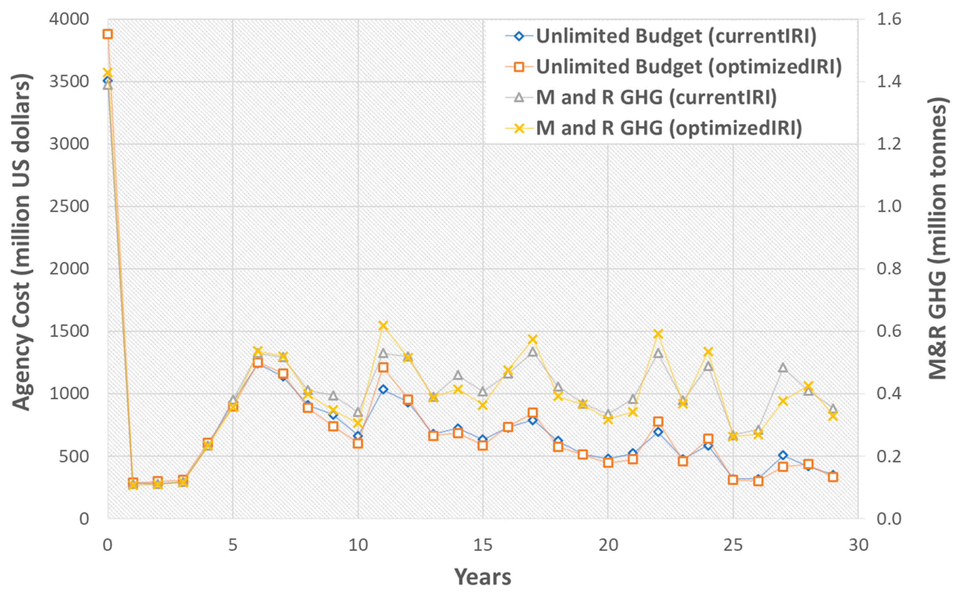
4.1. “Optimized” Triggering of Pavement Roughness to Reduce GHG
4.1.1. Study Scope, System Boundary and Functional Unit
- Unlimited budget_currentIRI—assumed no budget constraint on M and R activities. Current Caltrans decision trees were used, which trigger M and R based on predicted cracking with different treatments for different levels of cracking and faulting, or if the IRI value was 2.68 m/km (170 in/mile) or greater.
- Unlimited budget_optimizedIRI—used the same assumptions as scenario 1, except that an optimized IRI trigger value was used to trigger a treatment if not already triggered by cracking:
- Segments with passenger car equivalent (PCE) per day less than 2517—no IRI trigger value (no treatment);
- 2517 < PCE ≤ 11,704—IRI trigger value of 2.8 m/km (177 in/mile);
- 11,704 < PCE ≤ 33,908—IRI trigger value of 2.0 m/km (127 in/mile);
- 33,908 < PCE—IRI trigger value of 1.6 m/km (101 in/mile).
4.1.2. Assumptions and Limitations
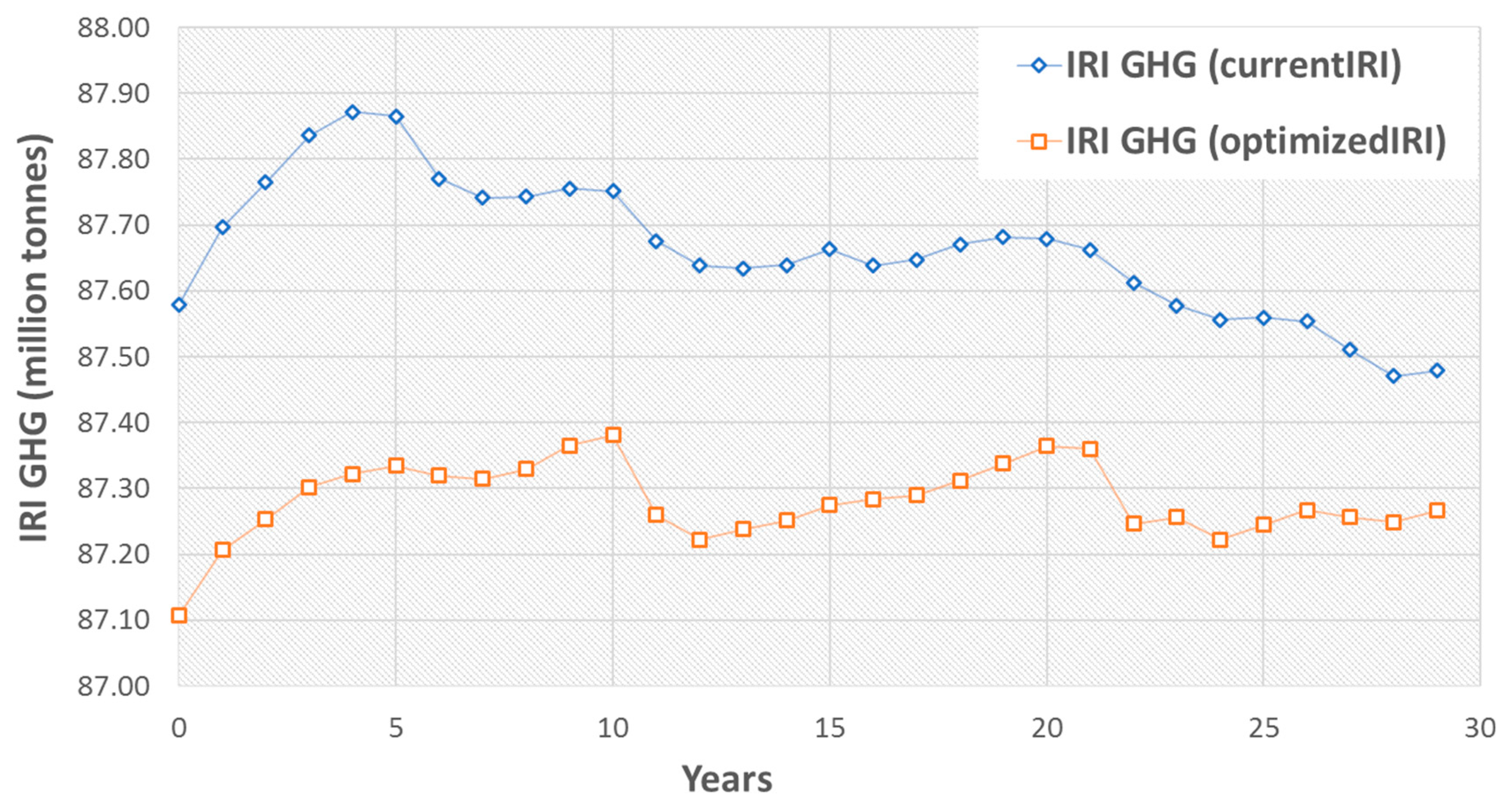
4.1.3. Results from Strategy 1
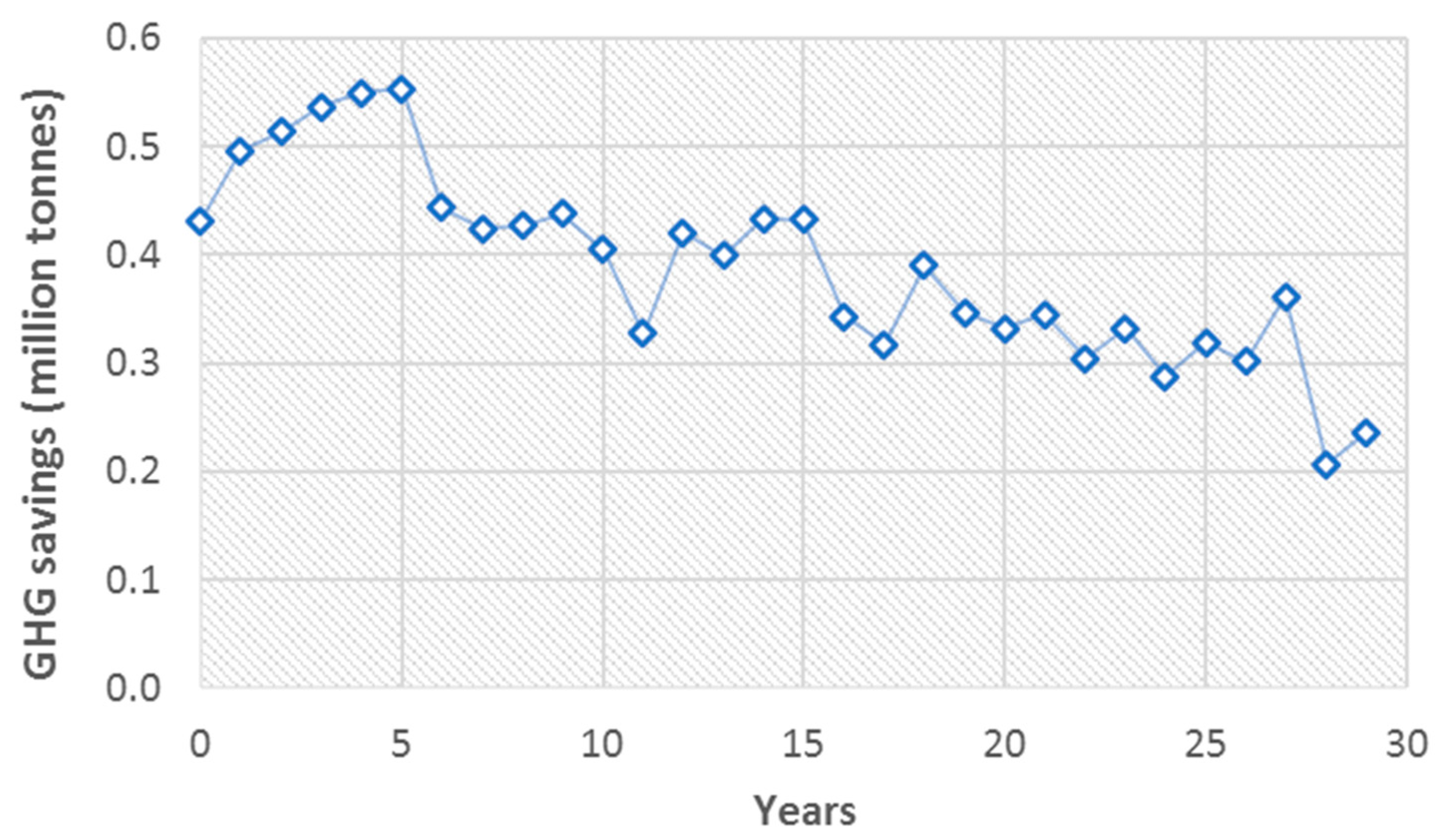
4.1.4. Abatement Potential of the Strategy
4.1.5. Time-Adjusted GHG Emissions
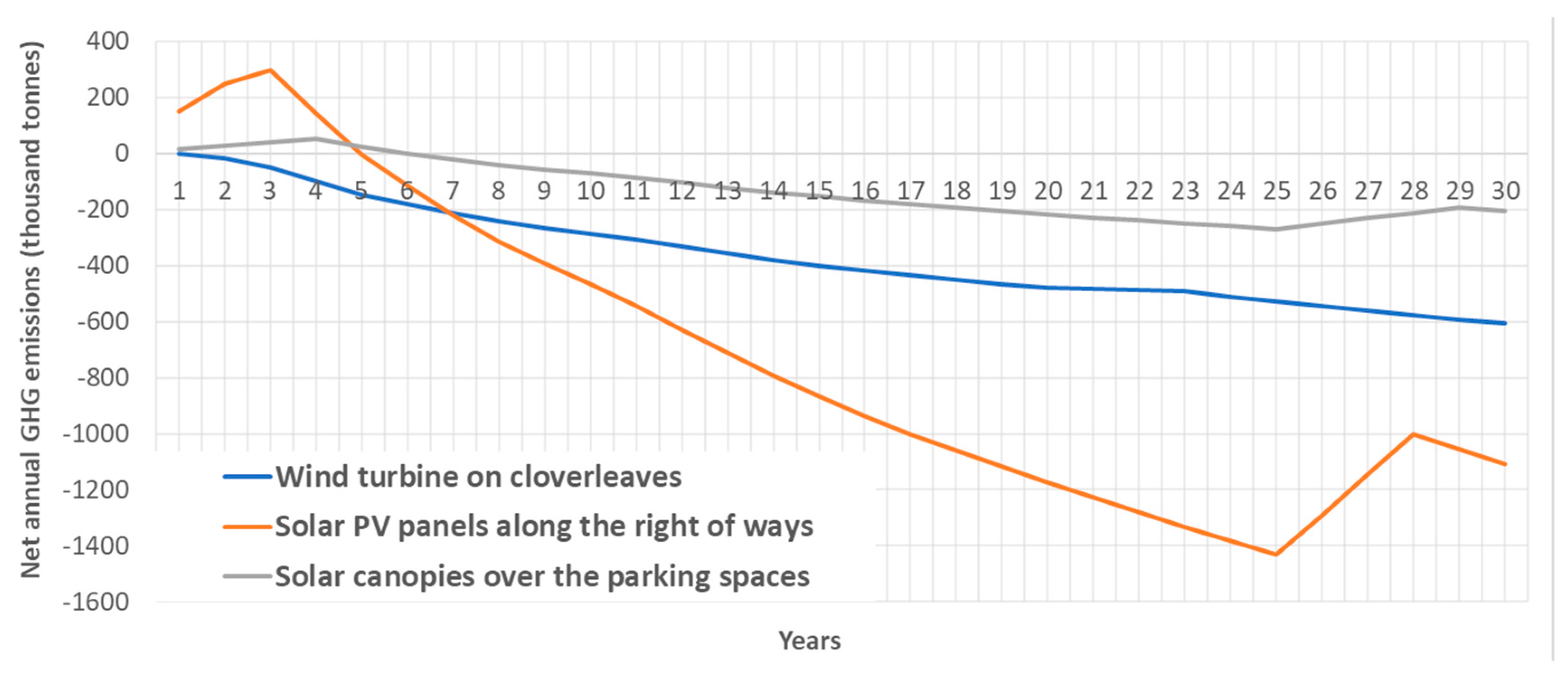
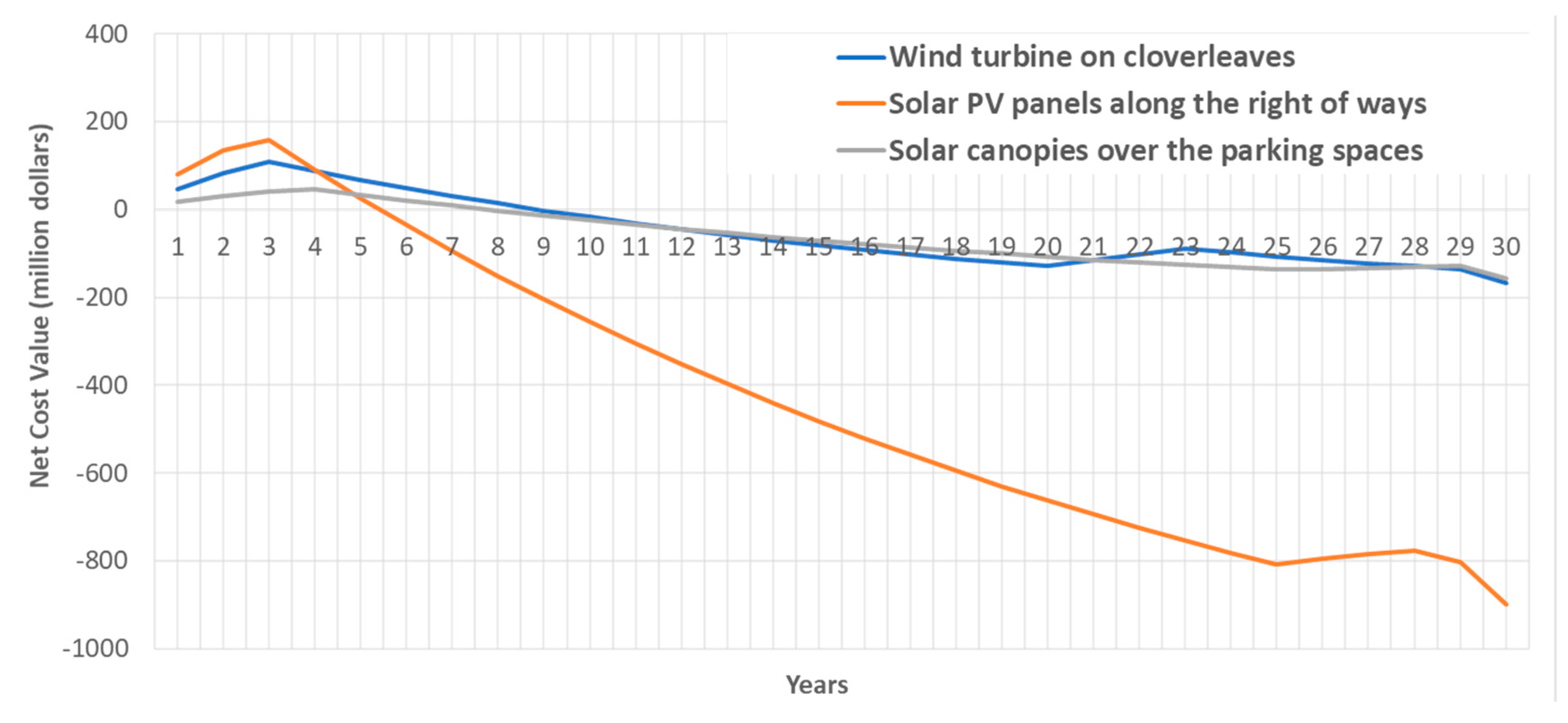
4.2. Installing Solar and Wind Energy Technologies within the State Highway Network Right-of-Way
4.2.1. Study Scope, System Boundary and Functional Unit
4.2.2. Assumptions and Limitations
- Wind energy potential—a detailed study of wind power potential was not performed, therefore the estimates of power from wind generation would likely be reduced. For this conceptual-level study the national renewable energy laboratory wind prospector mapping tool was consulted, which showed varying potential for wind energy along the three highway corridors [63].
- Additional time required for designing, planning, and permitting—the timelines for the installations of these technologies can vary widely between sites due to differences in landscape, local jurisdiction, available developers, and more. Each site would require its own design and planning, and would then require the appropriate permits. This process can take anywhere between a few months to over a year. However, this study begins the analysis once this process has been completed, and subsequently considers only the installation rate of the technologies.
- Effects of PV glare on driver safety—this is a potential drawback to PV installation along the highway as mentioned in Caltrans’ report on strategies to address climate change [60].
- Effects of wind turbine noise on the surrounding community—wind turbines are associated with low-frequency vibrations that have led to complaints from residents who live near them. While it is likely that the wind turbines will be installed in areas with low populations along these largely rural or desert wilderness highway corridors, these effects could also be experienced by drivers, though exposure would be for much shorter periods of time. The specification sheet of the Wind Energy Solutions 250 kW turbine mentions that the noise emissions generated during 8 m/s winds is 45 decibels (dB) at 100 m distance [64]. For reference, the noise level in a library is 40 dB, a quiet rural area’s noise is 30 dB (half as loud as 40 dB), and a whisper is 20 dB (half as loud as 30 dB) [65].
- Transmission losses—it is unclear whether transmission losses between the renewable energy generation site and grid are significant; they depend largely on the distance between the installed technology and the nearest grid connection.
- Effects on afternoon ramp load—electricity demand rises sharply in the afternoon and early evening as people return to their homes, and in the summer turn on air conditioning. This coincides with the decreased output of solar energy production. As solar power capacity has increased in California, and particularly from non-utility scale installations, this has led to the requirement for carbon-intensive “peaker” plants, which have often been coal-fired plants in neighboring states, to make up for this difference between supply and demand. Adding more solar energy to the grid could exacerbate this steep ramp-up of carbon-intensive peaker plants, which can result in the unintended consequence of higher carbon-intensity electricity being generated. This reduces the net benefit of supplying solar power, since it must be balanced with carbon intensive peaker plants. Wind power on the other hand will often ramp up during the afternoons along the targeted highway corridors, although it is also highly variable.
- Urban heat island reduction due to covering building roofs and parking areas—the shading of building roofs and parking areas could reduce the urban heat island effect. This could reduce the amount of energy used for cooling buildings, but could alternatively increase energy use for heating in colder months. Shading of parking lots with solar panels can lower temperatures in parked cars and reduce cooling loads, and potentially increase vehicle heating demand. For vehicles, cooling is a significantly higher energy load than heating, so the net benefit favors vehicle shading.
- Job creation in the renewable energy industry—the installation and maintenance of these technologies would generate jobs, which could be considered as a socio-economic benefit.
- Time of day pricing is not considered—some utilities charge different rates for electricity use depending on which time of the day it is consumed; alternatively, the value of generating electricity during these times is increased, while the value of generation at other times is decreased. For example, the Sacramento-based utility (Sacramento Municipal Utility District), offers time-of-day rates that are higher on summer weekdays from 5 to 8 PM, and lower throughout the rest of the day. This strategy is meant to minimize the afternoon ramp load (as explained above).
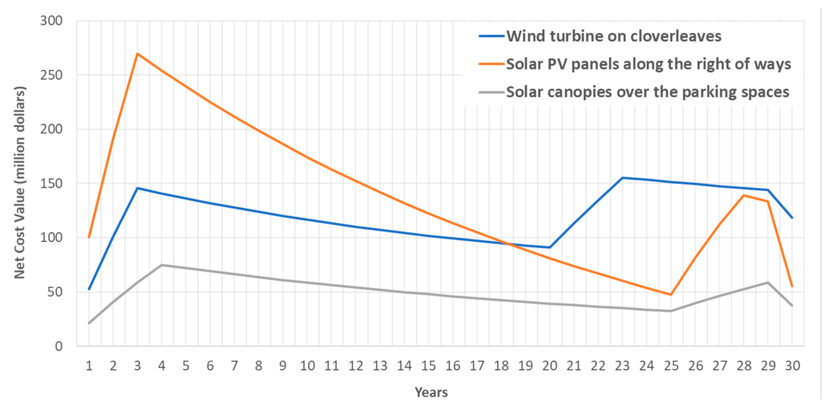
4.2.3. Results from Strategy 2
4.2.4. Abatement Potential of the Strategy
4.2.5. Time-Adjusted GHG emissions
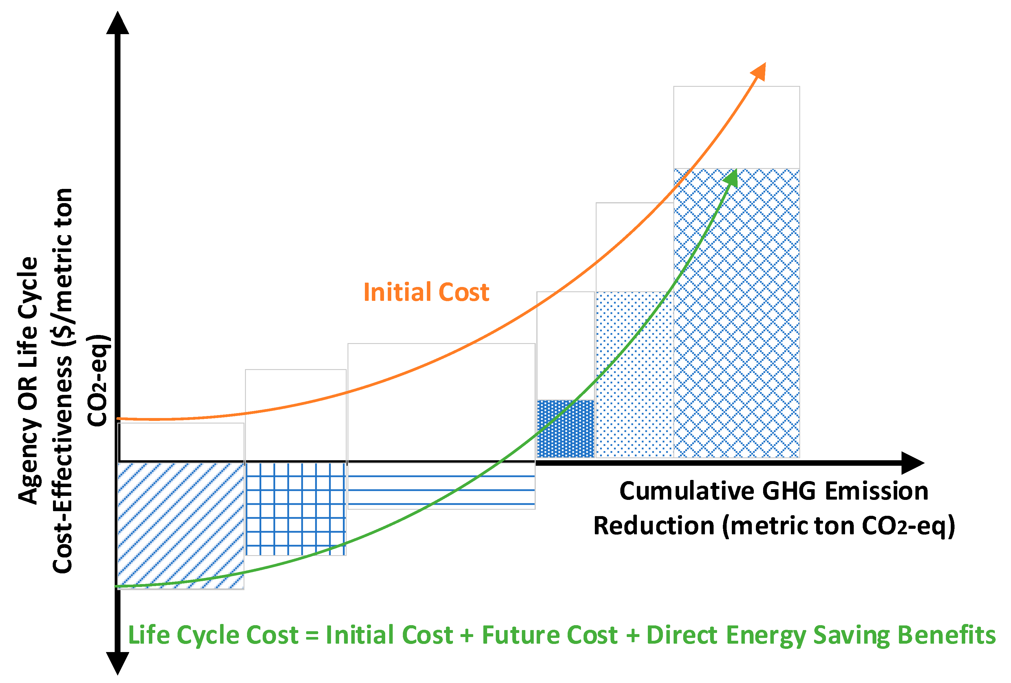
5. Supply Curve Information
6. Summary and Critiques of Supply Curves
Author Contributions
Funding
Acknowledgments
Conflicts of Interest
Appendix A

| Treatment Name | Treatment No. | Assumed Treatment Thickness, th (ft) | GHG Coefficient, (CO2-eq per ft3) | Pavement Analyzer (PA®’s) GHGmaterials&construction Coefficient 1,2 |
|---|---|---|---|---|
| “Do-Nothing” | 0 | 0 | 0 | 0 |
| Fog Seal, Slurry Seal, Chip Seal, Seal Coat-Corrective, microsurfacing, Seal Coat-Preventive | 209, 210, 211, 194, 212, 275 | 0.05 | 0.006673 a | 21.14 |
| HMA Thin Overlay (th ≤ 0.10 ft), HMA Thin Overlay-Preventive | 195, 276 | 0.1 | 0.006673 a | 42.28 |
| HMA Medium Overlay (0.10 < th < 0.25 ft) | 196 | 0.2 | 0.006673 a | 84.56 |
| HMA Thick Overlay (th3 0.25 ft) | 197 | 0.4 | 0.006673 a | 169.12 |
| Full Depth Reclamation (FDR) | 199 | 0.57 | 0.006673 a,b | 241 |
| Cold In-place Recycling (CIR), Cold In-Place Recycling-Class 3 | 200, 277 | 0.37 | 0.006673 a,b | 156.44 |
| Seal Cracks (assumed to have no GHG) | 201 | 0 | 0.006673 | 0 |
| Hot In-Place Recycling (HIPR) | 223 | 0.37 | 0.006673 a,b | 156.44 |
| Mill and Fill | 285 | 0.1 | 0.006673 c | 42.28 |
| Treatment Name | Treatment No. | Assumptions | Assumed Treatment Thickness, th | GHG coefficient, g (CO2-eq per ft3) | GHGmaterials&construction coefficient, g (CO2-eq per ft3) |
|---|---|---|---|---|---|
| Do Nothing | 0 | 0 | |||
| Crack Seat and Overlay (CSOL) | 202 | Place one HMA overlay thickness over cracked and seated JPCP slabs | 0.49 ft HMA | 0.006673 a | 207.17 |
| PCC Lane Replacement | 203 | Assume slabs (rapid strength concrete) and base replaced. Assume slab thickness and base thickness to be 0.75 ft each. Assume the newly placed base to contribute half of the GHG contributed by the slab. | 0.75 ft PCC, 0.75 ft Base | 0.013760 b | 980.81 |
| Grind PCC for Smoothness-CAPM, Grinding-Preventive, Grinding (poor ride only)-Corrective | 204, 283, 284 | Assume grinding depth to be equal to 0.375 inch (0.03125 ft) | 0.03125 ft | 0.00329 | 6.514 |
| Grind/Replace Slabs-CAPM b | 205 | Two treatments. Slab thickness 0.75 ft. Grinding depth 0.03125 ft | 0.75 ft PCC slab, and 0.03125 ft grinding | 0.01589 for slab replacement, 0.00329 for grinding | 755.09 for slab replacement to be multiplied by slab percentage needing replacement. For grinding the coefficient is 6.154. (GHG Calculation in groovy script “GHG Calculation”) |
| Slab Replacement-Corrective c | 206 | Two treatments. Slab thickness 0.75 ft. Grinding depth 0.03125 ft. | 0.75 ft and 0.03125 ft | 0.01589 | 755.09 to be multiplied by percentage of slabs replaced in the lane mile (GHG Calculation and GHG factors in groovy script “GHG Calculation”) |
| Groove PCC pavement | 222 | 0.03125 ft (assumed like grinding) | 0.00329 | 6.154 | |
| PCC Overlay | 226 | 1.12 ft back- calculated from 980.81 and 0.013760 for concrete slab GHG factor. | 980.81 | ||
| CRCP Lane Replacement | 247 | Similar to JPCP lane replacement | 0.75 ft PCC, 0.75 ft Base | 0.013760 b | 980.81 |
| Dowel Bar Retrofit | 249 | No information available at the moment. |
| Vehicle Classification | Roughness Factor (f) | Constant (C) |
|---|---|---|
| Car, Pickup Truck | 0.0098 | 0.36562 |
| Two-Axle Truck | 0.00994 | 1.09834 |
| Three-Axle Truck | 0.02 | 1.80147 |
| Four-Axle Truck | 0.03317 | 2.62255 |
| Five-Axle Truck | 0.03509 | 2.86596 |
| 1. The new factors are based on T. Wang’s factors [43]. | ||
| 2. The factors are used to calculate the CO2 quantity in tonnes per “1000 miles” driven by ONE vehicle of the classes given below. | ||
| 3. Factors weight-averaged for asphalt and concrete surfaced pavements using 74% versus 26% | ||
| 4. The original equation for CO2 calculation assumed effect of IRI and mean profile depth (MPD). The MPD was removed from the equations because it was found to have a small effect compared to roughness. The GHG emission was assumed to be solely affected by the rolling resistance associated with IR. | ||
| 5. The final equation for CO2 quantity is: [CO2] = f*IRI + C, where IRI in m/km and [CO2] in tonnes. | ||
| 6. Example calculation: one passenger car driving over a pavement with IRI of 1 m/km (63 in/mile) will produce 0.00980 × 1 + 0.36562 = 0.37541 tonnes per 1000 miles driven (i.e., 1000 VMT). | ||
| 7. If VMT is calculated from directional ADT, then each vehicle class will have its own ADT. The ADT must also be split per lane and then per segment being analyzed. Using segment length Li, ADT on that segment is ADTi, and then VMTi for that segment is ADTi × Li. This will be done for each vehicle class. Then factors f and C for each class are used with each vehicle class. The CO2 is calculated per each one vehicle of each type and then multiplied by VMTi of each vehicle class and summed over. | ||
| Categories | Data Sources | Data Quality | |||||||
|---|---|---|---|---|---|---|---|---|---|
| Reliability | Geography | Time | Technology | Completeness | Reproducibility | Representativeness | Uncertainty | ||
| Data Type | |||||||||
| Lane-miles of state network | Caltrans/PaveM | Very Good | US | Good | Very Good | Very Good | Yes | Yes | Low |
| Pavement types | Caltrans/PaveM | Very Good | US | Good | Very Good | Very Good | Yes | Yes | Low |
| Average pavement thicknesses | Caltrans/PaveM | Very Good | US | Good | Very Good | Very Good | Yes | Yes | Low |
| Annual traffic | Caltrans/PaveM | Very Good | US | Good | Very Good | Very Good | Yes | Yes | Low |
| % vehicle types/class | Caltrans/PaveM | Very Good | US | Good | Very Good | Very Good | Yes | Yes | Low |
| Pavement performance equations (IRI, cracking) | Lea et al. [44] implemented in PaveM | Good | US | Very Good | Very Good | Very Good | Yes | Yes | High |
| Pavement condition (IRI, cracking) | Caltrans APCS data | Very Good | US | Good | Very Good | Very Good | Yes | Yes | Low |
| LCA Related | |||||||||
| Asphalt | Athena Institute [71] | Good | CDN/US | Poor | Very Good | Poor | Yes | Yes | High |
| Cement | Marceau [72] | Good | US | Poor | Very Good | Poor | Yes | Yes | High |
| Other materials | Wang 2013/Stripple [45,69] | Good | SE/US | Poor | Very Good | Fair | Yes | Yes | High |
| Other materials | EcoInvent [70] | Good | SW | Poor | Very Good | Fair | Yes | Yes | High |
| Other materials | USLCI [71] | Good | US | Poor | Very Good | Fair | Yes | Yes | High |
| Materials and treatments factors | PaveM | Good | US | Fair | Very Good | Fair | Yes | Yes | Low |
| Cost Related | |||||||||
| Treatment agency costs | PaveM | Very Good | US | Good | Very Good | Good | Yes | Yes | Low |
| Question Number | Question | Answer |
|---|---|---|
| 1. | Define change |
|
| 2. | Define the state of readiness of the change of technology (using approach adapted from NASA) |
|
| 3. | Define system in which change occurs |
|
| 4. | Will the market change or is it just changes in market share? | Not applicable. |
| 5. | Who is responsible for change? | Caltrans |
| 6. | Who is responsible for implementing change? | Caltrans |
| 7. | Who pays for change | State government |
| 8. | What will drive change (X) |
|
| 9. | What will the change do to these other environmental indicators | LCA will answer
|
| 10. | What are the performance metrics in addition to GHG reduction and cost? |
|
| 11. | Supply curve calculation questions: |
|
Appendix B
| Categories | Data Sources | Data Quality | |||||||
|---|---|---|---|---|---|---|---|---|---|
| Reliability | Geography | Time | Technology | Completeness | Reproducibility | Representativeness | Uncertainty | ||
| Data Type | |||||||||
| Annual solar energy generation | Sendy [90] | Fair | US | Good | Very Good | Fair | Yes | Yes | Low |
| Solar PV degradation rate | Hsu et al. [83] | Very Good | US | Fair | Very Good | Very Good | Yes | Yes | Low |
| Annual wind energy generation | Smoucha et al. [74] | Very Good | US | Fair | Very Good | Very Good | Yes | Yes | Low |
| Turbine degradation rate | Staffel and Green [77] | Very Good | US | Good | Very Good | Very Good | Yes | Yes | Low |
| LCA Related | |||||||||
| Wind Turbine | Smoucha et al. [74] | Good | EU | Fair | Very Good | Very Good | Yes | Yes | Low |
| Solar Panel | Hsu et al. [83] | Very Good | US | Fair | Very Good | Very Good | Yes | Yes | Low |
| Electricity | US EIA [84] | Very Good | US | Good | Very Good | Very Good | Yes | Yes | Low |
| Steel | EcoInvent [70] | Good | Global | Fair | Very Good | Fair | Yes | Yes | High |
| Cement Concrete | Saboori et al. [91] | Very Good | US | Very Good | Very Good | Very Good | Yes | Yes | Low |
| Cost Related | |||||||||
| Wind Turbine | Wiser and Bolinger [82] | Very Good | US | Very Good | Very Good | Good | Yes | Yes | Low |
| Solar Panel | US EIA [84] | Good | US | Good | Very Good | Good | Yes | Yes | High |
| Electricity | US EIA [84] | Very Good | US | Good | Very Good | Good | Yes | Yes | Low |
| Steel | Focus Economics | Good | US | Very Good | Very Good | Good | Yes | Yes | Low |
| Solar Carport | Solar Electric Supply Inc. [89] | Very Good | US | Very Good | Very Good | Good | Yes | Yes | Low |
| Question Number | Question | Answer |
|---|---|---|
| 1. | Define change |
|
| 2. | Define the state of readiness of the change of technology (using approach adapted from NASA) | Solar canopies over parking spaces: TRL 9: actual system proven in operational environment elsewhere or less-than-full market penetration. Wind turbines in interchanges and solar panel along right-of-ways: TRL 5 and 6: technology validated and demonstrated in relevant environment at less than full scale. |
| 3. | Define system in which change occurs | Caltrans owned and operated state highway network and other land/property assets. Cost to be carried within existing budgets unless other funds found, bonds, CAP and Trade, or additional state funding increase in budget. Budget constraint optimization and unconstrained optimization. Cannot be the only criteria for funding. |
| 4. | Will the market change or is it just changes in market share? | No |
| 5. | Who is responsible for change? | Caltrans. State transport agency, CTC, legislature, energy commission, CPUC |
| 6. | Who is responsible for implementing change? | Caltrans |
| 7. | Who pays for change |
|
| 8. | What will drive change (X) |
|
| 9. | What will the change do to these other environmental indicators | LCA will answer
|
| 10. | What are the performance metrics in addition to GHG reduction and cost? |
|
| 11. | Supply curve calculation questions: |
|
References and Notes
- Hulme, P.E. Adapting to climate change: Is there scope for ecological management in the face of a global threat? J. Appl. Ecol. 2005, 42, 784–794. [Google Scholar] [CrossRef]
- Maclean, I.M.; Wilson, R.J. Recent ecological responses to climate change support predictions of high extinction risk. Proc. Natl. Acad. Sci. USA 2011, 108, 12337–12342. [Google Scholar] [CrossRef] [PubMed]
- McMichael, A.J.; Woodruff, R.E. Climate Change and Human Health; Oliver, J.E., Ed.; Encyclopedia of World Climatology 2005. Encyclopedia of Earth Sciences Series; Springer: Dordrecht, The Netherlands, 2005; pp. 209–213. [Google Scholar]
- Rice, S.A. Human health risk assessment of CO2: Survivors of acute high-level exposure and populations’ sensitive to prolonged low-level exposure. Environments 2014, 3, 7–15. [Google Scholar]
- Kampa, M.; Castanas, E. Human health effects of air pollution. Environ. Pollut. 2008, 151, 362–367. [Google Scholar] [CrossRef] [PubMed]
- Lave, L.B.; Seskin, E.P. Air Pollution and Human Health, 1st ed.; Taylor & Francis Group, RFF Press: New York, NY, USA, 2013. [Google Scholar]
- Colvile, R.N.; Hutchinson, E.J.; Mindell, J.S.; Warren, R.F. The transport sector as a source of air pollution. Atmos. Environ. 2001, 35, 1537–1565. [Google Scholar] [CrossRef]
- Hooftman, N.; Oliveira, L.; Messagie, M.; Coosemans, T.; Van Mierlo, J. Environmental analysis of petrol, diesel and electric passenger cars in a Belgian urban setting. Energies 2016, 9, 84. [Google Scholar] [CrossRef]
- Marseglia, G.; Rivieccio, E.; Medaglia, C.M. The dynamic role of Italian energy strategies in the worldwide scenario. Kybernetes 2019, 48, 636–649. [Google Scholar] [CrossRef]
- Shayegh, S.; Sanchez, D.L.; Caldeira, K. Evaluating relative benefits of different types of R&D for clean energy technologies. Energy Policy 2017, 107, 532–538. [Google Scholar]
- Sovacool, B.K.; Geels, F.W. Further reflections on the temporality of energy transitions: A response to critics. Energy Res. Soc. Sci. 2016, 22, 232–237. [Google Scholar] [CrossRef]
- United Nations. Paris Agreement. Conference of the Parties to the United Nations Framework Convention on Climate Change. 2015. Available online: https://treaties.un.org/Pages/ViewDetails.aspx?src=TREATY&mtdsg_no=XXVII-7-d&chapter=27&lang=_en&clang=_en (accessed on 30 May 2019).
- California State Legislature. Assembly Bill 32, California Global Warming Solutions Act of 2006. 2006. California, USA.
- The Climate Mobilization. Oakland, CA Declares Climate Emergency. 2018. Available online: https://www.theclimatemobilization.org/blog/2018/10/31/oakland-ca-declares-climate-emergency (accessed on 30 May 2019).
- County Climate Coalition. 2018. Available online: https://www.climaterealityproject.org/climatecoalition (accessed on 30 May 2019).
- California Air Resources Board. GHG Current California Emission Inventory Data. 2019. Available online: https://ww2.arb.ca.gov/ghg-inventory-data (accessed on 24 September 2019).
- Ritchie, H.; Roser, M. CO2 and Greenhouse Gas Emissions. Published online at OurWorldInData.org. 2019. Available online: https://ourworldindata.org/co2-and-other-greenhouse-gas-emissions (accessed on 24 September 2019).
- FHWA. 2013 Pocket Guide to Transportation; Federal Highway Administration: Washington, DC, USA, 2013.
- FHWA. Highway Statistics; Federal Highway Administration: Washington, DC, USA, 2012.
- FHWA. Travel Monitoring. Federal Highway Administration, 2017. Available online: https://www.fhwa.dot.gov/policyinformation/travel_monitoring/historicvmt.cfm (accessed on 29 May 2019).
- FHWA. Towards Sustainable Pavement Systems: A Reference Document. FHWA-HIF-15-002, February 2015. Available online: http://www.fhwa.dot.gov/pavement/sustainability/ref_doc.cfm (accessed on 29 May 2019).
- BTS & FHWA. Freight Facts and Figures 2013. Bureau of Transportation Statistics and Federal Highway Administration, FHWA-HOP-14-004. Washington, DC. January 2014. Available online: http://www.ops.fhwa.dot.gov/freight/freight_analysis/nat_freight_stats/docs/13factsfigures/pdfs/fff2013_highres.pdf (accessed on 29 May 2019).
- BLS. National Industry-Specific Occupational Employment and Wage Estimates, Bureau of Labor Statistics. 2014. NAICS 237300—Highway, Street, and Bridge Construction. Department of Labor, Washington, DC. Available online: http://www.bls.gov/oes/current/naics4_237300.htm#startcontent (accessed on 29 May 2019).
- CBO. Spending on Infrastructure and Investment. Congressional Budget Office, 2017. Available online: https://www.cbo.gov/publication/52463 (accessed on 29 May 2019).
- FHWA. Motor-Fuel Use—2015. Federal Highway Administration, 2017. Available online: https://www.fhwa.dot.gov/policyinformation/statistics/2015/mf21.cfm (accessed on 29 May 2019).
- EPA. U.S. Transportation Sector Greenhouse Gas Emissions 1990–2016. US Environmental Protection Agency, 2018. Available online: https://nepis.epa.gov/Exe/ZyPDF.cgi?Dockey=P100USI5.pdf (accessed on 29 May 2019).
- CARB. Annual State-Wide Greenhouse Gas Inventory. California Air Resources Board, 2018. Available online: https://www.arb.ca.gov/cc/inventory/inventory.htm (accessed on 7 April 2019).
- CARB. California Greenhouse Gas Emissions Emissions for 2000 to 2016 Trends of Emissions and Other Indicators. California Air Resources Board, 2018. Available online: https://www.arb.ca.gov/cc/inventory/pubs/reports/2000_2016/ghg_inventory_trends_00-16.pdf (accessed on 5 March 2019).
- Givoni, M.; Macmillen, J.; Banister, D.; Feitelson, E. From Policy Measures to Policy Packages. Transp. Rev. 2013, 33, 1–20. [Google Scholar] [CrossRef]
- Taeihagh, A.; Givoni, M.; Bañares-Alcántara, R. Which policy first? A networkcentric approach for the analysis and ranking of policy measures. Environ. Plan. B 2013, 40, 595–616. [Google Scholar] [CrossRef]
- Harvey, J.T.; Meijer, J.; Ozer, H.; Al-Qadi, I.; Saboori, A.; Kendall, A. Pavement Life-Cycle Assessment Framework. Federal Highway Administration 2016. FHWA-HIF-16-014. Available online: http://www.fhwa.dot.gov/pavement/sustainability/hif16014.pdf (accessed on 20 May 2019).
- Caltrans. Life-Cycle Cost Analysis Procedure Manual. California Department of Transportation, 2013. Available online: http://www.dot.ca.gov/hq/maint/Pavement/Offices/Pavement_Engineering/LCCA_Docs/LCCA_25CA_Manual_Final_Aug_1_2013_v2.pdf (accessed on 29 May 2019).
- Kendall, A. Time-adjusted global warming potentials for LCA and carbon footprints. Int. J. Life Cycle Assess. 2012, 17, 1042–1049. [Google Scholar] [CrossRef]
- Creyts, J.; Durkach, A.; Nyquist, S.; Ostrowski, K.; Stephenson, J. Reducing U.S. Greenhouse Gas Emissions: How Much at What Cost? McKinsey & Company for the Conference Board. U.S. Greenhouse Gas Abatement Mapping Initiative 2007. Available online: https://www.mckinsey.com/business-functions/sustainability/our-insights/reducing-us-greenhouse-gas-emissions (accessed on 29 May 2019).
- Lutsey, N.P.; Sperling, D. Greenhouse gas mitigation supply curve for the United States for transport versus other sectors. Transp. Res. Part D 2009, 14, 222–229. [Google Scholar] [CrossRef]
- Lutsey, N.P. Prioritizing Climate Change Mitigation Alternatives: Comparing Transportation Technologies to Options in Other Sectors; Research Report UCD-ITS-RR-08-15; Institute of Transportation Studies, University of California Davis: Davis, CA, USA, 2008. [Google Scholar]
- ISO 14044. Environmental Management: Life Cycle Assessment—Requirements and Guidelines; International Organization for Standardization: Geneva, Switzerland, 2006. [Google Scholar]
- NASA. Technology Readiness Level. The National Aeronautics and Space Administration, 2012. Available online: https://www.nasa.gov/directorates/heo/scan/engineering/technology/txt_accordion1.html (accessed on 29 May 2019).
- Bare, J. TRACI 2.0: The Tool for the Reduction and Assessment of Chemical and Other Environmental Impacts 2.0. Clean Technol. Environ. 2011, 13, 687–696. [Google Scholar] [CrossRef]
- US EPA. Tool for the Reduction and Assessment of Chemical and Other Environmental Impacts (TRACI) User’s Manual; Document ID: S-10637-OP-1-0; Environmental Protection Agency: Washington, DC, USA, 2012.
- Evans, L.R.; MacIsaac, J.D., Jr.; Harris, J.R.; Yates, K.; Dudek, W.; Holmes, J.; Popio, J.; Rice, D.; Salaani, M. NHTSA Tire Fuel Efficiency Consumer Information Program Development: Phase 2—Effects of Tire Rolling Resistance Levels on Traction, Treadwear, and Vehicle Fuel Economy; National Highway Traffic Safety Administration: East Liberty, OH, USA, 2009.
- Wang, T.; Harvey, J.; Kendall, A. Reducing greenhouse gas emissions through strategic management of highway pavement roughness. Environ. Res. Lett. 2014, 9, 034007. [Google Scholar] [CrossRef]
- Wang, T.; Harvey, J.T.; Kendall, A. Network-Level Life-Cycle Energy Consumption and Greenhouse Gas from CAPM Treatments. University of California Pavement Research Center. UCPRC-RR-2014-05, 2015. Available online: http://www.ucprc.ucdavis.edu/PDF/UCPRC-RR-2014-05.pdf (accessed on 12 March 2018).
- Lea, J.D.; Harvey, J.; Tseng, E. Aggregating and Modeling Automated Pavement Condition Survey Data for Flexible Pavements for Use in Pavement Management. Transp. Res. Rec. 2014, 2455, 84–97. [Google Scholar] [CrossRef]
- Wang, T.; Lee, I.S.; Harvey, J.T.; Kendall, A.; Lee, E.B.; Kim, C. UCPRC Life Cycle Assessment Methodology and Initial Case Studies on Energy Consumption and GHG Emissions for Pavement Preservation Treatments with Different Rolling Resistance. UCPRC-RR-2012-02, 2012, Davis and Berkeley, CA. Available online: http://www.ucprc.ucdavis.edu/PDF/UCPRC-RR-2012-02.pdf (accessed on 12 March 2018).
- Wang, T.; Lee, I.S.; Kendall, A.; Harvey, J.; Lee, E.B.; Kim, C. Life cycle energy consumption and GHG emission from pavement rehabilitation with different rolling resistance. J. Clean. Prod. 2012, 33, 86–96. [Google Scholar] [CrossRef]
- Wang, T.; Harvey, J.T.; Lea, J.D.; Kim, C. Impact of Pavement Roughness on Vehicle Free-Flow Speed. UCPRC-TM-2013-04, 2013. Available online: http://www.ucprc.ucdavis.edu/PDF/UCPRC-TM-2013-04.pdf (accessed on 12 March 2018).
- Wang, T.; Harvey, J.; Lea, J.D.; Kim, C. Impact of pavement roughness on vehicle free-flow speed. J. Transp. Eng. 2014, 140, 04014039. [Google Scholar] [CrossRef]
- Fontaras, G.; Zacharof, N.; Biagio, C. Fuel consumption and CO2 emissions from passenger cars in Europe—Laboratory versus real-world emissions. Prog. Energy Combust. Sci. 2017, 60, 97–131. [Google Scholar] [CrossRef]
- Franzese, O.; Davidson, D. Effect of Weight and Roadway Grade on the Fuel Economy of Class-8 Trucks; Report ORNL/TM-2011/471; Oak Ridge National Laboratory: Oak Ridge, TN, USA, 2011.
- West, B.H.; McGill, R.N.; Sluder, S. Development and Validation of Light-Duty Vehicle Modal Emissions and Fuel Consumption Values for Traffic Models; FHWA-RD-99-068; Federal Highway Administration (FHWA): Washington, DC, USA, 1999.
- California Air Resources Board. 2017. Mobile Source Emission Inventory the EMission FACtors (EMFAC) Model Web Database, Vehicle Data for Calendar Year 2015. Available online: https://www.arb.ca.gov/emfac/2017/ (accessed on 27 September 2019).
- Energy 2016. Fact #997, October 2, 2017: Average Age of Cars and Light Trucks Was Almost 12 Years in 2016. Available online: https://www.energy.gov/eere/vehicles/articles/fact-997-october-2-2017-average-age-cars-and-light-trucks-was-almost-12-years (accessed on 25 September 2019).
- California Air Resources Board 2018. California’s Sustainable Communities and Climate Protection Act. Report. Available online: https://ww2.arb.ca.gov/sites/default/files/2018-11/Final2018Report_SB150_112618_02_Report.pdf (accessed on 25 September 2019).
- Federal Highway Administration. 2010 Status of the Nation’s Highways, Bridges, and Transit 2010. Conditions & Performance. Chapter 1: Household Travel in America. Available online: https://www.fhwa.dot.gov/policy/2010cpr/chap1.cfm (accessed on 27 September 2019).
- Life Cycle Cost Analysis Procedures Manual; California Department of Transportation: Sacramento, CA, USA, 2010.
- California Air Resources Board. 2019. California Cap-and-Trade Program, Summary of California-Quebec Joint Auction Settlement Prices and Results. Updated May, 2019. Available online: https://www.arb.ca.gov/cc/capandtrade/auction/results_summary.pdf (accessed on 31 May 2019).
- Fox, D.; Matsuo, J.; Miner, D. Caltrans Sustainability Roadmap 2018–2019. Caltrans. Progress Report and Plan Update on Meeting the Governor’s Sustainability Goals for State Departments 2018. Available online: https://green.ca.gov/Documents/CALTRANS/CALTRANS_2018-2019_Roadmap_Complete_Document.pdf (accessed on 12 March 2019).
- Tavares, T. Sacramento Solar Highway. Presentation: Solar Installations with the State’s Right of Way. Available online: http://www.dot.ca.gov/hq/transprog/ctcliaison/2010/0610/PP_T138_2.4c1_SolarInstallations.pdf (accessed on 12 March 2019).
- ICF International. Caltrans Activities to Address Climate Change Reducing Greenhouse Gas Emissions and Adapting to Impacts 2013. Available online: http://www.dot.ca.gov/hq/tpp/offices/orip/climate_change/documents/Caltrans_ClimateChangeRprt-Final_April_2013.pdf (accessed on 29 May 2019).
- U.S. Energy Information Administration, 2018. Electric Power Monthly with Data for December 2017. Available online: https://www.eia.gov/electricity/monthly/ (accessed on 12 March 2019).
- CPUC. Net Energy Metering (NEM). California Public Utilities Commissions, 2019. Available online: http://www.cpuc.ca.gov/general.aspx?id=3800 (accessed on 12 March 2019).
- National Renewable Energy Laboratory. Wind Prospector Mapping Tool. 2019. Available online: https://maps.nrel.gov/wind-prospector (accessed on 31 May 2019).
- WES 250 Specification Sheet. Wind Energy Solutions, 2019. Available online: https://windenergysolutions.nl/turbines/windturbine-wes-250/#pdfForm (accessed on 12 March 2019).
- IAC Acoustics. Comparative Examples of Noise Levels 2019. Available online: http://www.industrialnoisecontrol.com/comparative-noise-examples.htm (accessed on 12 March 2019).
- Kesicki, F.; Akins, P. Marginal abatement cost curves: A call for caution. Clim. Policy 2012, 12, 219–236. [Google Scholar] [CrossRef]
- Huang, S.; Lopin, K.; Chou, K.L. The applicability of marginal abatement cost approach: A comprehensive review. J. Clean. Prod. 2016, 127, 59–71. [Google Scholar] [CrossRef]
- Morris, J.; Patlsev, S.; Reilly, J. Marginal Abatement Costs and Marginal Welfare Costs for Greenhouse Gas Emissions Reductions: Results from the EPPA Model. Environ. Model. Assess. 2012, 17, 325. [Google Scholar] [CrossRef]
- Stripple, H. Life Cycle Assessment of Road: A Pilot Study for Inventory Analysis, 2nd ed.; VTI: Linköping, Sweden, 2001. [Google Scholar]
- Swiss Centre for Life Cycle Inventories. EcoInvent 2011; Swiss Centre for Life Cycle Inventories: Dubendorf, Switzerland, 2011. [Google Scholar]
- National Renewable Energy Laboratory. U.S. Life Cycle Inventory Database; National Renewable Energy Laboratory: Golden, CO, USA, 2011.
- Marceau, M.L.; Nisbet, M.A.; VanGeem, M.G. Life Cycle Inventory of Portland Cement Manufacture; SN2095b 2006; Portland Cement Association: Skokie, IL, USA, 2006. [Google Scholar]
- Basheer, I. Statewide Pavement Life Cycle Assessment with Caltrans’ Pavement Management System PaveM. In Proceedings of the International Symposium on Pavement, Roadway, and Bridge Life Cycle Assessment 2020, Sacramento, CA, USA, 3–6 June 2020. [Google Scholar]
- Smoucha, E.A.; Fitzpatrick, K.; Buckingham, S.; Knox, O.G.G. Life Cycle Analysis of the Embodied Carbon Emissions from 14 Wind Turbines with Rated Powers between 50 Kw and 3.4 Mw. J. Fundam. Renew. Energy Appl. 2016, 6, 211. [Google Scholar] [CrossRef]
- Razdan, P.; Garrett, P. Life Cycle Assessment of Electricity Production from an Onshore V110-2.0MW Wind Plant. 2015, Vestas. Available online: https://www.vestas.com/~/media/vestas/about/sustainability/pdfs/lcav11020mw181215.pdf (accessed on 12 March 2019).
- U.S. Energy Information Administration, 2015. Wind Generation Seasonal Patterns Vary across the United States. Available online: https://www.eia.gov/todayinenergy/detail.php?id=20112# (accessed on 12 March 2019).
- Staffell, I.; Green, R. How does wind farm performance decline with age? Renew. Energy 2016, 66, 775–786. [Google Scholar] [CrossRef]
- Martínez, E.; Sanz, F.; Pellegrini, S.; Jiménez, E.; Blanco, J. Life-cycle assessment of a 2-MW rated power wind turbine: CML method. Int. J. Life Cycle Assess. 2009, 14, 52–63. [Google Scholar] [CrossRef]
- Haapala, K.R.; Prempreeda, P. Comparative life cycle assessment of 2.0 MW wind turbines. Int. J. Sustain. Manuf. 2014, 3, 170–185. [Google Scholar] [CrossRef]
- Denholm, P.; Hand, M.; Jackson, M.; Ong, S. Land-Use Requirements of Modern Wind Power Plants in the United States 2009. Available online: http://www.osti.gov/bridge (accessed on 12 March 2019).
- Thomson, R.C.; Harrison, G.P. Life Cycle Costs and Carbon Emissions of Onshore Wind Power. ClimateXChange. 2015. Available online: https://www.climatexchange.org.uk/media/1463/main_report_-_life_cycle_costs_and_carbon_emissions_of_onshore_wind_power.pdf (accessed on 12 March 2019).
- Wiser, R.; Bolinger, M. 2017 Wind Technologies Market Report; US Department of Energy, Office of Energy Efficiency and Renewable Energy: Washington, DC, USA, 2018.
- Hsu, D.D.; O’Donoughue, P.; Fthenakis, V.; Heath, G.A.; Kim, H.C.; Sawyer, P.; Choi, J.; Turney, D.E. Life Cycle Greenhouse Gas Emissions of Crystalline Silicon Photovoltaic Electricity Generation. J. Ind. Ecol. 2012, 16, 122–135. [Google Scholar] [CrossRef]
- Sendy, A. How Much Electricity Do Solar Panels Produce Per Day in Each State? Solar-Estimate. Available online: https://www.solar-estimate.org/solar-panels-101/how-much-do-solar-panels-produce (accessed on 12 March 2019).
- U.S. Energy Information Administration. Levelized Cost and Levelized Avoided Cost of New Generation Resources in the Annual Energy Outlook 2018; U.S. Energy Information Administration: Washington, DC, USA, 2018.
- Pacca, S.; Sivaraman, D.; Keoleian, G.A. Parameters affecting the life cycle performance of PV technologies and systems. Energy Policy 2007, 35, 3316–3326. [Google Scholar] [CrossRef]
- Velizadeh, S.; (Park & Ride Inventory 2019). Personal communication, 2019.
- Caltrans. Park & Ride Inventory 2018. Available online: http://www.dot.ca.gov/trafficops/tm/docs/park_ride_inventory_2018_1A_External.pdf (accessed on 12 March 2019).
- Carport Structures Corporation. Solar Carport Style Single Column Double 2019. Available online: https://www.carportstructures.com/solar-single-column-double (accessed on 12 March 2019).
- Solar Electric Supply Inc. 20 KW Metal Roof Solar System Project for Caltrans Gilroy, CA. Available online: https://www.solarelectricsupply.com/metal-roof-solar-system-caltrans-gilroy-california-project (accessed on 12 March 2019).
- Saboori, A.; Li, H.; Wang, T.; Harvey, J. Documentation of the UCPRC Life Cycle Inventory (LCI) Used for the CARB/Caltrans LBNL Heat Island Project and Other Caltrans LCA Studies; UCPRC technical report (under-review) prepared for Caltrans; Caltrans: Davis, CA, USA, 2019.


© 2019 by the authors. Licensee MDPI, Basel, Switzerland. This article is an open access article distributed under the terms and conditions of the Creative Commons Attribution (CC BY) license (http://creativecommons.org/licenses/by/4.0/).
Share and Cite
Harvey, J.T.; Butt, A.A.; Lozano, M.T.; Kendall, A.; Saboori, A.; Lea, J.D.; Kim, C.; Basheer, I. Life Cycle Assessment for Transportation Infrastructure Policy Evaluation and Procurement for State and Local Governments. Sustainability 2019, 11, 6377. https://doi.org/10.3390/su11226377
Harvey JT, Butt AA, Lozano MT, Kendall A, Saboori A, Lea JD, Kim C, Basheer I. Life Cycle Assessment for Transportation Infrastructure Policy Evaluation and Procurement for State and Local Governments. Sustainability. 2019; 11(22):6377. https://doi.org/10.3390/su11226377
Chicago/Turabian StyleHarvey, John T., Ali A. Butt, Mark T. Lozano, Alissa Kendall, Arash Saboori, Jeremy D. Lea, Changmo Kim, and Imad Basheer. 2019. "Life Cycle Assessment for Transportation Infrastructure Policy Evaluation and Procurement for State and Local Governments" Sustainability 11, no. 22: 6377. https://doi.org/10.3390/su11226377
APA StyleHarvey, J. T., Butt, A. A., Lozano, M. T., Kendall, A., Saboori, A., Lea, J. D., Kim, C., & Basheer, I. (2019). Life Cycle Assessment for Transportation Infrastructure Policy Evaluation and Procurement for State and Local Governments. Sustainability, 11(22), 6377. https://doi.org/10.3390/su11226377