Article

Changes in Relative Fish Density Around a Deployed Tidal Turbine during on-Water Activities

1
Marine Sciences Laboratory, Pacific Northwest National Laboratory, 1529 West Sequim Bay Road, Sequim, WA 98382, USA
2
School of Marine Sciences, University of Maine, 5741 Libby Hall, Orono, ME 04469, USA
3
Echoview Software, Hobart 7001, Australia
*
Author to whom correspondence should be addressed.
Sustainability 2019, 11(22), 6262; https://doi.org/10.3390/su11226262
Submission received: 24 September 2019 / Revised: 24 October 2019 / Accepted: 3 November 2019 / Published: 8 November 2019
(This article belongs to the Special Issue Renewable Energy from the Sea)

Abstract

:
Global interest in mitigating climate change effects is a driver for the development of renewable energy sources. In-stream tidal power, a type of marine hydrokinetic (MHK) energy uses tidal currents to generate electricity and is one example of developing a renewable energy industry. Effects and impacts on fishes in areas of tidal power development are a consideration, and presently there are many unanswered questions in this field of research. Knowledge of how fish use these areas before and after device installation is essential to informing regulators for decision-making. We attempted a Before-After-Control-Impact (BACI) study design to compare an index of fish density near and away from an MHK tidal energy device deployed in Cobscook Bay, Maine. The index was mean volume backscattering strength (Sv) obtained from 24-hour stationary, down-looking hydroacoustic surveys. Data were collected several times per year at an “impact” site within 50–75 m of a device and at a “control” site approximately 1.6 km away, both before and after turbine installation in August 2012. Fish density was lowest in March surveys and highest in May surveys at both sites. One of four comparisons (August 2011/before vs. 2012/after) indicated an interaction of fish density with turbine installation. Operational status of the installed turbine and on-water activity disturbances (e.g., industry vessel and diving activities) varied at the impact site and possibly influenced results. Lower fish densities were observed during installation and maintenance periods than during normal device operation. The effects of construction activities must be separated from the effects of a deployed device to effectively implement a statistically rigorous assessment that could separate the effects of these different activities. This parsimonious approach and results were used for permit licensing by federal and state regulatory bodies at this site and others and can be used to consider regulatory adjustments during different phases of device operation and maintenance.

1. Introduction

Development and deployment of marine hydrokinetic (MHK) tidal energy devices represent a concerted effort to mitigate environmental concerns of climate change via the development of a new sector of low-carbon-emission renewable energy. Tidal energy’s inclusion in a renewable energy portfolio, while currently limited to certain geographical locations, is expected to have positive impacts on reducing carbon emissions [1,2]. MHK devices are planned for and have been deployed in areas of fast tidal currents [3]. Realization of expected positive effects of this development will require technological research to advance from pilot experiments to commercial installations and in-water testing [4,5]. Such testing requires permission from regulatory institutions. As such, the process of regulation and decision-making must happen simultaneously for the advancement of MHK technologies. The permitting process requires monitoring effects of MHK devices on the environment and adaptive management of that monitoring [6], particularly in the early stages of such new technology. Adaptive management proceeds best when used to guide decision-making, particularly as technologies move through different stages of development [7].
While the human goal is to harness the energy from this moving water, fish and other animals are known to use tidal currents as a means of transport [8]. However, specific details associated with how fish utilize these high energy tidal areas are unknown or limited for sites targeted for tidal power development, often due to the difficulty of, and safety concerns with, collecting data in such areas (e.g., with nets) [9]. The consequences of animals interacting with MHK devices, along with their potential behavior changes associated with device presence, are a concern [10]. The early stages of this industry and the difficulty of surveying fishes in these energetic environments necessitate empirical data. While there have been several peer-reviewed field studies in recent years that have decreased uncertainty in this area [11,12,13,14,15,16,17], many questions remain. Best practices for monitoring and detecting device effects, at the individual or array level, remain under development [18].
Spatial scale of observation must be considered when quantifying interactions of fish with devices or explaining behavioral responses to a device’s presence. The near-field evasion zone (0–5 m or <2 turbine diameters from a device, mesoscale) and mid-field avoidance zone (5–100 m or >2 turbine diameters from a device, macroscale) have been proposed as the most important for assessing fish interactions with a single device [4,19]. Near-field observations have been few to date [11,13,15,16,17] and reflect the difficulty of observation near an operating device. Mid-field effects of a deployed device on fish, if any, could involve behavior changes related to general avoidance associated with optimizing swimming speed while minimizing energetic costs [20,21]. While far-field (>100 m) effects may be detected with the deployment of a single device, any larger-scale ecological effects would likely only be observable when multiple devices are deployed over large areas.
Observing fish in highly energetic tidal regions is not only difficult but scarce and requires specialized approaches. Fish research in such regions usually focuses on areas sheltered from tidal currents or on slack tide periods [12,22] because physically sampling fish, e.g., with nets, in high tidal currents can be both difficult and dangerous. Remote sensing of active acoustic tags with stationary receivers has been used successfully in Minas Basin for several species [14,23,24], but poor receiver efficiency resulted at current speeds >2 m·s−1, when the risk from turbines would be greatest [25]. Additionally, such studies require many captured fish of the species of interest (that may never even approach a device), adding significantly to the cost, uncertainty, and coordination of conducting the research. Down-looking hydroacoustics is ideal for sampling these areas because it can be used from a small- or medium-sized boat in high current speeds under most weather conditions [26]. The technique can be used to generate metrics of fish density from the acoustic backscatter of fish present in the water column [27,28]. Data can be processed with good temporal (<1 s) and vertical spatial (<1 m) resolution. Vertical resolution is critical for the assessment of fish interactions with devices because the turbines will be present in a well-defined portion of the water column [17,29]. Of similar importance, seasonal changes in abundance are related to the changing presence of different fish species and their life stages [22,30,31,32], so relative density metrics obtained via hydroacoustics can also be used to assess the presence of fish regarding tidal, diel, and seasonal cycles [26,28,33].
This paper presents research designed to assess mid-field effects of the installation, operation, and maintenance of an MHK device in Cobscook Bay, Maine, USA on the fish [22] in the region. In this paper, installation refers to the act of fixing a device in place, operation and maintenance refer to the time period that the device is in place after installation and before decommissioning. During installation there are increased levels of human activity in a project site. Boat traffic is elevated during this time and can affect fish presence, generally fewer fish during elevated human activity [34,35]. Certain tasks during installation also require dive efforts which can also lead to fish avoidance of an area [33]. The operation and maintenance phase, if successful, generally have a decrease in required boat and dive operations, providing a scenario where disturbance of the area is likely to be from the device itself.
The Cobscook Bay Tidal Energy Project (CBTEP) was implemented by Ocean Renewable Power Company, Maine (ORPC) LLC and revolved around their MHK device, the TidGen® Power System. This device consisted of a turbine unit supported by a steel bottom support frame (BSF) fixed to the seafloor by 10 piles (Figure 1). The BSF was installed on the seafloor in March 2012, and the turbine unit was installed on the BSF in August 2012. Natural variation in fish density in space and time can be difficult to separate from effects related to the device, so we attempted a Before-After-Control-Impact (BACI) study to account for site-specific differences and natural temporal variation while assessing device effects on fish density. While BACI sampling and analyses are particularly suited to differentiating effects of an event from natural variability, and they have been effectively used in previous research on fish and environmental stressors [36,37] completing a full design was not within the scope of this work due to the difficulty of sampling and unpredictable conditions that prevailed [36]. As such, data were collected at the device (“impact”) site and at a “control” site farther away, both before and after device installation. Interaction plots were used to answer the questions: would relative fish density in the area change because of device presence? We hypothesized that there would be a change in relative fish density after device installation compared to before.

2. Materials and Methods

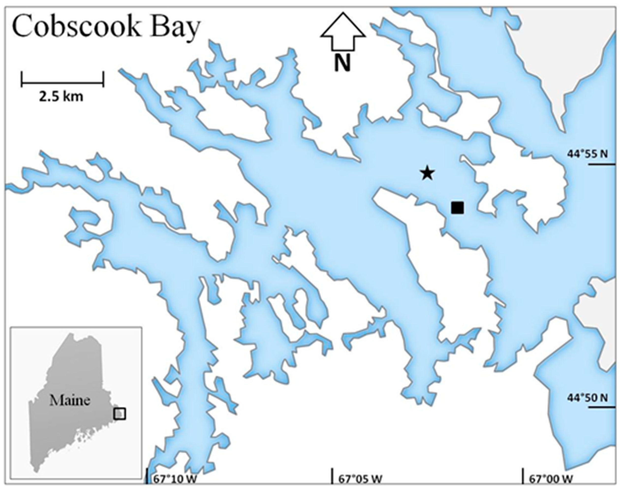
2.1. Data Collection and Study Area

We used a Simrad ES60 echosounder (Horten, Norway) with a single beam Simrad 38/200 Combi W transducer which operated simultaneously at 38 and 200 kHz and had a 31° half-power beam angle. Both frequencies had a pulse duration of 0.512 ms and a ping rate of 2 Hz. Transmit power was 320 W for 38 kHz and 225 W for 200 kHz. The only exception to these collection settings was in March 2011, when the pulse duration was 0.256 ms for both frequencies and transmit power was 200 W for 38 kHz and 225 W for 200 kHz. We calibrated the echosounder annually on a frozen lake prior to that year’s surveys. A frozen lake provided a stable platform that allowed precise placement of copper calibration spheres (60.0 mm for 38 kHz and 13.7 mm for 200 kHz) on the maximum response axis of the acoustic beam. These calibrations were performed for both sets of echosounder settings used during surveys. In-situ on-axis calibrations were performed once every survey during slack tide to ensure consistent system performance.
All data were collected in outer Cobscook Bay (Figure 2) at an “impact” site where the ORPC device was installed (44°54.60′ N, 67°02.74′ W) and at a “control” site 1.6 km seaward (44°54.04′ N, 67°01.71′ W). The transducer was mounted 1.8 m below the water surface on the port side of a 12.2 m boat that was moored at these sites for consecutive 24-hour periods. During each 24-hour survey, the boat changed positions (<100 m) as it swung around its mooring with the change of each tide. The depth at the impact site was approximately 24 m at low tide and 33 m at high tide, and at the control site, depth was approximately 33 m at low tide and 42 m at high tide. The tidal current speeds were similar at both sites, and in fact, the control site was a previously slated site for turbine deployment. Surface current speeds in the area were measured with a flowmeter (Marsh McBirney, Frederick, MD, USA) or Acoustic Doppler Current Profiler (ADCP) (RD Instruments) and were typically less than 2.0 m·s−1 but as fast as 2.5 m·s−1 at maximum flow during a spring tide. In 2011, surface temperature was collected using the transducer’s temperature sensor, and salinity was measured with a hand-held refractometer (Sper Scientific 300011, Sper Scientific, Scottsdale, AZ, USA). In 2012–2013, we deployed a conductivity, temperature, and depth (CTD) sensor (SeaBird Scientific SBE19, SeaBird Scientific, Bellevue, WA, USA) during at least one slack tide per survey for salinity and temperature profiles.
Impact and control sites were surveyed in March, May, June, August, September, and November in 2011, March, May, August, and September 2012 and March 2013. All surveys were scheduled on neap tides to avoid potential confounding effects from lunar tidal harmonics [32]. In each survey, data were collected continuously for 24 h to capture both diel and tidal periodicities [26,32]. There were two exceptions to this: the control site survey in March 2012 was split across two days (29 February and 2 March) because of poor weather. There were no June 2012 data because the impact site was not accessible during preparations for turbine installation, and only 20 h of data were collected for the August 2012 survey due to electronic complications with the echosounder.
The TidGen® BSF was installed prior to the May 2012 survey on 4 April 2012, and the turbine was installed in August 2012, two weeks before that month’s survey. The turbine spanned 6.7–9.5 m above the seafloor. The turbine’s operational state was different for each of the three surveys carried out with the completed device (Table 1). In the August 2012 survey, the turbine was not rotating and thus not generating electricity. The turbine was fully operational (rotating and generating electricity) during the September 2012 survey, except for part of the time during the survey at the control site. In March 2013, the turbine was rotating but not generating electricity (free spinning).

2.2. Data Processing and Analysis
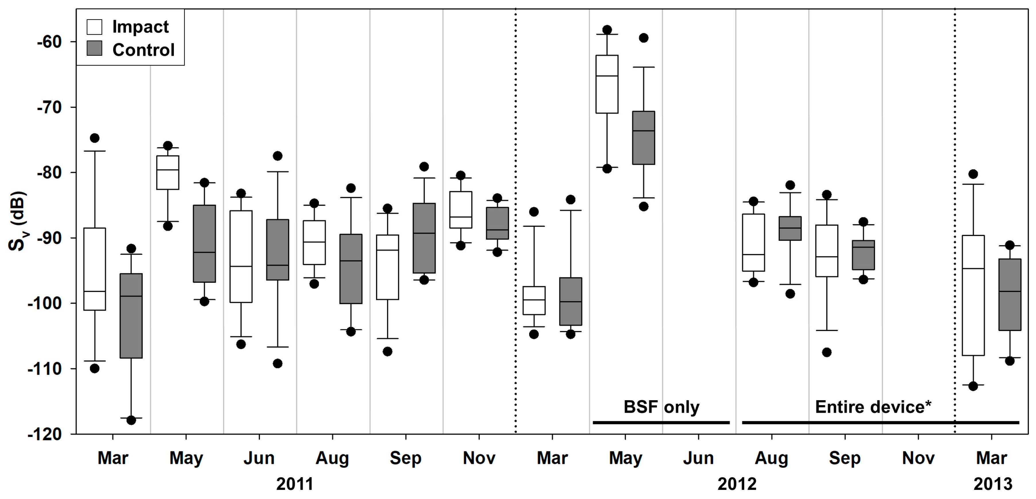
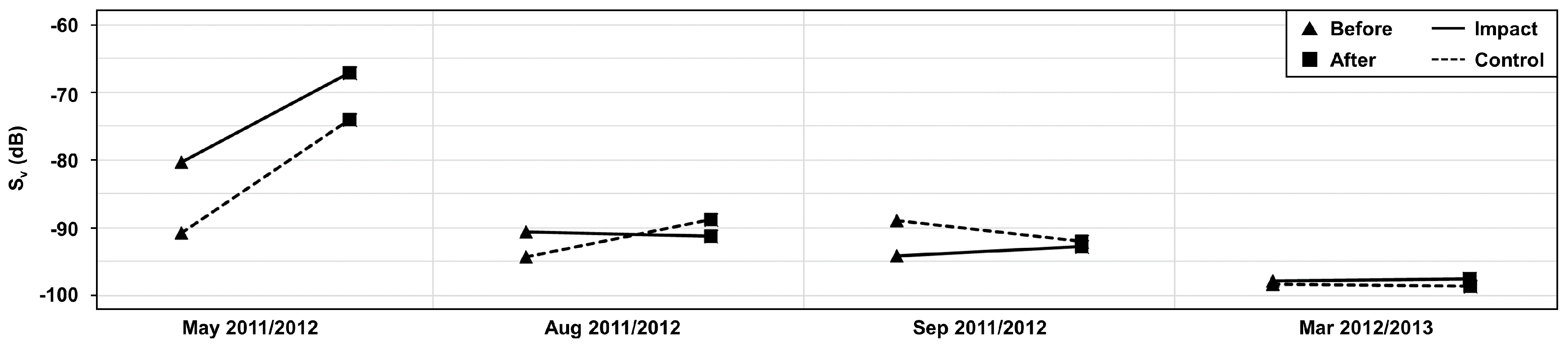
All hydroacoustic data processing was conducted using Echoview® software [38]. Calibration parameters from the winter calibrations were applied to the raw acoustic backscatter data, and sound speed and absorption coefficients were calculated based on water temperature and salinity collected during surveys. A known systematic triangle wave error in data collected with a Simrad ES60 echosounder was investigated and found to be negligible [26]. Using 38 kHz backscatter echograms, a bottom line 0.5 m above bottom was created and smoothed using Echoview® algorithms. Data below this line were excluded from processing.
The data were scrutinized for noise (acoustic signal from non-target sources), which were then removed from analyses. This included entrained air, which often contaminated the upper 10 m of the water column and masked signal from fish. Additionally, data from the bottom 3 m of the water column were removed in May 2011 at both sites due to the presence of a lobster trap and line that remained in the beam for most of the survey. The simultaneous use of ADCPs (one on the boat and one deployed on the seafloor at the impact site) resulted in noise spikes consisting of single contaminated pings in both the 38 and 200 kHz hydroacoustic data. To remove this noise, each ping was compared to those on either side and if the magnitude of the difference between them was above a threshold of 10 dB, the contaminated ping was replaced by interpolating between its adjacent pings [39,40].
The 38 and 200 kHz backscatter data were dB differenced using ∆MVBS analysis [41,42,43,44]. Most data processing methods followed by Korneliusson et al. [45]. The following processing steps were taken for all backscatter data (Sv): (1) data were smoothed and background noise was removed. (2) noise outliers were removed using a series of median filters followed by erosion and dilation filters. (3) a virtual echogram was created using Com_Sv = (Sv 38 kHz + Sv 200 kHz)/2 to find common backscatter between the two frequencies. (4) the 38 kHz mean volume backscattering strength (Sv) was subtracted from the 200 kHz Sv to provide the frequency response, r(f), of the sound scatterers. (5) backscatter was classified based on frequency response categories, where r(f) < 6 dB were fish and r(f) > 6 dB were zooplankton. (6) a mask was created that removed all backscatter from the echogram except for that from fish, as classified in step 5.
Data from running ebb and flood tides, but not slack tides, were analyzed because we were most concerned with fish interactions with a rotating turbine, and the turbine would be static during slack tides. Removing slack tide data also eliminated the possible effects of lengthy detections of the same fish while ensonified in the sound beam for long periods of time, as well as effects of unpredictable boat movements (e.g., swinging about the mooring, along with pitch, roll, and heave which increased when currents were slow). We defined slack tides as the times when the boat was not stable against a taut mooring line, which usually amounted to a time span of 1 hour. Additionally, only data from 0 to 15 m above the seafloor were analyzed to standardize comparisons between the control and impact sites, remove the turbulence in the surface 10 m, and to focus analyses on the depths encompassing the turbine. Ebb and flood tide data were divided into bins that were 2 h wide by 15 m high (except for May 2011 where data from 0–3 m was removed due to fishing equipment interference), measured upward from the seafloor. Two-hour bins were used to ensure that each sample was independent (no autocorrelation at the 5% significance level). Sv, the index of fish density used here, was then calculated and exported from each 2-h bin. Sv is a measure of sound scattered by acoustic targets (in this case, fish) in a unit volume of water, has units of decibels (dB re 1 m−1), and is assumed to be proportional to fish density [27,46].
Statistical analyses were not performed due to small sample sizes and violations of the assumptions of the standard BACI design (primarily confounding factors [36]). Interaction plots of mean Sv values before and after for both the impact and control sites were used to describe possible interaction effects. A possible effect was defined as opposing and crossing slopes of the Sv values of the before/after impact site compared to the before/after control site. Interaction effect size was the difference in mean change in Sv between the two sites.
effect   size   =   ( S v ¯ a f t e r   c o n t r o l   S v ¯ b e f o r e   c o n t r o l )     ( S v ¯ a f t e r   i m p a c t   S v ¯ b e f o r e   i m p a c t )

3. Results

The control and the impact sites had similar trends in relative fish densities, with generally low densities in March and relatively higher in May for all years sampled (Figure 3). At both sites, fish densities were apparently higher in May 2012 than in May 2011, and other months sampled across years did not show such large annual variation (Figure 3).
Median fish density at the impact site was higher than the control site when only the bottom support frame (BSF) was present without the device in May 2012. This same difference was observed prior to the installation of the BSF in May 2011. Overall fish density was higher in May 2012 at both sites than May 2011 (Figure 3), but there was no interaction (Table 1, Figure 4).
Median fish density was higher at the control site than the impact site when the turbine was present but braked (static) in August 2012. Median fish density was lower at the control site compared to the impact site prior to the installation of the turbine and BSF in August 2011 (Figure 3). There was an interaction (slope of the Impact line opposes and crosses the Control line) between the control and impact sites in August 2011 (before) and 2012 (after) the turbine was installed (Table 1, Figure 4). The effect size for this interaction was 6.2 dB.
Median fish density was similar at the control site and impact site when the turbine was present, rotating, and producing power in September 2012 (Figure 3). Median fish density was also similar at the control site than the impact site in September 2011, but with the 90th and 95th percentiles above the range of the impact site. There was no interaction for September sites (impact and control) before and after installation (Table 1, Figure 4).
In the March 2012 survey, prior to BSF and turbine installation, median fish density was similar at the impact site and the control site. After installation, when the device was present and rotating but not generating electricity (2013), median fish density was also similar at the impact site and control site with no interaction (Table 1, Figure 4).

4. Discussion

Fish density at the Cobscook Bay tidal energy site was found to vary noticeably over the course of each year sampled, in agreement with previous work at this site [26,29,32]. While BACI sampling is particularly suited to differentiating the effects of an event from natural variability, and they have been effectively used in previous research on fish and environmental stressors [36,37] we were not able to fully employ the statistical design in this study due to physical difficulties of sampling these habitats resulting in low sample size and confounding effects of (1) the turbine condition changing between sampling periods and (2) apparent response of the fish consistent with behaviors related to ancillary conditions related to the turbine installation (see next paragraph). With these now known confounding effects, this experimental design can be more fully implemented in energetic, dynamic tidal energy sites, where natural spatial and temporal variation in fish presence is high [32].
One of the four paired samples indicated a possible interaction effect of the non-operational MHK device presence on fish density. The only apparent device effect was seen in the August 2011 vs. 2012 comparison, when the turbine was not rotating and was effectively an extension of the BSF. Given the other three comparisons (May, September, and March) indicating no interaction effects of either the BSF alone or of the entire device (in various operational states), the significant difference observed in August was related to something other than turbine operation. One probable explanation is on-water/construction activity occurring at the impact site. The August 2012 survey took place just two weeks after the turbine installation, and there were ongoing vessel and diver activity at that time, both of which previously have been found to affect fish [34,35,47,48]. Separating effects of a known stressor (e.g., an operating turbine) from unquantified stressors (e.g., on-water activities) can prove difficult [49] and result in the inability to apply valid statistical comparisons [36]. While BACI study design does not require all stressors to be measured to detect potential effects of the one in question, it does require unquantified stressors to be similar at both the impact and control sites. Vessel and diver activity are unlikely to be replicated at control sites, so to avoid erroneously attributing changes in fish presence to MHK devices, it is important that future studies attempt to quantify this and other likely stressors as much possible.
Effects of on-water activities on animal presence at marine renewable energy sites have been observed at other locations and suggest construction timing may result in unforeseen indirect effects on additional ecosystem components. Research on juvenile pink salmon (Oncorhynchus gorbuscha) and chum salmon (O. keta) distribution in Puget Sound showed lower fish abundance at a construction site during days of pile driving compared to days without [50]. At offshore wind installations, little tern (Sternula albifrons) [51] studies were used to correlate negative impacts of mono-pile installation on herring spawning success, which created a trophic effect of less forage for little tern chicks. The authors urged precaution of installation timing and associated pile-driving activity. Existing research, along with results presented here, suggests that the effect of construction activities should be separated from the effect of a deployed, operational MHK device, and managed separately.
Fish reactions to a tidal power device may vary based on their encounter with a static (BSF) or dynamic device component. Differences in fish density near the TidGen® turbine were also observed in a separate study that used fish vertical distribution [29], and smaller horizontal bin size (30 min). The vertical distribution of fish in that study was significantly different after device installation in the same August comparison as well. Shen et al. [16] used fish vertical distributions and other hydroacoustic data to model the probability of fish encountering the deployed TidGen® MHK device. They determined the probability of fish upstream of the device encountering the entire device (BSF and turbine, 0–9.5 m above the bottom) was approximately 50%, and the probability encountering just the turbine (6.7–9.5 m above the bottom) was approximately 6%, depending on diel conditions (night or day). If only those fish at the depth of the turbine (~6% of the water column total Sv) modify their behavior (e.g., in response to dynamic device component) by vertical [29] or horizontal movement, it is likely that the change in water column density or vertical distribution would be difficult to observe and statistically insignificant. However, if fish encountering the entire device (~50% of the water column total Sv) change their behavior (in response to both the dynamic and static device components), the change would be more evident since more fish are moving. As such, the interaction observed in the August data from this study and Staines et al. [29] may reflect fish changing their distribution elsewhere in the water column, not just at the depth of the dynamic turbine component of the TidGen® device. It may be necessary to determine if the mechanisms resulting in behavior change are a response to a device is related to its dynamic parts only, the static components or both. This will be important since behavioral changes have the potential to affect fish immigration and emigration through these high energy areas targeted for tidal power devices, potentially influencing larger-scale population responses to this anthropogenic influence.
The index of fish density used in this work was mean volume backscattering strength (Sv) of the lower 15 m of the water column, from data obtained with a single beam echosounder. Other research applications using down-looking hydroacoustics scale backscatter with target strength information provided by split-beam transducers or apply statistical deconvolution techniques to scale backscatter with fish size for density or abundance estimates [27,52,53]. Their goals were different from those of this study and the scaling of Sv with TS can introduce bias that using unscaled Sv does not. We chose not to attempt to scale Sv in these ways, as our goal was not to separate species by target strength or create absolute fish density estimates. Instead, we wanted to generate an index of fish presence at the project and control sites as a baseline assessment. Single-beam echosounders are less expensive than split-beam models and were financially ideal for early-stage monitoring efforts. The use of dual-frequency (38 and 200 kHz) hydroacoustics enabled the application of dB differencing processing methods that removed the majority of unwanted zooplankton backscatter from that of fish, resulting in a good density index of fishes that may be exposed to the MHK device at the times surveyed. This index is a composite suite of the mixed fish assemblage present in Cobscook Bay [22].
The changes in fish density around a single deployed device are unlikely to be representative of a larger disturbance in the form of operational, commercial-scale arrays. A single device presents little in the way of an obstacle when compared to the entire cross-sectional area of a tidal channel like outer Cobscook Bay. However, the probability that multiple devices will disrupt movement, whether small-scale daily excursions or large-scale migrations, is yet to be tested and will present a new set of challenges for separating the effects of environmental variables from those of an MHK device array. Similar challenges have been associated with birds and bats around wind turbines. Doty and Martin [54] studied a single pilot turbine for one year in South Africa and noted 18 bat casualties and 1 bird casualty. Like our study, they referenced a single pilot device and showed an effect on bats and birds. However, a single operational device is difficult to scale-up to several devices or an array. Associated scaling of monitoring to capture differences between single devices and arrays is developing, as there are also studies referencing large-scale arrays that also find bat and bird mortality [55]. The array studies did not develop from single device studies and without the early, single-device monitoring, it is difficult to say how effects differ with the increasing number of devices. Monitoring should begin as early as possible in the research and development stage for any new technology, and this should include single pilot device research. The referenced bird and bat studies, along with this research, show that as renewable energy industries move forward, it will be important to continue research on fish behavior around deployed devices during installation and deployment. Effects and potential impacts could change such as large-scale ecosystem cascades from lack of forage fish for piscivorous species [56]. Early-stage, single-device monitoring can provide preliminary data on potential effects of devices on fish and provide the basis for array-stage research questions and sampling methods to answer them.

5. Conclusions

Effects of installing an MHK device on fish density in its surrounding tidally dynamic area were demonstrated here. While this, along with other factors, confounded the full implementation of a BACI design, valuable information was gained that should influence future monitoring activities at MHK sites. The impact of these effects on the fish assemblage in the region is yet unknown. Other construction-related disturbances in the area in combination with the TidGen® deployment may explain the observed fish density difference. Device installation, maintenance, and decommissioning will likely prove to be times of highest disturbance around MHK devices [57]. It will be important to time such activities to avoid major fish migrations or presence of endangered and threatened species. Insight from this research has aided permitting for local and regional regulatory bodies, industry, and local stakeholders to make decisions regarding the social and legal acceptance of tidal power development and future device deployments [6]. Continued research is needed in the area of fish monitoring, along with other environmental assessments (e.g., mammals, birds, underwater noise), to allow this renewable energy source to develop into a sustainable, commercially viable market to further enable carbon emission mitigation of climate change effects.

Author Contributions

Conceptualization, G.Z., H.V., and G.S.; methodology, H.V., G.Z., and G.S.; validation, G.S., H.V., and G.Z.; formal analysis, G.S., H.V., and G.Z.; investigation, G.Z., H.V., and G.S.; resources, G.Z.; data curation, H.V. and G.S.; writing—original draft preparation, G.S.; writing—review and editing, G.Z. and H.V.; visualization, H.V. and G.S.; supervision, G.Z.; project administration, G.Z.; funding acquisition, G.Z. and H.V.

Funding

The US Department of Energy supported this research [grant numbers: DE-EE0003266, DE-EE0003647, DE-EE0006384]. This project was supported by the USDA National institute of Food and Agriculture, Hatch Project Number ME0-031716 through the Maine Agricultural & Forest Experiment Station. Maine Agricultural and Forest Experiment Station Publication Number 3709.

Acknowledgments

We thank Ocean Renewable Power Company for contributing resources and their cooperation to make this research possible. Captain George Harris Jr. and crew aided with all boat work. Thanks to the Maine Tidal Power Initiative at the University of Maine for their contributions. The views expressed herein are those of the authors and do not necessarily reflect the views of Ocean Renewable Power Company or any of its sub agencies.

Conflicts of Interest

G.S., H.V., and G.Z. declare no conflict of interest. Authors must identify and declare any personal circumstances or interest that may be perceived as inappropriately influencing the representation or interpretation of reported research results. The funder had no role in the design of the study; in the collection, analyses, or interpretation of data; in the writing of the manuscript, or in the decision to publish the results.

References

  1. Li, Y.; Willman, L. Feasibility analysis of offshore renewables penetrating local energy systems in remote oceanic areas–a case study of emissions from an electricity system with tidal power in Southern Alaska. Appl. Energy 2014, 117, 42–53. [Google Scholar] [CrossRef]
  2. Roberts, A.; Thomas, B.; Sewell, P.; Khan, Z.; Balmain, S.; Gillman, J. Current tidal power technologies and their suitability for applications in coastal and Marine areas. J. Ocean Eng. Mar. Energy 2016, 2, 227–245. [Google Scholar] [CrossRef]
  3. Zhou, Z.; Benbouzid, M.; Charpentier, J.-F.; Scuiller, F.; Tang, T. Developments in large marine current turbine technologies–A review. Renew. Sustain. Energy Rev. 2017, 71, 852–858. [Google Scholar] [CrossRef]
  4. Copping, A.; Sather, N.; Hanna, L.; Whiting, J.; Zydlewski, G.; Staines, G.; Gill, A.; Hutchison, I.; O′Hagan, A.; Simas, T. Annex IV 2016 State of the Science Report: Environmental effects of Marine renewable energy development around the world. Available online: https://tethys.pnnl.gov/publications/state-of-the-science-2016 Ocean Energy Systems (accessed on 8 October 2019).
  5. Tethys. Available online: http://www.tethys.pnnl.gov (accessed on 8 October 2019).
  6. Jansujwicz, J.S.; Johnson, T.R. The Maine Tidal Power Initiative: Transdisciplinary Sustainability Science Research for the responsible development of tidal power. Sustain. Sci. 2015, 10, 75–86. [Google Scholar] [CrossRef]
  7. Gregory, R.; Ohlson, D.; Arvai, J. Deconstructing adaptive Management: Criteria for applications to environmental Management. Ecol. Appl. 2006, 16, 2411–2425. [Google Scholar] [CrossRef]
  8. Forward, R.B.; Tankersley, R.A. Selective tidal-stream transport of Marine animals. Ocean Mar. Biol. 2001, 39, 305–353. [Google Scholar]
  9. Shields, M.; Ford, A.; Woolf, D. Ecological considerations for tidal energy development in Scotland. In Proceedings of the 10th World Renewable Energy Conference, Glasgow, Scotland, 19–25 July 2008. [Google Scholar]
  10. Boehlert, G.W.; Gill, A.B. Environmental and ecological effects of ocean renewable energy development: A current synthesis. Oceanography 2010, 23, 68–81. [Google Scholar] [CrossRef]
  11. Hammar, L.; Andersson, S.; Eggertsen, L.; Haglund, J.; Gullström, M.; Ehnberg, J.; Molander, S. Hydrokinetic turbine effects on fish swimming behaviour. PLoS ONE 2013, 8, e84141. [Google Scholar] [CrossRef]
  12. Broadhurst, M.; Barr, S.; Orme, C.D.L. In-situ ecological interactions with a deployed tidal energy device; an observational pilot study. Ocean Coast. Manag. 2014, 99, 31–38. [Google Scholar] [CrossRef]
  13. Viehman, H.A.; Zydlewski, G.B. Fish interactions with a commercial-scale tidal energy device in the natural environment. Estuaries Coasts 2015, 38, 241–252. [Google Scholar] [CrossRef]
  14. Stokesbury, M.J.; Logan-Chesney, L.M.; McLean, M.F.; Buhariwalla, C.F.; Redden, A.M.; Beardsall, J.W.; Broome, J.E.; Dadswell, M.J. Atlantic sturgeon spatial and temporal distribution in Minas Passage, Nova Scotia, Canada, a region of future tidal energy extraction. PLoS ONE 2016, 11, e0158387. [Google Scholar] [CrossRef] [PubMed]
  15. Bevelhimer, M.; Scherelis, C.; Colby, J.; Adonizio, M.A. Hydroacoustic assessment of behavioral responses by fish passing near an operating tidal turbine in the east river, New York. Trans. Am. Fish. Soc. 2017, 146, 1028–1042. [Google Scholar] [CrossRef]
  16. Shen, H.; Zydlewski, G.B.; Viehman, H.A.; Staines, G. Estimating the probability of fish encountering a marine hydrokinetic device. Renew. Energy 2016, 97, 746–756. [Google Scholar] [CrossRef] [Green Version]
  17. Fraser, S.; Williamson, B.J.; Nikora, V.; Scott, B.E. Fish distributions in a tidal channel indicate the behavioural impact of a Marine renewable energy installation. Energy Rep. 2018, 4, 65–69. [Google Scholar] [CrossRef]
  18. Wiesebron, L.E.; Horne, J.K.; Scott, B.E.; Williamson, B.J. Comparing nekton distributions at two tidal energy sites suggests potential for generic environmental monitoring. Int. J. Mar. Energy 2016, 16, 235–249. [Google Scholar] [CrossRef] [Green Version]
  19. Copping, A.; Battey, H.; Brown-Saracino, J.; Massaua, M.; Smith, C. An international assessment of the environmental effects of Mar. energy development. Ocean Coast. Manag. 2014, 99, 3–13. [Google Scholar] [CrossRef]
  20. Trump, C.L.; Leggett, W.C. Optimum swimming speeds in fish: The problem of currents. Can. J. Fish. Aquat. Sci. 1980, 37, 1086–1092. [Google Scholar] [CrossRef]
  21. Weihs, D. Tidal stream transport as an efficient method for migration. ICES J. Mar. Sci. 1978, 38, 92–99. [Google Scholar] [CrossRef]
  22. Vieser, J.D. Collaborative Research on Finfish, Their Distribution, and Diversity in Cobscook Bay, Maine. Master′s Thesis, University of Maine, Orono, ME, USA, 2014. [Google Scholar]
  23. Redden, A.M.; Broome, J.; Keyser, F.; Stokesbury, M.; Bradford, R.; Gibson, J.; Halfyard, E. Use of animal tracking technology to assess potential risks of tidal turbine interaction with fish. In Proceedings of the 2nd International Conference on Environmental Interactions of Mar. Renewable Energy Technologies (EIMR2014), Outer Hebrides, Scotland, 28 April–2 May 2014. [Google Scholar]
  24. Keyser, F.M.; Broome, J.E.; Bradford, R.G.; Sanderson, B.; Redden, A.M. Winter presence and temperature-related diel vertical migration of striped bass (Morone saxatilis) in an extreme high-flow passage in the inner Bay of Fundy. Can. J. Fish. Aquat. Sci. 2016, 73, 1777–1786. [Google Scholar] [CrossRef]
  25. Broome, J.E.; Redden, A.M.; Keyser, F.M.; Stokesbury, M.J.W.; Bradford, R.G. Passive acoustic telemetry detection of Striped Bass at the FORCE TISEC test site in Minas Passage, Nova Scotia, Canada. In Proceedings of the 3rd Mar. Energy Technology Symposium, Washington, DC, USA, 27–29 April 2015; pp. 1–5. [Google Scholar]
  26. Viehman, H.A.; Zydlewski, G.B.; McCleave, J.D.; Staines, G.J. Using hydroacoustics to understand fish presence and vertical distribution in a tidally dynamic region targeted for energy extraction. Estuaries Coasts 2015, 38, 215–226. [Google Scholar] [CrossRef]
  27. Simmonds, J.; MacLennan, D.N. Fisheries Acoustics: Theory and Practice; John Wiley & Sons: Hoboken, NJ, USA, 2008; ISBN 0-470-99529-7. [Google Scholar]
  28. Urmy, S.S.; Horne, J.K.; Barbee, D.H. Measuring the vertical distributional variability of pelagic fauna in Monterey Bay. ICES J. Mar. Sci. 2012, 69, 184–196. [Google Scholar] [CrossRef] [Green Version]
  29. Staines, G.; Zydlewski, G.; Viehman, H.; Shen, H.; McCleave, J. Changes in vertical fish distributions near a hydrokinetic device in Cobscook Bay, Maine, USA. In Proceedings of the 11th European Wave and Tidal Energy Conference (EWTEC2015), Nantes, France, 6–11 September 2015; pp. 6–11. [Google Scholar]
  30. Matveev, V.F.; Steven, A.D.L. The effects of salinity, turbidity and flow on fish biomass estimated acoustically in two tidal rivers. Mar. Freshw. Res. 2014, 65, 267–274. [Google Scholar] [CrossRef]
  31. Park, J.M.; Huh, S.-H.; Baeck, G.W. Temporal variations of fish assemblage in the surf zone of the Nakdong River Estuary, southeastern Korea. Anim. Cells Syst. 2015, 19, 350–358. [Google Scholar] [CrossRef] [Green Version]
  32. Viehman, H.A.; Zydlewski, G.B. Multi-scale temporal patterns in fish presence in a high-velocity tidal channel. PLoS ONE 2017, 12, e0176405. [Google Scholar] [CrossRef]
  33. Stanley, D.R.; Wilson, C.A. Seasonal and spatial variation in the abundance and size distribution of fishes associated with a petroleum platform in the northern Gulf of Mexico. Can. J. Fish. Aquat. Sci. 1997, 54, 1166–1176. [Google Scholar]
  34. Handegard, N.O.; Michalsen, K.; Tjøstheim, D. Avoidance behaviour in cod (Gadus morhua) to a bottom-trawling vessel. Aquat. Living Resour. 2003, 16, 265–270. [Google Scholar] [CrossRef]
  35. Draštík, V.; Kubečka, J. Fish avoidance of acoustic survey boat in shallow waters. Fish. Res. 2005, 72, 219–228. [Google Scholar] [CrossRef]
  36. Smith, E.P.; Orvos, D.R.; Cairns Jr, J. Impact assessment using the before-after-control-impact (BACI) model: Concerns and comments. Can. J. Fish. Aquat. Sci. 1993, 50, 627–637. [Google Scholar] [CrossRef]
  37. Marks, J.C.; Haden, G.A.; O′Neill, M.; Pace, C. Effects of flow restoration and exotic species removal on recovery of native fish: Lessons from a dam decommissioning. Restor. Ecol. 2010, 18, 934–943. [Google Scholar] [CrossRef]
  38. Echoview Software, Version 8.0.; Echoview Software Pty Ltd.: Hobart, Australia, 2015.
  39. Anderson, C.I.H.; Brierley, A.S.; Armstrong, F. Spatio-temporal variability in the distribution of epi-and meso-pelagic acoustic backscatter in the Irminger Sea, North Atlantic, with implications for predation on Calanus finmarchicus. Mar. Biol. 2005, 146, 1177–1188. [Google Scholar] [CrossRef]
  40. Ryan, T.E.; Downie, R.A.; Kloser, R.J.; Keith, G. Reducing bias due to noise and attenuation in open-ocean echo integration data. ICES J. Mar. Sci. 2015, 72, 2482–2493. [Google Scholar] [CrossRef] [Green Version]
  41. Madureira, L.S.; Everson, I.; Murphy, E.J. Interpretation of acoustic data at two frequencies to discriminate between Antarctic krill (Euphausia superba Dana) and other scatterers. J. Plankton Res. 1993, 15, 787–802. [Google Scholar] [CrossRef]
  42. Kang, M.; Furusawa, M.; Miyashita, K. Effective and accurate use of difference in mean volume backscattering strength to identify fish and plankton. ICES J. Mar. Sci. 2002, 59, 794–804. [Google Scholar] [CrossRef] [Green Version]
  43. Korneliussen, R.J.; Ona, E. An operational system for processing and visualizing multi-frequency acoustic data. ICES J. Mar. Sci. 2002, 59, 293–313. [Google Scholar] [CrossRef] [Green Version]
  44. Korneliussen, R.J.; Ona, E. Verified Acoustic Identification of Atlantic Mackerel; ICES: Sale, UK, 2004. [Google Scholar]
  45. Korneliussen, R.J.; Heggelund, Y.; Eliassen, I.K.; Johansen, G.O. Acoustic species identification of schooling fish. ICES J. Mar. Sci. 2009, 66, 1111–1118. [Google Scholar] [CrossRef] [Green Version]
  46. Foote, K.G. Linearity of fisheries acoustics, with addition theorems. J. Acoust. Soc. Am. 1983, 73, 1932–1940. [Google Scholar] [CrossRef]
  47. Misund, O.A. Sonar Observations of Schooling Herring: School Dimensions, Swimming Behaviour, and Avoidance of Vessel and Purse Seine; ICES: Sale, UK, 1990. [Google Scholar]
  48. Stanley, D.R.; Wilson, C.A. Effect of scuba divers on fish density and target strength estimates from stationary dual-beam hydroacoustics. Trans. Am. Fish. Soc. 1995, 124, 946–949. [Google Scholar] [CrossRef]
  49. Crain, C.M.; Kroeker, K.; Halpern, B.S. Interactive and cumulative effects of multiple human stressors in Mar. systems. Ecol. Lett. 2008, 11, 1304–1315. [Google Scholar] [CrossRef]
  50. Feist, B.E.; Anderson, J.J.; Miyamoto, R. Potential impacts of pile driving on juvenile pink (Oncorhynchus gorbuscha) and chum (O. keta) salmon behavior and distribution; University of Washington: Seattle, WA, USA, 1991. [Google Scholar]
  51. Perrow, M.R.; Gilroy, J.J.; Skeate, E.R.; Tomlinson, M.L. Effects of the construction of Scroby Sands offshore wind farm on the prey base of Little tern Sternula albifrons at its most important UK colony. Mar. Pollut. Bull. 2011, 62, 1661–1670. [Google Scholar] [CrossRef]
  52. Rudstam, L.G.; Lindem, T.; Hansson, S. Density and in situ target strength of herring and sprat: A comparison between two methods of analyzing single-beam sonar data. Fish. Res. 1988, 6, 305–315. [Google Scholar] [CrossRef]
  53. Gurshin, C.W.; Howell, W.H.; Jech, J.M. Synoptic acoustic and trawl surveys of spring-spawning Atlantic cod in the Gulf of Maine cod spawning protection area. Fish. Res. 2013, 141, 44–61. [Google Scholar] [CrossRef]
  54. Doty, A.C.; Martin, A.P. Assessment of bat and avian mortality at a pilot wind turbine at Coega, Port Elizabeth, Eastern Cape, South Africa. N. Z. J. Zool. 2013, 40, 75–80. [Google Scholar] [CrossRef] [Green Version]
  55. Kuvlesky Jr, W.P.; Brennan, L.A.; Morrison, M.L.; Boydston, K.K.; Ballard, B.M.; Bryant, F.C. Wind energy development and wildlife conservation: Challenges and opportunities. J. Wildl. Manag. 2007, 71, 2487–2498. [Google Scholar] [CrossRef]
  56. Neill, S.M.; Ylitalo, G.M.; West, J.E. Energy content of Pacific salmon as prey of northern and southern resident killer whales. Endanger. Species Res. 2014, 25, 265–281. [Google Scholar] [Green Version]
  57. Gill, A.B. Offshore renewable energy: Ecological implications of generating electricity in the coastal zone. J. Appl. Ecol. 2005, 42, 605–615. [Google Scholar] [CrossRef]
Figure 1. Illustration of Ocean Renewable Power Company’s TidGen® Power System with turbine and bottom support frame (length 31.2 m, width: 15.2 m, height 9.5 m).
Sustainability 11 06262 g001
Figure 2. Map of Cobscook Bay, Maine. The star indicates the location of the impact site and the square indicates the location of the control site.
Sustainability 11 06262 g002
Figure 3. Box-and-whisker plots to describe fish density index, Sv, from 0–15 m above the seafloor for each 24-hour survey of control and impact sites from 2011–2013 in Cobscook Bay, Maine. Boxes indicate the 25th, 50th, and 75th percentiles within each group. The whiskers represent the 10th and 90th percentiles, while the dots represent the 5th and 95th percentiles. The percentiles, whiskers, and dots indicate the spread of the fish density indices obtained during each survey. The impact site is the white box of each pair and the control site is gray. See Table 1 for details on turbine operational state during each “after” survey at the impact site.
Sustainability 11 06262 g003
Figure 4. Interaction plot showing before, after, impact, and control pairings. The x-axis indicates the month and year of compared surveys. The y-axis is mean volume backscatter, Sv (dB re 1 m−1). The impact site is represented by the solid line and the control site by the dashed line. Points indicate mean water column Sv for each 24-hour survey. Surveys taking place before and after device installation are represented by triangles and squares, respectively.
Sustainability 11 06262 g004
Table 1. Comparisons of mean volume backscattering strength (Sv) data collected at impact and control sites before and after the TidGen® was installed, with device operational status.
MonthBefore Device InstallationAfter Device InstallationDevice Status in “After” Survey
May20112012BSF present
Turbine absent
Not generating
August20112012Turbine present
Not rotating
Not generating
September20112012Turbine present
Rotating
generating
March20122013Turbine present
Rotating
Not generating

