New Perspectives for Mapping Global Population Distribution Using World Settlement Footprint Products

 ,
,  , , , , and
Abstract
1. Introduction
2. Materials and Methods
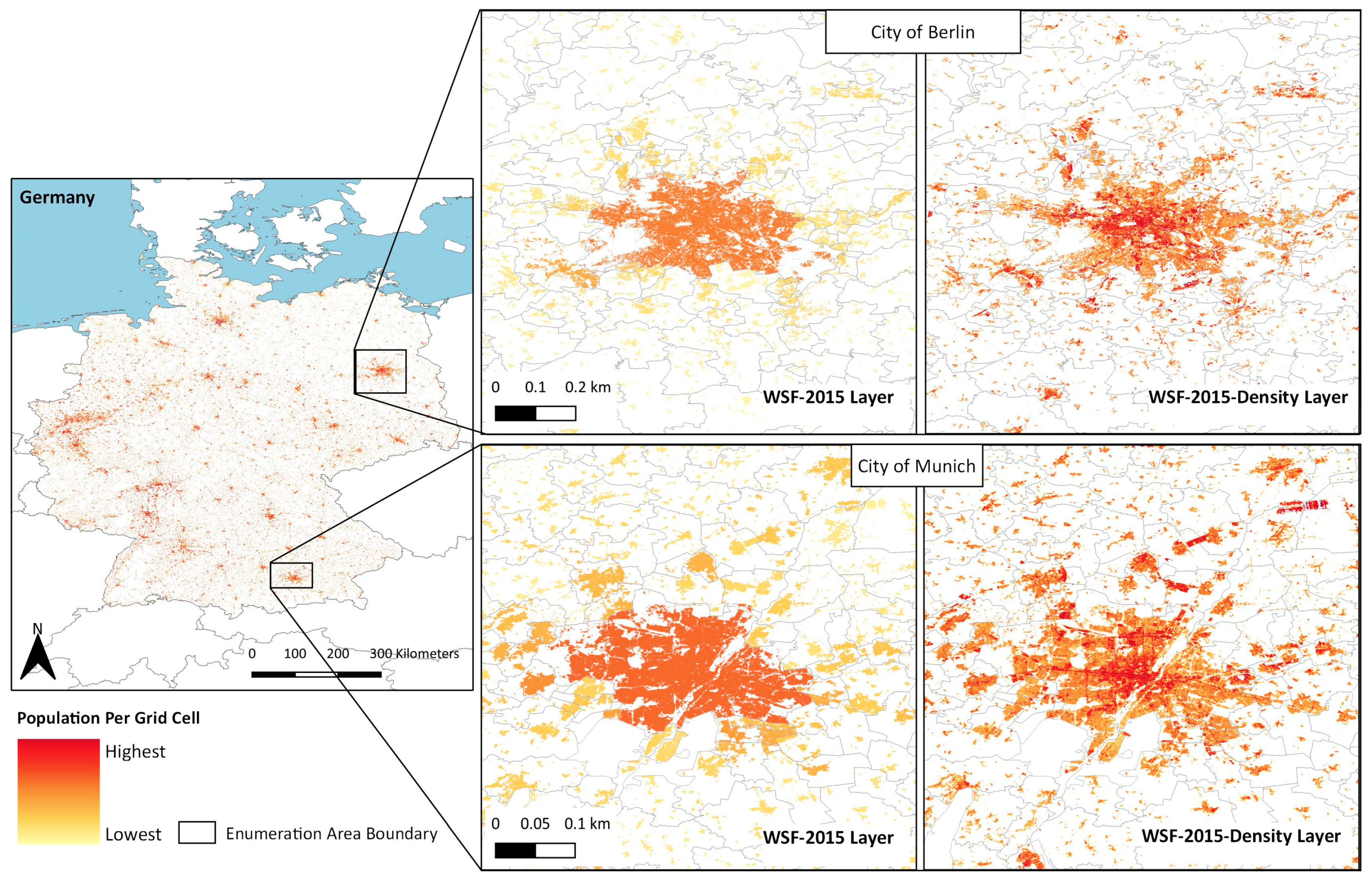
2.1. Input Geospatial Covariates: WSF-2015 and WSF-2015-Density Layers
2.1.1. WSF-2015 Layer
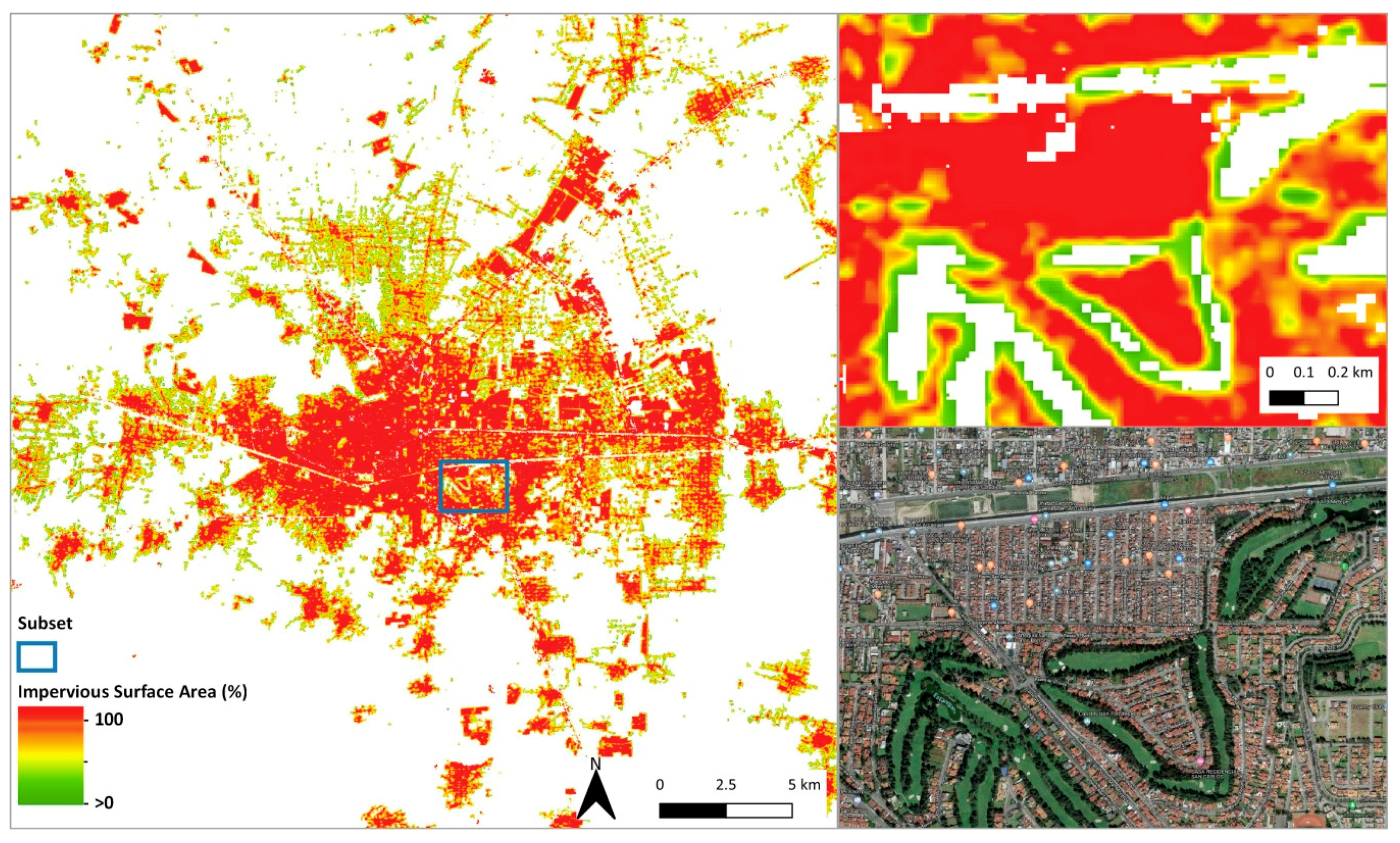
2.1.2. WSF-2015-Density Layer
2.2. Input Census Data
2.3. Population Distribution: Dasymetric Mapping Approach
2.4. Quantitative Accuracy Assessment
3. Results
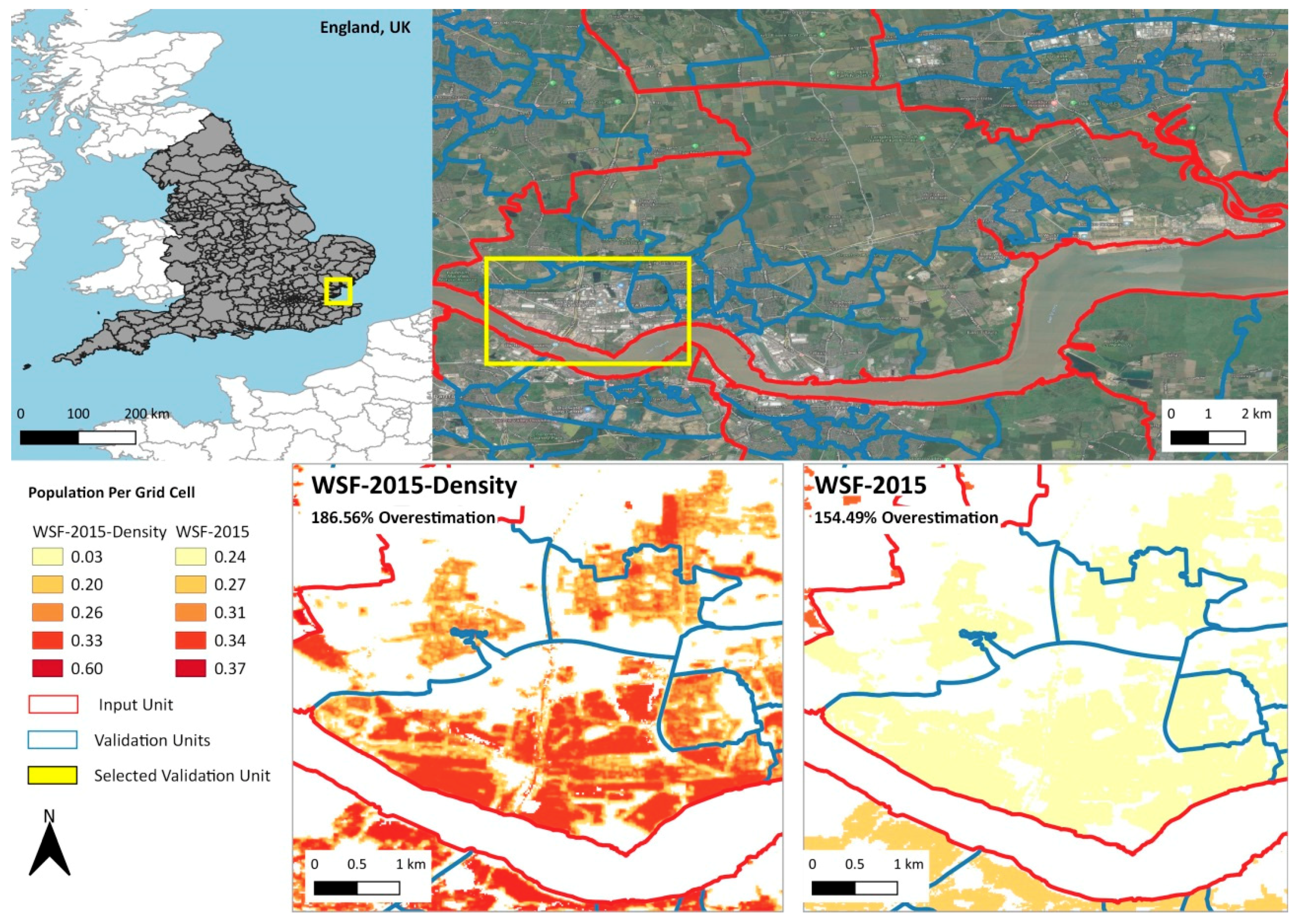
3.1. Visual Assessment of the Population Distribution Maps
3.2. Accuracy Assessment
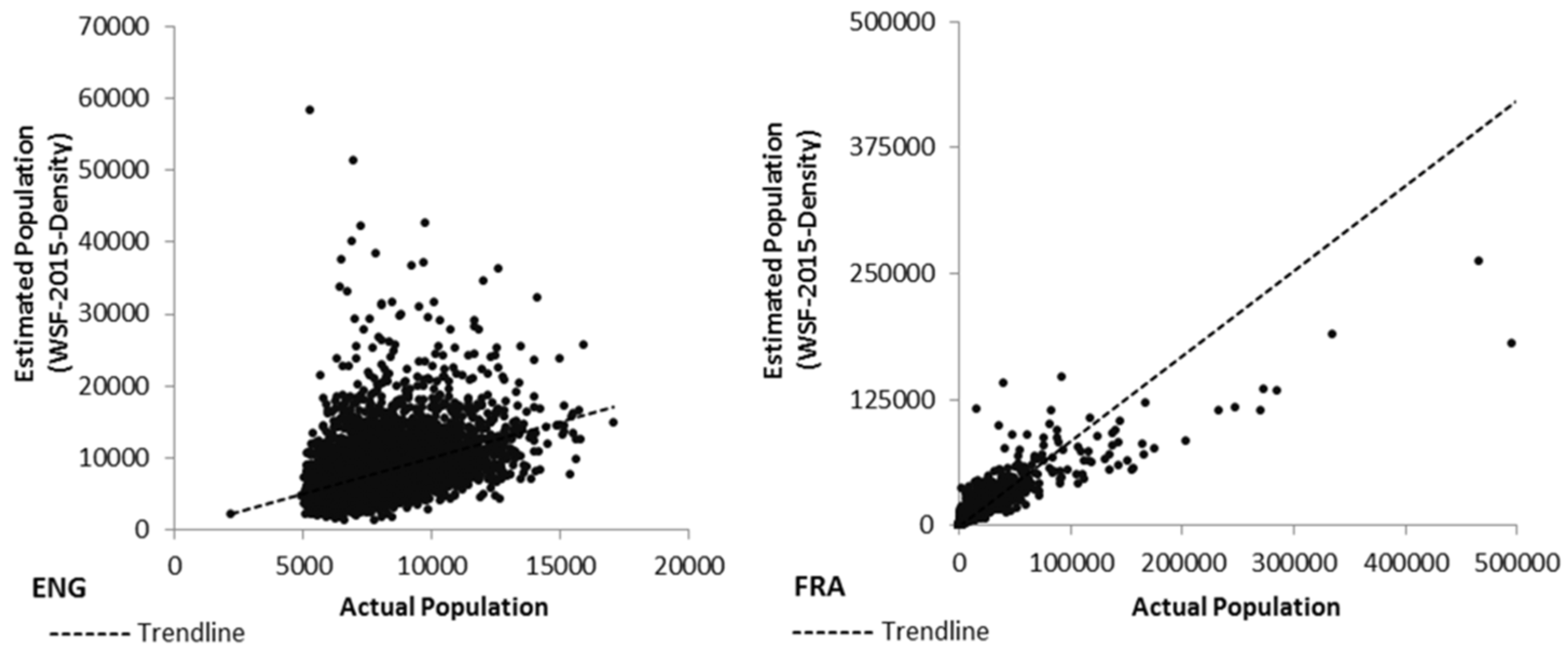
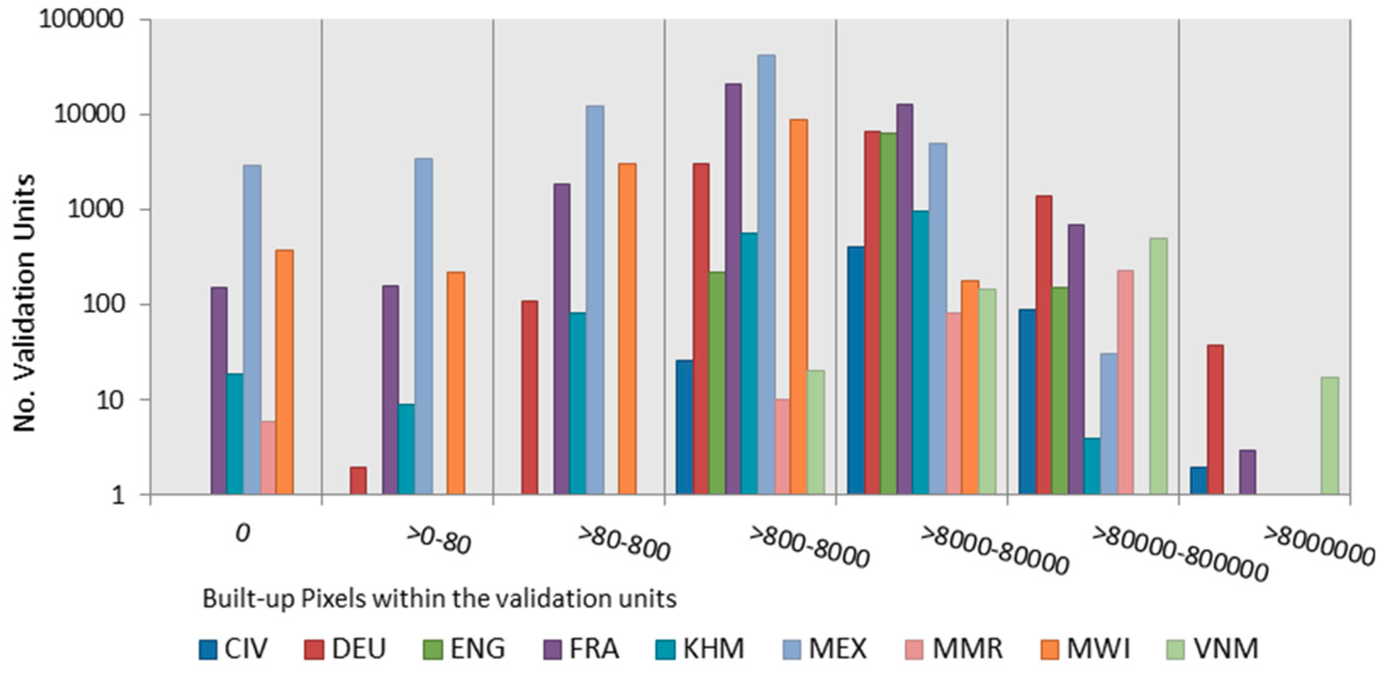
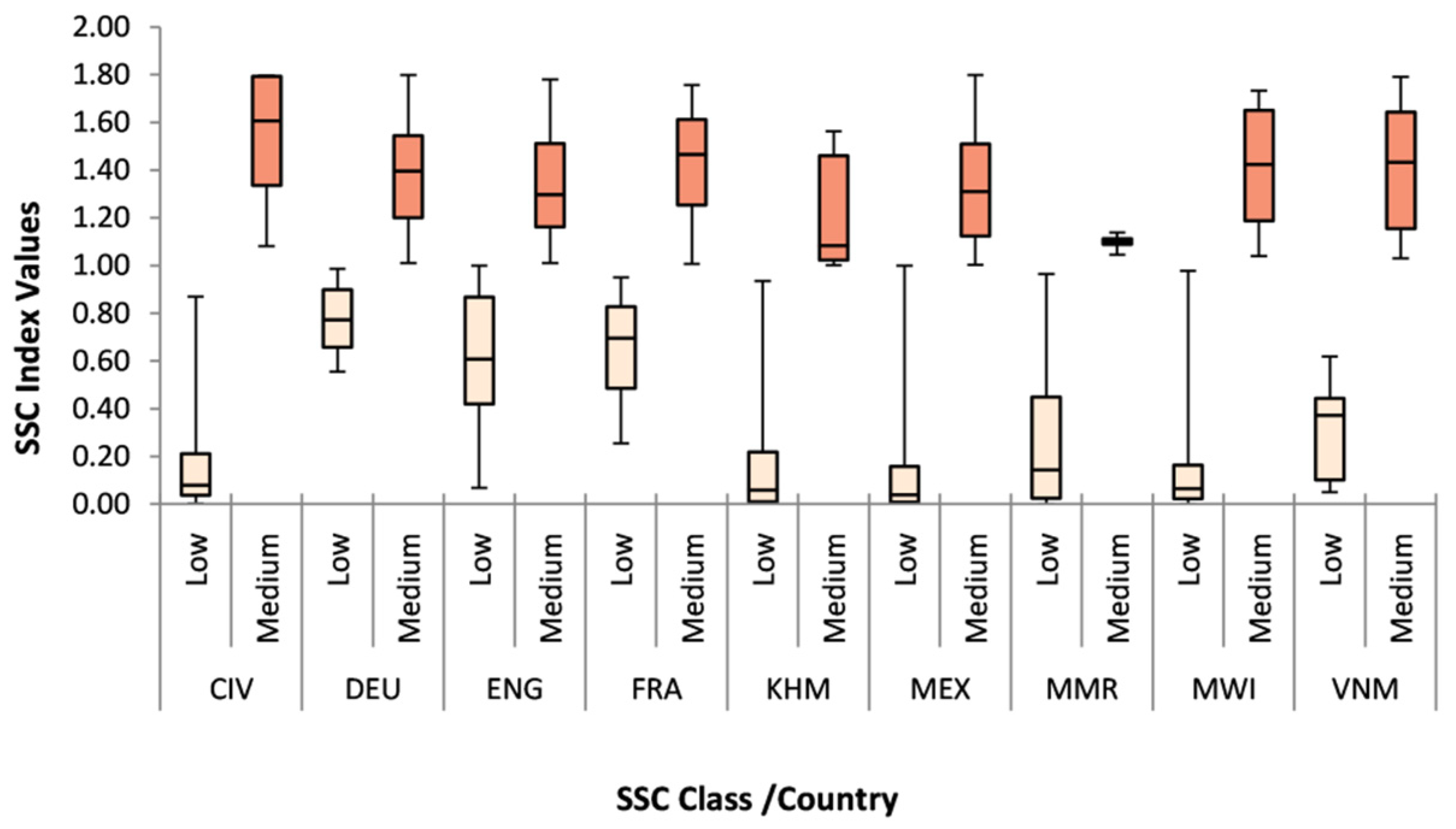
3.2.1. Analyses at the Validation Unit Level
3.2.2. Analyses at the Input Unit Level
4. Discussion
5. Conclusions
Author Contributions
Funding
Acknowledgments
Conflicts of Interest
References
- United Nations. World Population Prospects 2019: Ten Key Findings; United Nations, Department of Econimic and Social Affairs, Population Division: New York, NY, USA, 2019. [Google Scholar]
- United Nations. World Population Prospects 2019: Highlights.ST/ESA/SER.A/423; United Nations, Department of Econimic and Social Affairs, Population Division: New York, NY, USA, 2019. [Google Scholar]
- Balk, D.L.; Deichmann, U.; Yetman, G.; Pozzi, F.; Hay, S.I.; Nelson, A. Determining Global Population Distribution: Methods, Applications and Data. Adv. Parasitol. 2006, 62, 119–156. [Google Scholar] [PubMed]
- Nieves, J.J.; Stevens, F.R.; Gaughan, A.E.; Linard, C.; Sorichetta, A.; Hornby, G.; Patel, N.N.; Tatem, A.J. Examining the correlates and drivers of human population distributions across low- and middle-income countries. J. R. Soc. Interface 2017, 14, 20170401. [Google Scholar] [CrossRef] [PubMed]
- Center for International Earth Science Information Network - CIESIN - Columbia University; International Food Policy Research Institute - IFPRI; The World Bank; Centro Internacional de Agricultura Tropical - CIAT. Global Rural-Urban Mapping Project, Version 1 (GRUMPv1): Population Density Grid; NASA Socioeconomic Data and Applications Center (SEDAC): Palisades, NY, USA, 2011.
- Doxsey-Whitfield, E.; MacManus, K.; Adamo, S.B.; Pistolesi, L.; Squires, J.; Borkovska, O.; Baptista, S.R. Taking Advantage of the Improved Availability of Census Data: A First Look at the Gridded Population of the World, Version 4. Papers Appl. Geogr. 2015, 1, 226–234. [Google Scholar] [CrossRef]
- Center for International Earth Science Information Network - CIESIN - Columbia University. Gridded Population of the World, Version 4 (GPWv4): Population Count Adjusted to Match 2015 Revision of UN WPP Country Totals, Revision 11; NASA Socioeconomic Data and Applications Center (SEDAC): Palisades, NY, USA, 2018.
- Dobson, J.E.; Bright, E.A.; Coleman, P.R.; Durfee, R.C.; Worley, B.A. LandScan: a global population database for estimating populations at risk. Photogramm. Eng. Remote Sens. 2000, 66, 849–857. [Google Scholar]
- Bhaduri, B.; Bright, E.; Coleman, P.; Urban, M.L. LandScan USA: a high-resolution geospatial and temporal modeling approach for population distribution and dynamics. GeoJournal 2007, 69, 103–117. [Google Scholar] [CrossRef]
- Freire, S.; Doxsey-Whitfield, E.; MacManus, K.; Mills, J.; Pesaresi, M. Development of new open and free multi-temporal global population grids at 250 m resolution. In Proceedings of the AGILE, Helsinki, Finland, 14–17 June 2016. [Google Scholar]
- Freire, S.; Kemper, T.; Pesaresi, M.; Florczyk, A.; Syrris, V. Combining GHSL and GPW to improve global population mapping. In Proceedings of the 2015 IEEE International Geoscience and Remote Sensing Symposium (IGARSS), Milan, Italy, 26–31 July 2015; pp. 2541–2543. [Google Scholar]
- Lloyd, C.T.; Sorichetta, A.; Tatem, A.J. High resolution global gridded data for use in population studies. Sci. Data 2017, 4, 170001. [Google Scholar] [CrossRef]
- Stevens, F.R.; Gaughan, A.E.; Linard, C.; Tatem, A.J. Disaggregating census data for population mapping using random forests with remotely-sensed and ancillary data. PLoS ONE 2015, 10, e0107042. [Google Scholar] [CrossRef]
- Sorichetta, A.; Hornby, G.M.; Stevens, F.R.; Gaughan, A.E.; Linard, C.; Tatem, A.J. High-resolution gridded population datasets for Latin America and the Caribbean in 2010, 2015, and 2020. Sci. Data 2015, 2, 150045. [Google Scholar] [CrossRef]
- Gaughan, A.E.; Stevens, F.R.; Huang, Z.; Nieves, J.J.; Sorichetta, A.; Lai, S.; Ye, X.; Linard, C.; Hornby, G.M.; Hay, S.I.; et al. Spatiotemporal patterns of population in mainland China, 1990 to 2010. Sci. Data 2016, 3, 160005. [Google Scholar] [CrossRef]
- Lloyd, C.T.; Chamberlain, H.; Kerr, D.; Yetman, G.; Pistolesi, L.; Stevens, F.R.; Gaughan, A.E.; Nieves, J.J.; Hornby, G.; MacManus, K. Global spatio-temporally harmonised datasets for producing high-resolution gridded population distribution datasets. Big Earth Data 2019, 1–32. [Google Scholar] [CrossRef]
- Tiecke, T.G.; Liu, X.; Zhang, A.; Gros, A.; Li, N.; Yetman, G.; Kilic, T.; Murray, S.; Blankespoor, B.; Prydz, E.B. Mapping the world population one building at a time. arXiv 2017, arXiv:1712.05839. [Google Scholar]
- Elvidge, C.D.; Sutton, P.C.; Ghosh, T.; Tuttle, B.T.; Baugh, K.E.; Bhaduri, B.; Bright, E. A global poverty map derived from satellite data. Comput. Geosci. 2009, 35, 1652–1660. [Google Scholar] [CrossRef]
- Noor, A.M.; Alegana, V.A.; Gething, P.W.; Tatem, A.J.; Snow, R.W. Using remotely sensed night-time light as a proxy for poverty in Africa. Popul. Health Metrics 2008, 6, 5. [Google Scholar] [CrossRef] [PubMed]
- Barbier, E.B.; Hochard, J.P. Land degradation and poverty. Nature Sustain. 2018, 1, 623–631. [Google Scholar] [CrossRef]
- Amoah, B.; Giorgi, E.; Heyes, D.J.; van Burren, S.; Diggle, P.J. Geostatistical modelling of the association between malaria and child growth in Africa. Int. J. Health Geogr. 2018, 17, 7. [Google Scholar] [CrossRef] [PubMed]
- Dhewantara, P.W.; Mamun, A.A.; Zhang, W.-Y.; Yin, W.-W.; Ding, F.; Guo, D.; Hu, W.; Magalhães, R.J.S. Geographical and temporal distribution of the residual clusters of human leptospirosis in China, 2005–2016. Sci. Rep. 2018, 8, 16650. [Google Scholar] [CrossRef] [PubMed]
- España, G.; Grefenstette, J.; Perkins, A.; Torres, C.; Campo Carey, A.; Diaz, H.; de la Hoz, F.; Burke, D.S.; van Panhuis, W.G. Exploring scenarios of chikungunya mitigation with a data-driven agent-based model of the 2014–2016 outbreak in Colombia. Sci. Rep. 2018, 8, 12201. [Google Scholar] [CrossRef]
- Sorichetta, A.; Bird, T.J.; Ruktanonchai, N.W.; zu Erbach-Schoenberg, E.; Pezzulo, C.; Tejedor, N.; Waldock, I.C.; Sadler, J.D.; Garcia, A.J.; Sedda, L.; et al. Mapping internal connectivity through human migration in malaria endemic countries. Sci. Data 2016, 3, 160066. [Google Scholar] [CrossRef]
- Linard, C.; Gilbert, M.; Snow, R.W.; Noor, A.M.; Tatem, A.J. Population distribution, settlement patterns and accessibility across Africa in 2010. PLoS ONE 2012, 7, e31743. [Google Scholar] [CrossRef]
- Ajisegiri, B.; Andres, L.A.; Bhatt, S.; Dasgupta, B.; Echenique, J.A.; Gething, P.W.; Zabludovsky, J.G.; Joseph, G. Geo-spatial modeling of access to water and sanitation in Nigeria. J. Water Sanit. Hyg. Dev. 2019, 9, 258–280. [Google Scholar] [CrossRef]
- Linard, C.; Kabaria, C.W.; Gilbert, M.; Tatem, A.J.; Gaughan, A.E.; Stevens, F.R.; Sorichetta, A.; Noor, A.M.; Snow, R.W. Modelling changing population distributions: an example of the Kenyan Coast, 1979–2009. Int. J. Digital Earth 2017, 10, 1017–1029. [Google Scholar] [CrossRef] [PubMed]
- Weber, E.M.; Seaman, V.Y.; Stewart, R.N.; Bird, T.J.; Tatem, A.J.; McKee, J.J.; Bhaduri, B.L.; Moehl, J.J.; Reith, A. Census-independent population mapping in northern Nigeria. Remote Sens. Environ. 2018, 204, 786–798. [Google Scholar] [CrossRef] [PubMed]
- Brown, S.; Nicholls, R.J.; Goodwin, P.; Haigh, I.; Lincke, D.; Vafeidis, A.; Hinkel, J. Quantifying land and people exposed to sea-level rise with no mitigation and 1.5 C and 2.0 C rise in global temperatures to year 2300. Earth’s Future 2018, 6, 583–600. [Google Scholar] [CrossRef]
- Aubrecht, C.; Özceylan, D.; Steinnocher, K.; Freire, S. Multi-level geospatial modeling of human exposure patterns and vulnerability indicators. Nat. Hazards 2013, 68, 147–163. [Google Scholar] [CrossRef]
- Maas, P.; Iyer, S.; Gros, A.; Park, W.; McGorman, L.; Nayak, C.; Dow, P.A. Facebook Disaster Maps: Aggregate Insights for Crisis Response and Recovery. In Proceedings of the 16th International Conference on Information Systems for Crisis Response and Management (ISCRAM), Valencia, Spain, 19–22 May 2019; p. 3173. [Google Scholar]
- Serrano Gine, D.; Russo, A.; Brandajs, F.; Perez Albert, M. Characterizing European urban settlements from population data: A cartographic approach. Cartogr. Geogr. Inform. Sci. 2016, 43, 442–453. [Google Scholar] [CrossRef]
- Su, M.D.; Lin, M.C.; Hsieh, H.I.; Tsai, B.W.; Lin, C.H. Multi-layer multi-class dasymetric mapping to estimate population distribution. Sci. Total Environ. 2010, 408, 4807–4816. [Google Scholar] [CrossRef]
- Reed, F.; Gaughan, A.; Stevens, F.; Yetman, G.; Sorichetta, A.; Tatem, A. Gridded population maps informed by different built settlement products. Data 2018, 3, 33. [Google Scholar] [CrossRef]
- Hay, S.I.; Noor, A.M.; Nelson, A.; Tatem, A.J. The accuracy of human population maps for public health application. Trop Med. Int. Health 2005, 10, 1073–1086. [Google Scholar] [CrossRef]
- Nagle, N.N.; Buttenfield, B.P.; Leyk, S.; Spielman, S. Dasymetric modeling and uncertainty. Ann. Assoc. Am. Geogr. 2014, 104, 80–95. [Google Scholar] [CrossRef]
- Pesaresi, M.; Ehrlich, D.; Ferri, S.; Florczyk, A.; Freire, S.; Halkia, M.; Julea, A.; Kemper, T.; Soille, P.; Syrris, V. Operating procedure for the production of the Global Human Settlement Layer from Landsat data of the epochs 1975, 1990, 2000, and 2014; Joint Research Centre: Ispra, Italy, 2016; pp. 1–62. ISBN 978-92-79-55012-6. [Google Scholar]
- Esch, T.; Heldens, W.; Hirner, A.; Keil, M.; Marconcini, M.; Roth, A.; Zeidler, J.; Dech, S.; Strano, E.; Sensing, R. Breaking new ground in mapping human settlements from space–The Global Urban Footprint. ISPRS J. Photogramm. 2017, 134, 30–42. [Google Scholar] [CrossRef]
- Esch, T.; Marconcini, M.; Felbier, A.; Roth, A.; Heldens, W.; Huber, M.; Schwinger, M.; Taubenböck, H.; Müller, A.; Dech, S. Urban footprint processor—Fully automated processing chain generating settlement masks from global data of the TanDEM-X mission. IEEE Geosci. Remote Sens. Lett. 2013, 10, 1617–1621. [Google Scholar] [CrossRef]
- Esch, T.; Bachofer, F.; Heldens, W.; Hirner, A.; Marconcini, M.; Palacios-Lopez, D.; Roth, A.; Üreyen, S.; Zeidler, J.; Dech, S. Where we live—A summary of the achievements and planned evolution of the global urban footprint. Remote Sens. 2018, 10, 895. [Google Scholar] [CrossRef]
- Steinnocher, K.; De Bono, A.; Chatenoux, B.; Tiede, D.; Wendt, L. Estimating urban population patterns from stereo-satellite imagery. Eur. J. Remote Sens. 2019, 52, 1–14. [Google Scholar] [CrossRef]
- Merkens, J.-L.; Vafeidis, A. Using Information on Settlement Patterns to Improve the Spatial Distribution of Population in Coastal Impact Assessments. Sustainability 2018, 10, 3170. [Google Scholar] [CrossRef]
- Marconcini, M.; Metz-Marconcini, A.; Üreyen, S.; Palacios-Lopez, D.; Hanke, W.; Bachofer, F.; Zeidler, J.; Esch, T.; Gorelick, N.; Kakarla, A.; et al. Outlining where humans live - The World Settlement Footprint 2015. Sci. Data 2019. [Submitted]. [Google Scholar]
- Bauer, M.E.; Loffelholz, B.C.; Wilson, B. Estimating and mapping impervious surface area by regression analysis of Landsat imagery; CRC Press: Boca Raton, FL, USA, 2007; pp. 31–48. [Google Scholar]
- Azar, D.; Graesser, J.; Engstrom, R.; Comenetz, J.; Leddy, R.M.; Schechtman, N.G.; Andrews, T. Spatial refinement of census population distribution using remotely sensed estimates of impervious surfaces in Haiti. Int. J. Remote Sens. 2010, 31, 5635–5655. [Google Scholar] [CrossRef]
- Lu, D.; Weng, Q.; Li, G. Residential population estimation using a remote sensing derived impervious surface approach. Int. J. Remote Sens. 2006, 27, 3553–3570. [Google Scholar] [CrossRef]
- Li, G.; Weng, Q. Using Landsat ETM+ imagery to measure population density in Indianapolis, Indiana, USA. Photogramm. Eng. 2005, 71, 947–958. [Google Scholar] [CrossRef]
- Marconcini, M.; Metz, A.; Zeidler, J.; Esch, T. Urban monitoring in support of sustainable cities. In 2015 Joint Urban Remote Sensing Event (JURSE); IEEE: Piscataway, NJ, USA, 2015; pp. 1–4. [Google Scholar]
- Esch, T.; Üreyen, S.; Zeidler, J.; Metz–Marconcini, A.; Hirner, A.; Asamer, H.; Tum, M.; Böttcher, M.; Kuchar, S.; Svaton, V.; et al. Exploiting big earth data from space – first experiences with the timescan processing chain. Big Earth Data 2018, 2, 36–55. [Google Scholar] [CrossRef]
- Ritchie, H.; Roser, M. Urbanization. Available online: https://ourworldindata.org/urbanization (accessed on 13 May 2019).
- Taw, N.P. The 2014 Myanmar Popualtion and Housing Census. Highlights of the Main Results; M.o.I.a.P. Department of Population: Myanmar, 29 May 2015; pp. 1–47. [Google Scholar]
- GeoNode. Available online: http://geonode.themimu.info/ (accessed on 10 February 2019).
- Li, L.; Lu, D. Mapping population density distribution at multiple scales in Zhejiang Province using Landsat Thematic Mapper and census data. Int. J. Remote Sens. 2016, 37, 4243–4260. [Google Scholar] [CrossRef]
- Bai, Z.; Wang, J.; Wang, M.; Gao, M.; Sun, J. Accuracy Assessment of Multi-Source Gridded Population Distribution Datasets in China. Sustainability 2018, 10, 1363. [Google Scholar] [CrossRef]
- Tatem, A.J.; Noor, A.M.; von Hagen, C.; Di Gregorio, A.; Hay, S.I. High resolution population maps for low income nations: Combining land cover and census in East Africa. PLoS ONE 2007, 2, e1298. [Google Scholar] [CrossRef] [PubMed]
- Anderson-Sprecher, R. Model comparisons and R2. Am. Stat. 1994, 48, 113–117. [Google Scholar]
- Mennis, J.; Hultgren, T. Intelligent dasymetric mapping and its application to areal interpolation. Cartogr. Geogr. Inform. Sci. 2006, 33, 179–194. [Google Scholar] [CrossRef]
- Esch, T.; Marconcini, M.; Marmanis, D.; Zeidler, J.; Elsayed, S.; Metz, A.; Müller, A.; Dech, S. Dimensioning urbanization – An advanced procedure for characterizing human settlement properties and patterns using spatial network analysis. Appl. Geogr. 2014, 55, 212–228. [Google Scholar] [CrossRef]
- Qi, Y.; Wu, J. Effects of changing spatial resolution on the results of landscape pattern analysis using spatial autocorrelation indices. Landscape Ecol. 1996, 11, 39–49. [Google Scholar] [CrossRef]
- Goodwin, L.D.; Leech, N.L. Understanding correlation: Factors that affect the size of r. J. Exper. Educ. 2006, 74, 249–266. [Google Scholar] [CrossRef]
- Biljecki, F.; Ohori, K.A.; Ledoux, H.; Peters, R.; Stoter, J. Population estimation using a 3D city model: A multi-scale country-wide study in the Netherlands. PLoS ONE 2016, 11, e0156808. [Google Scholar] [CrossRef]
- Goerlich, F. A volumetric approach to spatial population disaggregation using a raster build-up layer, land use/land cover databases (SIOSE) and LIDAR remote sensing data. Revista de Teledetección 2016, 147–163. [Google Scholar]


| Country (ISO)/Census Year | Total Population 2015 | Official Admin. Unit Nomenclature | No. of Units | Average Area of Units (km2) | ASR (km) |
|---|---|---|---|---|---|
| CIV Côte d’Ivoire 2014 | 22,701,552 | Sub-Prefectures (Adm 3) | 517 | 621.85 | 24.99 |
| Departments (Adm 2) | 110 | 2907.6 | 54.17 | ||
| Region (Adm 1) | 35 | 9220.92 | 96.03 | ||
| National (Adm 0) | 1 | 322,744.29 | 568.11 | ||
| DEU Germany 2014 | 80,688,539 | Enumeration Area (EA Level) | 11,292 | 31.26 | 5.59 |
| Districts (NUTS3) | 402 | 878.25 | 29.64 | ||
| States (NUTS1) | 16 | 22,066.28 | 148.55 | ||
| National (NUTS 0) | 1 | 353,060.51 | 594.19 | ||
| ENG England 2014 | 54,376,281 | Enumeration Area (EA Level) | 6791 | 19.2 | 4.38 |
| District (Adm 2) | 326 | 400.16 | 20.00 | ||
| Region (Adm 1) | 9 | 14,494.94 | 120.39 | ||
| National (Adm 0) | 1 | 130,454.54 | 361.18 | ||
| FRA France2009 | 64,395,348 | Enumeration Area (EA Level) | 36,562 | 15.09 | 3.89 |
| Departments (NUTS3) | 96 | 5749.86 | 75.83 | ||
| Regions (NUTS2) | 22 | 25093.51 | 158.41 | ||
| National (NUTS 0) | 1 | 552,057.38 | 743.01 | ||
| KHM Cambodia 2008 | 15,394,276 | Commune (Adm 3) | 1633 | 109.66 | 10.47 |
| District (Adm 2) | 197 | 909.06 | 30.15 | ||
| Province (Adm 1) | 25 | 7163.40 | 84.64 | ||
| National (Adm 0) | 1 | 179,084.95 | 423.18 | ||
| MEX Mexico 2010 | 129,731,190 | Enumeration Area (EA Level) | 65,477 | 27.7 | 4.91 |
| Municipality (Adm 2) | 2456 | 804.65 | 25.36 | ||
| States (Adm 1) | 32 | 59,898.45 | 222.15 | ||
| National (Adm 0) | 1 | 1,579,248.33 | 1256.68 | ||
| MMR Myanmar 2014 | 50,279,900 | Township (Adm 3) | 330 | 2032.66 | 45.09 |
| District (Adm 2) | 74 | 9064.6 | 95.21 | ||
| Regions (Adm 1) | 15 | 44,718.7 | 211.47 | ||
| National (Adm 0) | 1 | 670,780.63 | 819.01 | ||
| MWI Malawi 2010 | 17,215,235 | Enumeration Area (EA Level) | 12,550 | 7.19 | 2.68 |
| Traditional Authority (Adm 3) | 357 | 252.92 | 15.90 | ||
| District (Adm 2) | 32 | 2821.69 | 53.12 | ||
| National (Adm 0) | 1 | 90,294.35 | 300.49 | ||
| VNM Vietnam 2009 | 93,447,596 | District (Adm 3) | 688 | 477.52 | 21.85 |
| Municipality-Province (Adm 2) | 63 | 5214.87 | 72.21 | ||
| Region (Adm 1) | 6 | 54,756.19 | 234.00 | ||
| National (Adm 0) | 1 | 328,537.15 | 573.18 |
| Country (ISO) | Analysis | Level of Administrative Input Units | Level of Administrative Validation Units |
|---|---|---|---|
| KHM CIV MMR VNM | I | Adm 2 | Adm 3 |
| II | Adm 1 | ||
| III | Adm 0 | ||
| ENG | I | Adm 2 | EA |
| II | Adm 1 | ||
| III | Adm 0 | ||
| FRA | I | NUTS 3 | EA |
| II | NUTS 2 | ||
| III | NUTS 0 | ||
| DEU | I | NUTS 3 | EA |
| II | NUTS 1 | ||
| III | NUTS 0 | ||
| MWI | I | Adm 3 | EA |
| II | Adm 2 | ||
| III | Adm 0 | ||
| MEX | I | Adm 2 | EA |
| II | Adm 1 | ||
| III | Adm 0 |
| Metric | Description |
|---|---|
| MAE is the mean absolute error at each level of analysis (i), calculated as the average of the sum of the absolute differences between the estimated population (PEvu) and the actual population (PVU) at each validation unit. | |
| MAPE is the mean absolute percentage error at each level of analysis (i), calculated as the MAEi divided by the average population of each country. | |
| RMSE is the root mean square error at each level of analysis (i), calculated as the square root of the mean of the sum of squares of the differences between the estimated population at (PEvu) and the actual population (PVU) at each validation unit. | |
| R2 | Defined as the coefficient of determination at each level of analysis, derived from classical linear least square modelling with constant intercept at 0. It is also defined as the square of the Pearson correlation coefficient, to measure the variation between the estimated population and the actual population of all validation units. Readers can refer to [56] for detailed calculations. |
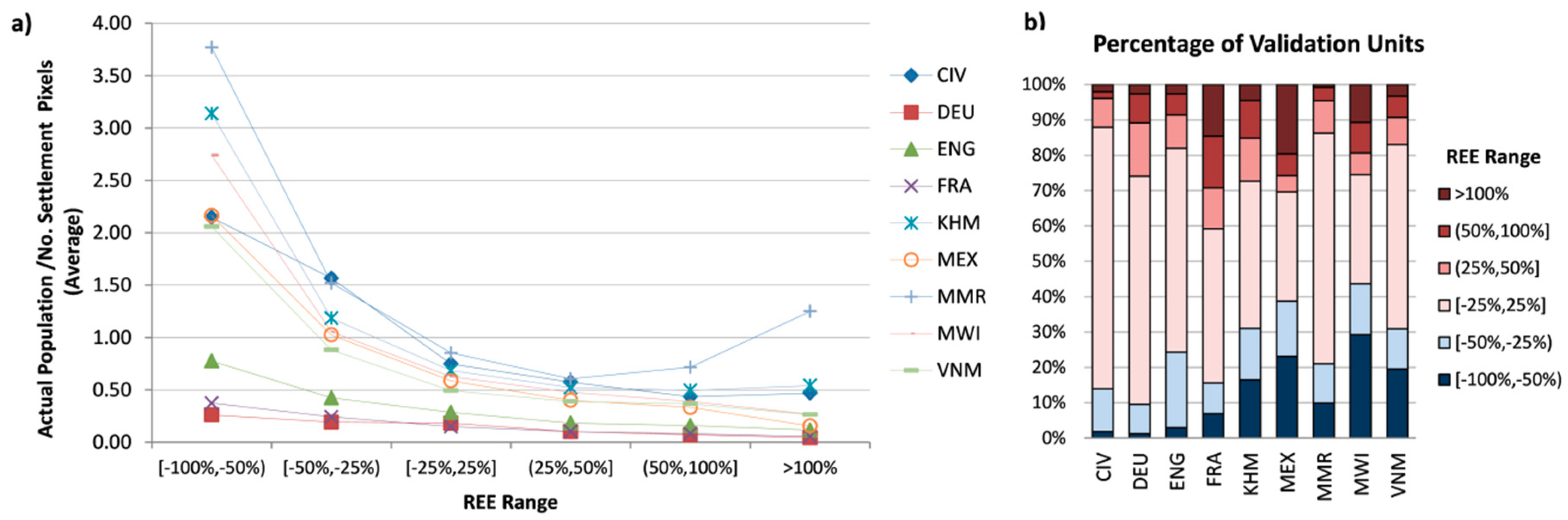
| REE Ranges | Description |
|---|---|
| [−100%, −50%) | Greatly underestimated |
| [−50%, −25%) | Underestimated |
| [−25%, 25%] | Accurately estimated |
| (25%, 50%] | Overestimated |
| (50%, ≥100%] | Greatly overestimated |
| SSC Index Class | Description |
|---|---|
| Low (>0–1) | Small size settlements and low coverage of the total area of the input units |
| Medium [1–1.8) | Mix of small and medium size settlements and medium coverage of the total area of the input units |
| High [1.8–10) | Mix of medium and large size settlements with high coverage of the total area of the input units |
| WSF-2015-Density | WSF-2015 | |||||||||||
|---|---|---|---|---|---|---|---|---|---|---|---|---|
| Country ISO | Average Population | Analysis | No. of Input Unit | No. of Validation Units | MAE | MAPE (%) | RMSE | R2 | MAE | MAPE (%) | RMSE | R2 |
| CIV | 43,910.16 | I | 110 | 517 | 10,029.04 | 22.84% | 40,198.00 | 0.7803 | 10,375.16 | 23.63% | 44,814.26 | 0.7224 |
| II | 35 | 11,851.45 | 26.99% | 41,343.98 | 0.7725 | 11,862.96 | 27.02% | 45,593.19 | 0.7130 | |||
| III | 1 | 15,016.82 | 34.20% | 47,045.80 | 0.5684 | 15,118.44 | 34.43% | 50,124.64 | 0.3891 | |||
| DEU | 7145.64 | I | 402 | 11,291 | 828.86 | 11.60% | 2261.67 | 0.9975 | 984.10 | 13.77% | 2824.88 | 0.9961 |
| II | 16 | 1897.35 | 26.55% | 12,580.46 | 0.9316 | 2281.22 | 31.92% | 14,409.45 | 0.9094 | |||
| III | 1 | 2481.30 | 34.72% | 23,280.14 | 0.9170 | 2999.64 | 41.98% | 26,407.33 | 0.9010 | |||
| EN | 8007.11 | I | 326 | 6791 | 2218.00 | 27.70% | 3309.71 | 0.1744 | 2347.93 | 29.32% | 3401.02 | 0.1415 |
| II | 9 | 2776.75 | 34.68% | 4310.88 | 0.1000 | 3208.51 | 40.07% | 4619.30 | 0.0474 | |||
| III | 1 | 3098.81 | 38.70% | 4666.95 | 0.0634 | 3642.90 | 45.50% | 5017.18 | 0.0167 | |||
| FRA | 1761.26 | I | 96 | 36,562 | 589.00 | 33.44% | 4605.53 | 0.8777 | 685.47 | 38.92% | 5242.17 | 0.8352 |
| II | 22 | 702.31 | 39.88% | 9543.18 | 0.7698 | 817.24 | 46.40% | 10,950.33 | 0.6333 | |||
| III | 1 | 821.41 | 46.64% | 11435.96 | 0.5279 | 954.06 | 54.17% | 12495.90 | 0.3390 | |||
| KHM | 9426.99 | I | 197 | 1633 | 3425.38 | 36.34% | 4898.26 | 0.6174 | 3241.26 | 34.38% | 4694.16 | 0.6204 |
| II | 25 | 4325.54 | 45.88% | 6680.15 | 0.5244 | 4078.17 | 43.26% | 6027.73 | 0.5371 | |||
| III | 1 | 4738.49 | 50.27% | 8363.82 | 0.5333 | 4343.88 | 46.08% | 6270.24 | 0.5662 | |||
| MEX | 2915.00 | I | 2456 | 65,477 | 954.40 | 32.74% | 2424.57 | 0.3841 | 1031.51 | 35.39% | 2599.99 | 0.3672 |
| II | 32 | 1080.44 | 37.06% | 2440.33 | 0.3176 | 1194.89 | 40.99% | 2611.97 | 0.3162 | |||
| III | 1 | 1719,04 | 58.97% | 30507.37 | 0.2326 | 1702,60 | 58.41% | 3464.93 | 0.2604 | |||
| MMR | 76,263.92 | I | 75 | 330 | 32,257.60 | 42.30% | 47,374.91 | 0.8214 | 34,301.82 | 44.98% | 49,602.98 | 0.7986 |
| II | 15 | 41,755.91 | 54.75% | 58,807.41 | 0.7611 | 44,506.83 | 58.36% | 64,708.38 | 0.7071 | |||
| III | 1 | 83,960.45 | 110.09% | 111,546.15 | 0.5243 | 66,606.76 | 87.34% | 88,449.93 | 0.4051 | |||
| MWI | 1371.73 | I | 357 | 12,550 | 712.08 | 51.91% | 1038.03 | 0.3231 | 687.40 | 50.11% | 1001.41 | 0.3290 |
| II | 32 | 795.36 | 57.98% | 1219.17 | 0.1732 | 766.46 | 55.88% | 1177.45 | 0.2050 | |||
| III | 1 | 836.53 | 60.98% | 1310.94 | 0.1924 | 792.69 | 57.79% | 1182.53 | 0.2423 | |||
| VNM | 135,824.99 | I | 63 | 688 | 46,646.67 | 34.34% | 76,804.15 | 0.6018 | 47,837.20 | 35.22% | 87,481.13 | 0.5218 |
| II | 6 | 57,187.23 | 42.10% | 94,536.29 | 0.4317 | 61,288.84 | 45.12% | 99,151.92 | 0.3578 | |||
| III | 1 | 61,323.29 | 45.15% | 95,472.76 | 0.3617 | 63,825.03 | 46.99% | 100,829.93 | 0.2636 | |||
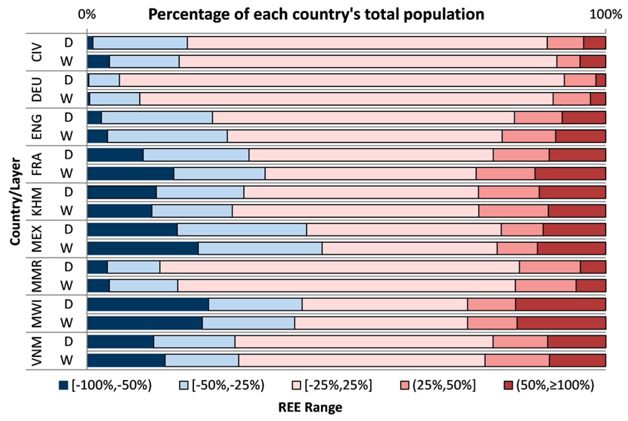
| REE Range | [−100%, −50%) | [−50%, −25%) | [−25%, 25%] | (25%, 50%] | (50%, ≥100%] | ||||||
|---|---|---|---|---|---|---|---|---|---|---|---|
| D | W | D | W | D | W | D | W | D | W | ||
| CIV | %Population | 1.11% | 4.30% | 18.22% | 13.44% | 69.40% | 72.84% | 6.98% | 4.47% | 4.29% | 4.95% |
| DEU | %Population | 0.34% | 0.51% | 5.90% | 9.63% | 85.78% | 79.69% | 6.05% | 7.19% | 1.92% | 2.97% |
| ENG | %Population | 2.78% | 3.94% | 21.40% | 23.09% | 58.22% | 53.00% | 9.21% | 10.30% | 8.39% | 9.67% |
| FRA | %Population | 10.82% | 16.73% | 20.42% | 17.57% | 47.06% | 40.70% | 10.79% | 11.34% | 10.92% | 13.66% |
| KHM | %Population | 13.35% | 12.50% | 16.87% | 15.48% | 45.23% | 47.55% | 11.73% | 13.40% | 12.82% | 11.07% |
| MEX | %Population | 17.37% | 21.42% | 24.97% | 23.90% | 37.50% | 33.73% | 8.09% | 7.76% | 12.07% | 13.19% |
| MMR | %Population | 3.92% | 4.27% | 10.14% | 13.22% | 69.30% | 65.06% | 11.74% | 11.73% | 4.92% | 5.73% |
| MWI | %Population | 23.44% | 22.23% | 18.03% | 17.80% | 31.87% | 33.33% | 9.25% | 9.54% | 17.41% | 17.11% |
| VNM | %Population | 12.84% | 15.04% | 15.66% | 14.20% | 49.78% | 47.47% | 10.50% | 12.43% | 11.23% | 10.86% |
| Low SSC Class | Medium SSC Class | High SSC Class | |||||||
|---|---|---|---|---|---|---|---|---|---|
| RMSE (D) | RMSE (W) | %Diff. | RMSE (D) | RMSE (W) | %Diff. | RMSE (D) | RMSE (W) | %Diff. | |
| CIV | 6195.88 | 5824.85 | −6.17% | 13,385.74 | 9893.41 | −30.00% | 121,500.76 | 138,430.55 | +13.03% |
| DEU | 598.65 | 701.99 | +15.89% | 1169.94 | 1422.94 | +19.51% | 1715.78 | 2100.37 | +20.16% |
| ENG | 2449.15 | 2879.85 | +16.16% | 2580.89 | 3013.39 | +15.46% | 2908.04 | 2980.60 | +2.46% |
| FRA | 517.12 | 647.56 | +22.40% | 975.40 | 1207.01 | +21.03% | 4391.66 | 5124.74 | +15.41% |
| KHM | 4041.02 | 3785.02 | −6.54%) | 3536.39 | 3084.83 | −13.64% | 6372.06 | 6443.97 | +1.12% |
| MEX | 892.80 | 874.05 | −2.12% | 2107.69 | 2253.53 | −6.69% | 2376.74 | 2626.13 | +9.97% |
| MMR | 33,452.74 | 34,943.76 | +4.36% | 39,432.66 | 32,580.79 | −19.03% | 43,682.69 | 59,832.04 | +31.20% |
| MWI | 819.79 | 768.93 | −6.40% | 778.43 | 831.73 | +6.62% | 1150.90 | 12,20.03 | +5.83% |
| VNM | 47,476.56 | 43,030.73 | −9.82% | 32,471.05 | 27,000.96 | +18.40% | 63,679.29 | 65,272.30 | +2.47% |
© 2019 by the authors. Licensee MDPI, Basel, Switzerland. This article is an open access article distributed under the terms and conditions of the Creative Commons Attribution (CC BY) license (http://creativecommons.org/licenses/by/4.0/).
Share and Cite
Palacios-Lopez, D.; Bachofer, F.; Esch, T.; Heldens, W.; Hirner, A.; Marconcini, M.; Sorichetta, A.; Zeidler, J.; Kuenzer, C.; Dech, S.; et al. New Perspectives for Mapping Global Population Distribution Using World Settlement Footprint Products. Sustainability 2019, 11, 6056. https://doi.org/10.3390/su11216056
Palacios-Lopez D, Bachofer F, Esch T, Heldens W, Hirner A, Marconcini M, Sorichetta A, Zeidler J, Kuenzer C, Dech S, et al. New Perspectives for Mapping Global Population Distribution Using World Settlement Footprint Products. Sustainability. 2019; 11(21):6056. https://doi.org/10.3390/su11216056
Chicago/Turabian StylePalacios-Lopez, Daniela, Felix Bachofer, Thomas Esch, Wieke Heldens, Andreas Hirner, Mattia Marconcini, Alessandro Sorichetta, Julian Zeidler, Claudia Kuenzer, Stefan Dech, and et al. 2019. "New Perspectives for Mapping Global Population Distribution Using World Settlement Footprint Products" Sustainability 11, no. 21: 6056. https://doi.org/10.3390/su11216056
APA StylePalacios-Lopez, D., Bachofer, F., Esch, T., Heldens, W., Hirner, A., Marconcini, M., Sorichetta, A., Zeidler, J., Kuenzer, C., Dech, S., Tatem, A. J., & Reinartz, P. (2019). New Perspectives for Mapping Global Population Distribution Using World Settlement Footprint Products. Sustainability, 11(21), 6056. https://doi.org/10.3390/su11216056