Abstract
The direction and environment of photovoltaics (PVs) may influence their energy output. The practical PV performance under various conditions should be estimated, particularly during initial design stages when PV model types are unknown. Previous studies have focused on a limited number of PV projects, which required the details of many PV models; furthermore, the models can be case sensitive. According to the 18 projects conducted in 7 locations (latitude 29.5–51.25N) around the world, we developed polynomials for the crystalline silicon PV energy output for different accessible input variables. A regression tree effectively evaluated the correlations of the outcomes with the input variables; those of high importance were identified. The coefficient of determination, indicating the percentage of datasets being predictable by the input, was higher than 0.65 for 14 of the 18 projects when the polynomial was developed using the accessible variables such as global horizontal solar radiation. However, individual equations should be derived for horizontal cases, indicating that a universal polynomial for crystalline silicon PVs with a tilt angle in the range 0°–66° can be difficult to develop. The proposed model will contribute to evaluating the performance of PVs with low and medium tilt angles for places of similar climates.
1. Introduction
There is an increasing concern regarding energy resources, energy use, and its probable effects on the environment. Urban areas require a large amount of energy to operate, and buildings consume a significant portion of this energy. Hong Kong, for example, utilizes imported nuclear power and fossil fuels [1], and most of the energy is used by the residential and commercial buildings [2]. The combustion of fossil fuels is the leading cause of air pollution, respiratory illnesses, and greenhouse gases [3]. Renewable energy resources can be a clean and safe alternative to conventional energy resources with the increasing energy demands and an eco-protection consensus. Solar energy is abundant in many high-altitude and subtropical regions [4], and can be used as a clean, renewable resource in the city environment via building integrated photovoltaic (PV) panels [5] at various tilt angles and azimuthal directions. PV panels installed on vertical or inclined building facades and overhangs can be installed on larger areas to reduce building heat gains [6]. For low and zero energy buildings, the energy produced by PV panels is essential to cover their basic energy needs.
Accurate estimation of PV energy output in hourly or even sub-hourly intervals is essential for evaluating the energy output potential and fluctuation impacts on the electricity grid [7]. The nameplate energy output of a PV panel is tested using the standard test conditions (STC) of 1000 W/m2 irradiance, 25 °C cell temperature, and 1.5 air mass. The real operational environment for PV panels, however, may be different from the STC, making the real-time energy output different from the nameplate value [8]. On-site measurement, in theory, is most reliable for evaluating PV panel performance [9]. However, field measurements are not available before the PV is installed, and it is not practical to conduct long-term field tests for every engineering project. The solar angle, temperature, and irradiance may vary with the weather, season, and time of day, resulting in dynamic impacts on the PV cells that can be different from the STC in practice. In addition, building-integrated PV panels can tilt and face various directions. Thus, the difficulty in evaluating the performances of PV panels may vary with each case. Without field measurements, the energy output of PV panels facing different directions, in the long run, will need to be estimated by the climatic indices that are accessible from the weather file.
Theoretically, PV operating efficiency can be estimated by the environmental and inherent parameters of the PV panel; however, the latter should be determined by a specific PV model [10,11,12]. The parameters of a PV panel may not be available, especially in the early stages of the project when energy-saving strategies can be adopted with minimal design and construction cost. Developing a non-case-sensitive model for estimating silicon PV panel energy outputs according to the climatic variables may contribute to evaluating the PV energy output potential during the early stages of the project. Previously, many empirical and semi-empirical models were developed [13,14,15] to estimate PV energy output in outdoor environments. Most models were developed using the PV energy output data from a limited number of projects [16], making the models somehow case-sensitive. Developing models using data from various PV panels with different tilt angles and climate conditions can result in more universal conclusions. This may involve several large databases and input variables. This Big Data problem is usually solved by machine learning approaches [17,18] that may develop accurate non-linear models from large datasets for engineering problems [19]. Artificial neural network (ANN) [20] have frequently been used for estimating PV energy output in many studies. However, the ANN develops black box models that may contain hundreds of weight and bias factors, making it difficult to interpret and transplant, but easy to become overfitted. Several existing ANN studies were developed using data obtained from a few PV projects [20,21], resulting in neural network models that may be case-sensitive. Thus, using ANN in a new project can be theoretically and technically challenging. Persson et al. [22] proposed an approach for forecasting the PV powers using the boosted regression tree with 42 solar cells in Nagoya Bay, Japan. However, the models that forecast the future PV performance was partly based on the previous performance data, which is not appropriate for the early-stage evaluations using ‘typical’ weather data. Moreover, the boosted model was developed using up to 200 regression trees, resulting in a larger number of coefficients than that for ANN, causing difficulties for it to be used elsewhere. In this connection, it is expected that a simple and robust model will be developed that estimates the performance of the silicon crystalline PV cells in different routine tilt angles and azimuthal directions that can be applied for engineering use in early design stages.
The multi-variable curve fitting can be an effective approach for the problem, considering the limitations of machine learning. The outcomes are in the form of simple equations, and thus are unlikely to be overfitted, and should be robust, especially for new PV projects. The equations are easier to use and faster to compute compared with many machine learning approaches [22,23]. However, selecting an appropriate format of the empirical models for curve fitting relies on the developer’s experience. The classical polynomials of second or higher orders can demand a large number of coefficients and terms when an excessive number of input variables are involved. It is essential to identify the input variables that are of the highest importance for concise polynomial expressions. A previous work studied the correlation between the PV temperature (and ultimately energy output) with the climatic variables using the feature selection and mutual information methods [24]. However, data of only one place was used, and the results gave the correlation factors only. The regression tree (RTree) approach [25] can be used to identifying the input variables of high importance. The RTree is a classical and effective approach used to correlate the target output with the other readily accessible inputs. The contributions of each input in explaining the output can be interpreted by the structure of the RTree model [26]. This work correlated the real-time PV energy output with the simultaneously recorded meteorological data of as much as 17 silicon crystalline PV projects over 7 worldwide regions. Specially, importance of the input variables to the PV performance estimation were evaluated to remove those variables of a low significance using the RTree approach. This saved the cost of measurement, model development, and curve fitting. The performances of the polynomials in the first and second orders using the identified input variables were evaluated, and their advantages and limitations are discussed.
2. Data Collection of PV and Solar Radiation
This study used the meteorological data and the PV energy output field measurements. The PV performance data included 15 American projects and 2 German projects from the PVOutput website [27]. All projects used silicon crystalline PV cells that shared similar responses to the climatic conditions [14]. The meteorological data obtained from five different locations in the USA were recorded by the Measurement and Instrumentation Data Centre (MIDC) of the National Renewable Energy Lab (NREL), USA. Weather data of the two German (DE) locations were acquired from the server of the Deutscher Wetterdienst Climate data centre (CDC) [28]. Data from the Centre for Sustainable Energy Technologies (CSET) of the University of Nottingham, Ningbo, China (UNNC), consisted of an independent database for model testing that included the PV energy output, solar radiation, and air temperature. Table 1 lists the weather station details of the pyranometer and pyrheliometer accuracies. The stations covered a wide range of climate zones from humid to arid. Most of the stations measured the solar irradiance using the high accuracy thermopile meters in the secondary standard or the first class. Scanning pyrheliometer and pyranometer (SCAPP) represents a low-cost silicon meter that measures the diffuse and direct solar irradiance with moderate accuracy [29]. The dry-bulb air temperature and wind speed, as contributors to the PV cell temperature variation, were acquired as well. Two of the MIDC measurement stations (CO and AZ) in west USA were characterised by desert or continental climate. The weather station in Oregon (OR) was of a marine climate, and the station in Tennessee (TN) was of a subtropical climate. The weather data measurements by the two German stations (NW and HH) were in the temperate maritime climate zone. The USA weather data were recorded every minute, whereas the weather data from Germany and UNNC were recorded in 10 min intervals. Table 2 lists the system size, panel brand, tilt angle, azimuth angle, and weather data of the PV projects in different places. The majority of the PV energy measurements were performed in 5 min intervals, whereas the Germany project data were averaged over 10 min for consistency with the weather data. The PV energy output of UNNC was in the 2 min interval and averaged over 10 min. The tilt angles of the PV projects ranged from 0 (horizontal) to more than 60°, covering most of the PV installation routines. The tilt angles of many PV panels under study were different from the site latitude, and their azimuth directions were not in line with the equator direction. This was due to the site restrictions, especially when the panels were installed on buildings. The tilt angles of 14 projects were less than 40°, and the azimuth angles of most of the PV panels ranged from 140° to 225° for harvesting solar energy in the northern hemisphere. The PV panels considered in this study thus represented projects in various worldwide climate zones and various tilt angles. The energy outputs of each project were normalized by its capacity in STC.

Table 1.
Specifications of the stations measuring the weather data. CO: Colorado; OR: Oregon; AZ: Arizona; TN: Tennessee; NW: Nordrhein-Westfalen; HH: Hamburg; DE: Germany sites; MIDC: Measurement and Instrumentation Data Centre; CDC: Deutscher Wetterdienst Climate data centre; CN: China; UNCC: University of Nottingham, Ningbo, China; SCAPP: scanning pyrheliometer and pyranometer [29].
Table 2.
Specifications of the projects for the Silicon crystalline photovoltaic (PV) panel performance data.
There may be inaccurate recordings in the raw data measurements that may have resulted from the pyranometer cosine response, improper shadow band or shadow ball positioning, or even a bird nesting. Thus, the data quality was evaluated by referring to a guide of the International Commission of Illumination (CIE) [34]. The global, direct, and diffuse solar irradiance were essential variables for calculating the solar energy on the PV panels, which contributed to the power production. The missing irradiance component among direct, diffuse, or global, if any, was calculated using the other two components. The testing criteria comprised five levels that are listed as follows: Level 0 provided the amount of data recorded during the daytime when the solar altitude was higher than 0. For German sites that had only the diffuse and direct measurements (yet recorded as diffuse and global) by SCAPP, quality control Level 3 was skipped. Levels 4 and 5 removed the power output rates and PV panel efficiencies that were unrealistically high. A relatively flexible criterion was set for Level 5 because the efficiency was relevant to the PV panel size and solar energy on the PV panels that may have resulted from the erroneous panel information. Table 3 specifies the data quantity and the results of quality control for each site. From the PVOutput website, the PV panel performance data from the end of 2017 to June 2018 were acquired. The data available covered half a year from winter to summer. There were roughly 11,800–18,900 PV performance data samples for most of the United States PV projects, and 2600–3150 data samples in the 10 min interval from the PV projects in Germany. The significant data quantity reduction from Levels 3 to 5 for Projects 4 and 11 were because their PV outputs were measured with an interval of 15 min. In total, 250,788 datasets of PV projects in different climate zones were used for the analysis.
Table 3.
Data quality controls for the 18 silicon crystalline PV projects.
Level 0: Solar altitude angle αS should be greater than 0°.
Level 1: αS should be greater than 4°;
Horizontal global solar irradiance (EHG) should be greater than 20 W/m2.
Level 2: EHG should be greater than 0 and less than the extraterritorial horizontal solar irradiance (EHE);
The horizontal diffuse sky irradiance (EHD) should be greater than 0 and less than 0.5 EHE;
The direct beam irradiance (ENB) should be greater than or equal to 0 and less than the extraterritorial beam irradiance (ENE).
Level 3: For sites with direct, diffuse, and global measurements, EHG should be within (EHD + ENB sinαS) ± 15%;
For sites with global and diffuse measurements only, EHD should not be greater than EHG.
Level 4: The ratio of PV energy output to its capacity (r) defined as the ratio of energy output to energy output at STC should be greater than 0.01 and less than 1.
Level 5: The efficiency of the PV panel defined as the ratio of the energy output to estimated solar irradiance on a panel should be less than 0.3.
3. Methodologies
Figure 1 summarizes the overview of the current research. Firstly, the structure complexity of the RTree, determined by Lmin, was optimized to avoid overfitting. The importance of each potential input variable was studied by the RTree in the optimized complexity levels. The contributions of the input variables to the output estimation were quantified, and the model performance by different input combinations was tested. The selected variables of high importance were used to develop polynomials to estimate the PV energy output by multi-variable regressions.
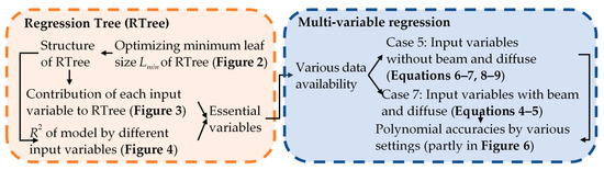
Figure 1.
The research methodology map and correlations between the equations and figures. RTree: regression tree.
The RTree algorithm used a sequence of binary partitions (splits) to separate the datasets into various groups according to the input variables (x1, x2, …, xn). Figure 2 illustrates a split that divided the NA datasets of Node A into two child groups of Nodes B and C by the threshold of a variable (xj). xj and its threshold were determined to minimise the variance of the output. Equation (1) defines the reduction of variance owing to the split, where Var indicates the variance of the datasets in each node. ͞rA, ͞rB, and ͞rC are the average energy output rates for the datasets of Nodes A, B, and C, respectively. In the case of missing data, a substitute variable for xj can be determined as the surrogate. The variance of a node denotes how far the datasets are from their averages, which can be reduced by repeating the binary split several times. The approach classifies the datasets with a similar output of r into the same terminal node and represents them using their average value. The splitting stops when certain criteria, such as the datasets in the terminal node (leaf) being less than a minimum size (Lmin), are met. A lower Lmin would lead to a more complicated RTree, which performs in-depth classifications for less output variance in the terminal node. However, an overly complicated model may be over-fitted and misled by the measurement errors and features that are not universal. Therefore, the RTree performance was tested by setting Lmin as 20, 40, …, 100, 200, …, 500, 1000, …, 2500, 5000, …, 10,000 for the model performances at different complexity levels.
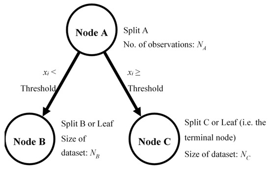
Figure 2.
Single split of the regression tree (RTree).
Selecting the appropriate input variables for estimation is another critical issue. Using fewer input variables can reduce the model complexity and save the data measurement cost for other users. It is essential to develop the RTree model using input variables carrying equivalent “knowledge” of the PV at different tilt angles and directions to ensure that the RTree model can adapt to a maximum range of projects. Fortunately, the variable importance can be estimated by the developed RTree models according to the variance reduction given in Equation (1). A variable xi (or its surrogate) may determine various splits of the developed RTree, and the total variance reductions by such splits indicate the contribution of xi (or its surrogate) to the RTree. This implies that all the surrogating variables can gain importance when they contribute to a split. A variable can be more critical to the RTree if it is the criteria of many splits and contributes to significant output variance reductions. Alternatively, testing the model performance using a part of the input variable can be a more straightforward way to evaluate the variable importance. Table 4 presents the input variable combinations for the test, where Ecell represents the global solar irradiance on the PV panel, and Kcell is the diffuse fraction of the global irradiance on the PV panel (Ecell). Ecell and Kcell were determined by the well-acknowledged Perez 1990 model [35]. ZS is the solar zenith angle and σ is the solar incidence angle on the PV panel. Variables of Case 1 in Table 4 are irrelevant to the PV panel direction, which represented the initial project stage when the PV installation details could not be fully specified. Cases 2 and 3 compared the performance of models that were developed using the solar irradiance and clearness index on the PV panel against those using the variables on the horizontal ground. Because the weather data may not be fully available for many places, Cases 4 to 8 tested the model performance when several variables of the weather data were removed during the RTree development. Cases 4 to 6 tested the accuracy of the model that was developed without either the air temperature Tair or the wind velocity, or both as the input variable. Case 7 evaluated the model performance when only the global horizontal irradiance was available as the fundamental solar radiation measurement. The solar irradiance on the tilted surface could not be determined accurately in such a case. Case 8 evaluated the model when the solar radiation data was not entirely available. For all tests, the solar altitude angle was assumed to be always accessible and was determined by the local time, latitude, and longitude.
Table 4.
Input variable combinations for the RTree development and accuracy evaluation.
One issue faced by the RTree was the model validity for new data, which may be lower than expected if the training data was insufficient. A database for training should be comprehensive enough so that the developed model can perform well for the new data. The PV panels may have various installation angles in different climate zones and operate in different seasons. It is essential to study the RTree performance for new PV panels at angular directions that are different from those in the projects under study. This work used cross-validation to evaluate the model accuracy. For each of the 17 PV projects, the energy output rate (r) was estimated by the RTree model that was developed using the other 16 projects. Model performance evaluations for different Lmin and input variable combinations were enhanced by bootstrapping tests [36] for less uncertainty due to the random input and output database selection. The performance of the model was evaluated by the ratio of the root mean square error to the measurement average (%RMSE) given in Equation (2) to the coefficient of determination (R2) given in Equation (3). R2 shows the percentage of the output variance that can be estimated from the input data using the derived models. R2 can take zero as minimum and one as maximum, and it identified the model accuracy in a straightforward manner.
The RTree with the optimised r variance in the terminal nodes can still be highly complex, consisting of many splits and coefficients. Pruning the developed RTrees may remove the excessive branches that contain overwhelming coefficient quantities but make few contributions to the model accuracy. A classical approach to remove an RTree branch is to balance out the RTree model complexity reduction against the potential error. Reduction of the RTree complexity was denoted as the number of terminal nodes in the branch to be removed. The ratio of the extra error to number of terminal nodes for an RTree branch to be removed was defined as the complexity parameter α for the node. The prune starting with the low α would remove RTree branches that were more complex, thereby resulting in minimal error in the output.
4. Results and Discussion
Figure 3 illustrates the R2 and %RMSE of the PV energy output rate (r) for different Lmin settings. The bottom and top box edges in the figure represent the 25th percentile (q1) and 75th percentile (q3) [37] of the 100 model developments by bootstrapping for each Lmin setting. The bottom and top whisker edges represent the far outside boundaries of the bootstrapping results, which are defined as q1 − 3(q3 − q1) and q3 + 3(q3 − q1) [38], respectively. Such a boundary definition will cover more than 99.5% of the results of the bootstrapping tests if the R2 and %RMSE values are in a normal distribution. Thus, results outside the Whisker edges can be considered as outliers and were not plotted. The figure indicates an improvement of the model accuracy when Lmin increased from 20 to approximately 1000, and then the accuracy decreased gradually when Lmin increased further. The models developed by Lmin = 500 and 1000 were similar in accuracies, yet the later was simpler. The 1000 datasets accounted for 0.373% of the entire database. R2 was approximately 0.745 for the RTree developed by Lmin of 1000, indicating that approximately 74.5% of the data could be explained. The variation trend of %RMSE for different hidden neurons was opposite to that of R2. The minimum %RMSE of the RTree developed by setting Lmin as 1000 was approximately 37.7% considering an average r of 0.3546 for the datasets of all 17 stations. The figure implies that Lmin = 1000 is appropriate for testing the subsequent RTree developments and performance evaluations.
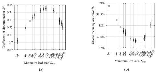
Figure 3.
(a) R2 and (b) %RMSE of the 50 bootstrapping tests of the RTree in different Lmin settings.
Figure 4 illustrates the contributions of the input variables in estimating the PV energy output rate according to the RTree with and without surrogates. All input variables were assumed to be available and the process was repeated by conducting 5000 bootstrapping tests. The contributions, as observed in the two figures, were different but exhibited a few consistencies. Figure 4a,b indicates that Ecell provided the highest contributions to the RTree model, which were 94.5% (Figure 4a) and 22% (Figure 4b). This disparity implies that Ecell can be partly replaced by other variables, such as EHG and ENG, whose importance was less than 0.4% in Figure 4a in comparison with that of Ecell in Figure 4b. It was not surprising that the contributions of Ecell and Kcell were higher than those of EHG, EHD, and ENB because the former two were more closely related to the PV panel. The solar incidence angle cosσ was of a lower importance compared to other variables in Figure 4a. The variable for the RTree with a surrogate in Figure 4b was of moderate importance, probably because Ecell was not directly available. The contributions of EHD and v were low for the RTree models developed either with or without surrogates. Tair was of good accessibility by routine measurements; however, its contribution in estimating r was either moderate or low for the RTree. This is because the PV cell temperature was vastly affected by both Tair and solar radiation.
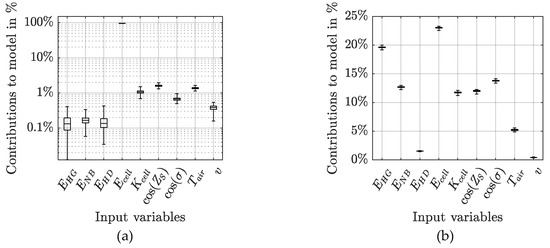
Figure 4.
Contributions of the variables to the RTree model (a) without and (b) with surrogates.
Figure 5 shows the R2 of RTree through 100 bootstrapping tests using a few of the input variables. Lmin was set as 1000 on the basis of the data presented in Figure 3. R2s of Cases 3 to 6 were greater than 0.76 and Cases 3 and 5 exhibited the best performances. R2 was approximately 0.51 for Case 8 when solar radiation was completely unavailable, which was considerably lesser than the lower limit shown in the figure. The difference of R2 between Cases 1 and 3 exceeded 0.06 (Figure 5); this indicated that it was difficult to estimate the PV performance without specifying its directions in the initial design stage. R2 of Case 3 was higher than that of Case 2; the difference was approximately 0.015. The best performances were exhibited by Cases 3 and 5 because the RTrees were developed on the basis of the irradiance variable with reference to the PV panel. The R2 of Case 2 was close to those of Cases 3 and 5, probably because the PV panels of most projects were similar to each other; furthermore, the on-panel irradiance could be estimated by the horizontal solar irradiance via the RTree model structure. R2s of Cases 4, 5, and 6 in Figure 5 show that the air temperature might have slightly affected the model, whereas the wind speed can be neglected to save the data measurement costs without influencing the accuracy of the model. Case 7 shows that approximately 74% of data can be estimated by global horizontal solar irradiance measurements using the RTree model. Finally, as Case 5 indicated, the five variables of Ecell, Kcell, ZS, σ, and Tair were used to develop the models required for estimating the real-time PV energy output rate. In addition, models developed using EHG, ZS, σ, and Tair of Case 7 without direct or diffuse components were also tested for data accessibility.
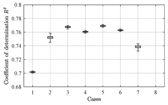
Figure 5.
RTree accuracies for the eight cases in Table 4 when a few of the variables were available; R2 of Case 8 was approximately 0.51, far less than the lower limit of 0.68.
The polynomials were developed using the identified variables of high importance to evaluate the PV performance. Variables of low importance were neglected to simplify the equation. Equations (4) and (5) were developed using the five variables (Ecell, Kcell, cos(ZS), cosσ, and Tair) of Case 5 from projects 1 to 17, and Equations (6) and (7) were developed by the four variables (EHG, cos(ZS), cosσ, and Tair) of Case 7. The latter was essential when the direct and diffuse solar irradiance components were not available. The input variables were standardized using Z-score normalization as summarized in Table 5, and X1 to X5 represent the standardized variables. The coefficients of the second order polynomials are listed in Table 6. The second order coefficients (Ci,j) were close to zero for the five-variable polynomial, and X32, X42 and X52 were zero. The low Di,j values implied that the correlation was evidently linear.
Table 5.
Variables for model development that are standard by the Z-score normalization.
Table 6.
Coefficients Ci,j of the second order polynomial.
Figure 6 demonstrates the average r when each input variable was within a series of local ranges represented by their medians on the basis of PV projects 1 to 17. The output r could take different values when an input variable was maintained constant while other variables were not. In this connection, the r values for each subplot were averaged 100 times; each time, 1% of the local data was used. The values of r obtained from the four-variable model (Case 7) were plotted; the five-variable model (Case 5) exhibited better performance. The figures show the dependency of PV energy output on the input variables and estimation accuracies. Figure 6d also presents the variation trend of Ecell with Tair. Figure 6 depicts that r, estimated using the second order polynomial, are in good agreement with the practical measurements. The efficiencies at EHG greater than 1000 W/m2 were overestimated; however, EHG rarely exceeded 1000 W/m2. Cases with EHG of approximately 1000 accounted for only 3.8% of the total datasets, and the extremely high values of EHG were measured during short summer periods. The smoothed r increased significantly over the ranges of EHG and cosZS, as shown in Figure 6a,b, and moderately over the cosσ range as shown in Figure 6c. Such trends were consistent with their level of importance shown in Figure 4 and Figure 5. Figure 6a reveals that the smoothed r increased from 0 to 0.8 as EHG increased from 0 to over 1000 W/m2, probably because the PV cells were insensitive to the low sunlight. However, r reduced to 0.6 as EHG increased further, possibly because of the high panel temperature. Figure 6b,c illustrates that the smoothed average r reduced from 0.8 and 0.6, respectively, to less than 0.1 when solar zenith and incidence angles increased from less than 10° to 90°. According to Figure 6b, the energy output rate peaked at cos(ZS) = 0.975, which corresponded to ZS = 13°, probably because most data were obtained from the PV cells with tilt angles lesser than 30°; many PV cells were horizontally installed. In addition, the solar irradiance was stronger at high cosZS (i.e., low air mass) compared with that at low cosZS. Figure 6d shows a gradual increase of r from 0.2 to 0.5 when Tair increased from 0 to 30, indicating a relatively low contribution of Tair to the model. The high air temperature over 30 °C corresponded to the substantial solar irradiance over 700 W/m2, which led to high energy outputs. However, the r of 700 W/m2 shown in Figure 6d was not as significant as that shown in Figure 6a because of the high cell temperature.
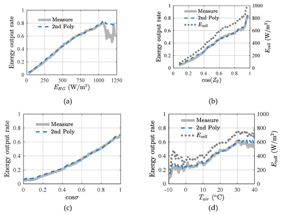
Figure 6.
Dependencies of the measured and PV energy output rate r by Case 7 settings for (a) horizontal global irradiance EHG; (b) cos (ZS); (c) cos σ; (d) air temperature Tair.
Figure 7 shows the accuracies (R2) of the first and second order polynomial equation models for different PV projects. According to Figure 7a, the accuracies of the linear (first-order) and second-order polynomials were comparable when the five variables of Case 5 (Ecell, Kcell, cosZS, cosσ, and Tair) were available. Compared with the first-order polynomial, the second-order polynomial slightly increased the accuracies of projects 2, 4, 5, 13, 17, and 18 of moderate and high tilt angles; however, it reduced the accuracies of the horizontal PVs of projects 6 and 8. Figure 7b shows the RTree and polynomial performances developed by EHG, cosZS, cosσ, and Tair. Ecell and Kcell that could be determined by the direct and diffuse components were not available, and EHG was used as an alternative. The second order polynomials evidently improved the accuracies for PV projects 4, 5, and 14–17. For the horizontal PV cells of projects 6, 8, and 9, however, the universal polynomials were invalid when the Ecell and Kcell were not available. This was probably because the polynomials focused on the PV projects where the tilt angles were approximately 20°–40°; this accounted for most of the datasets for the model development. The polynomials exhibited inconsistent performance for PV cells where the tilt angle exceeded 60°, as the R2 was higher than 0.7 for project 10, yet lower than 0.4 for project 4. Equations (8) and (9) were developed, in this connection, by data obtained from projects 6, 8, and 9 for horizontal PV panels only. The overall R2 of Equations (8) and (9) for projects 6, 8, and 9 were 0.70 and 0.72, respectively. The results can be compared to a classical model given in Appendix A.

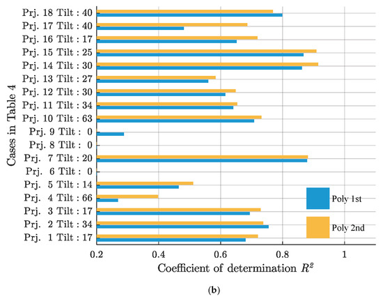
Figure 7.
R2 of the first- and second-order polynomials that were developed by (a) the five variables (Ecell, Kcell, cosZS, cosσ, Tair) of Case 5; (b) the four variables (EHG, cosZS, cosσ, and Tair) of Case 7. ‘Tilt’ means the tilt angle in degrees, ‘Prj.’ stands for project, which is described in Table 3.
Figure 8a–d presents the measured and estimated real-time r series of PV panels that were installed horizontally (project 8), and tilted by 20°, 30°, and 63° (projects 7, 14, and 10, respectively) on a typical day in 2018. The measured and estimated r of the independent testing dataset of UNNC were plotted as shown in Figure 8e. These projects were selected to represent those with a similar tilt angle. The four variables of Case 7 including EHG, cosZS, cosσ, and Tair were the input variables for the second order polynomial of Equations (7) and (9). Models developed by the five variables of Case 5 should be of higher accuracy on the basis of Figure 7. The period considered was between the end of spring and the beginning of summer. In all graphs, there were a few discontinuities at a few data points; this was because data were either missing or rejected by data quality control. There were only a few data points removed during the plotted period. The figures showed that the second order polynomial correctly estimated the r variation features for PV panels with different tilt angles and at various locations using solely the four readily accessible variables. The PV panels produced more solar energy around noon, owing to the abundant solar radiation and lower air mass. Figure 8a shows that r was overestimated by the polynomial that was developed using the entire dataset of projects 1 to 17. In such cases, Equation (9) should be used to accurately estimate the r of horizontal PV projects. This implicates that the polynomial can somehow be limited for complicated problems that involve PV cells of different features. The solar irradiances on Figure 8a,d fluctuated evidently and were slightly less accurate than that shown in Figure 8b,c,e. The r shown in Figure 8a,d was probably affected by various factors such as cloud coverage, indicating that the sky condition can help evaluate the real-time PV energy output. As shown in Figure 8d, the energy output was underestimated in the afternoon; slight overestimations were observed in the morning and at noon in Figure 8e.
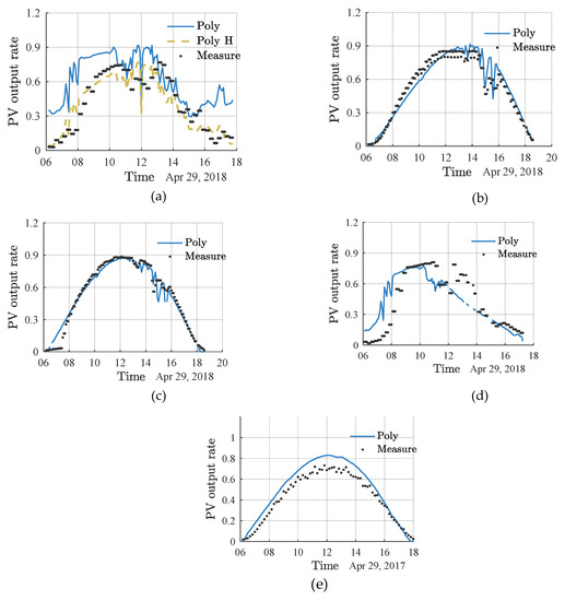
Figure 8.
Measured and estimated PV energy output rates during a typical day for (a) project 8 Fuzz4 House, horizontal PV panels; (b) project 7 Flecha Caida, panels tilted by 20°; (c) project 14 Rusch Ridge, panels tilted by 30°; (d) project 10 Kentucky, panels tilted by 63°; (e) independent dataset of UNNC, panels tilted by 30°. (y-axis is a ratio, and is dimensionless).
5. Conclusions
We developed polynomials to estimate the energy output of silicon crystalline PV panels in different locations and at various tilt angles. The input variables deemed crucial to the model estimation were identified using the RTree for model simplicity. The important variables included the solar irradiance and diffuse fraction on the PV panel (Ecell and Kcell), cosine solar zenith angle and incidence angle (cosZS and cosσ), and air temperature (Tair). The horizontal solar global irradiance could be used as an alternative for the Ecell and Kcell because their values are unavailable in many places around the world. The R2 values of the polynomials developed by the most relevant five variables were greater than 0.65 and 0.7 for projects 14 and 11, respectively, out of the 18 projects with different climates and in medium latitude regions. The model accuracy was slightly sacrificed when replacing Ecell and Kcell with the more accessible horizontal global solar irradiance EHG. There were 14 out of 18 PV projects with R2 over 0.65 when their r values were estimated using the second order polynomial. However, the polynomials were developed independently for solely horizontal PV projects. It is thus concluded that the polynomial model is generally not case-sensitive and should reliably estimate the energy output of new silicon PV panels with low and medium tilt degrees, facing various directions including southeast, south, and southwest. The proposed models could accurately estimate the long-term energy productions of silicon crystalline PV panels typically in places where the meteorological year database was accessible. The work provides essential knowledge regarding the designs of energy saving and renewable energy projects. In addition, it demonstrates an approach to estimate the outcomes of machine learning to develop polynomial equations. The findings were applicable for silicon crystalline PV cells only, which, however, represent most of the engineering projects and commercial uses nowadays.
Author Contributions
Conceptualization: D.H.W.L.; data curation: D.H.W.L., S.L., H.C., W.C., and I.Y.F.L.; funding acquisition: S.L. and D.H.W.L.; methodology: D.H.W.L., S.L., I.Y.F.L., and D.X.; resources: D.H.W.L.; software: S.L., H.C., and M.W.; supervision: D.H.W.L.; validation: S.L.; visualization: M.W.; writing—original draft: S.L.; writing—review and editing: S.L. and W.C.
Funding
The work was conducted under A Fundamental Study of Anisotropic Sky Radiance and its Effect on Building Envelopes in City Environments, supported by the National Natural Science Foundation of China (ID: 51808139).
Acknowledgments
The authors want to thank Dr. Isaac Yu Fat Lun from the University of Nottingham, Ningbo, China (UNNC), for helping us get access to the data available at the Centre for Sustainable Energy Technologies (CSET).
Conflicts of Interest
The authors declare no conflict of interest.
Nomenclature
Abbreviations
| ANN | Artificial neural networks |
| CIE | International Commission of Illumination |
| CDC | Climate data centre |
| CSET | Centre for Sustainable Energy Technologies |
| MIDC | Measurement and Instrumentation Data Centre of National Renewable Energy Lab |
| NREL | National Renewable Energy Lab |
| PV | Photovoltaic |
| RMSE | Root mean square error |
| RTree | Regression trees |
| SCAPP | Scanning pyrheliometer and pyranometer |
| STC | Standard test condition |
| UNNC | University of Nottingham, Ningbo, China |
Variables
| Ecell | Solar irradiance on PV cell |
| EHD | Diffuse solar irradiance on horizontal planes on the ground level |
| EHG | Global solar irradiance on horizontal planes on the ground level |
| ENB | The direct beam solar irradiance in the direction of the sun on the ground level |
| ENE | The extraterritorial direct beam solar irradiance in the direction of the sun (on the top of the atmosphere) |
| Kcell | Percentage of the diffuse irradiance on the PV cell |
| R2 | Coefficient of determination |
| r | Energy output rate of the PV cell, the ratio of real energy output to the nameplate value |
| Tair | Air temperature |
| ZS | Solar zenith angle |
| σ | Incidence angle of the sun to the PV plane |
ID of the weather station
| AZ | Arizona |
| CO | Colorado |
| DE | Germany sites |
| HH | Hamburg |
| NW | Nordrhein-Westfalen |
| NV | Nevada |
| OR | Oregon |
| TN | Tennessee |
| NV | Nevada |
Appendix A. Performance of a Classical Model
Equation (A1) gives a classical model that estimates the effect of the environment on the PV efficiency. This model needs the nominal operating cell temperature (TNOCT), which was tested by the manufacturer using 800 W/m2 solar irradiance on the cell (ENOCT), 20 °C surrounding air temperature, 1 m/s wind speed, and open back side installation. In Equation A1, ηref is the nameplate efficiency of the PV, η is the real-time efficiency determined by the environment, Ecell is the real-time irradiance on the PV panel, and Tref is the PV temperature at the standard test condition, which should be 25 °C. Coefficient β is set at 0.0045, as recommended by reference [14], according to a number of models. The estimation of Ecell needs the direct beam and sky diffuse radiation, which were less accessible than the horizontal global (EHG). The solar incidence angle on the plane (σ) is needed as well. ηref and TNOCT identifies the energy production and thermal features of the PV panel, and was determined by the product catalogs. Performance of Case 1 was not given because the panel model was not specified.
The R2 values in Table A1 show that the model was valid for most projects under study, yet became invalid for the others, and the R2 values of six projects were less than 0.5. An R2 lower than 0 meant the model estimation led to more uncertainties than the measurement average. The classical model outperformed the proposed equations (including those for tilt and horizontal cells) for projects 4 and 17 only, and was generally less accurate than the other cases. For project 18 that was not used in developing the new equations, R2 of the classical model was 0.57, which was lower than the R2 of the proposed case that almost reached 0.8. This indicates that the proposed model, in the form of one or two simple equations, was in good robustness for PV projects of different tilt angles.
Table A1.
The input coefficients and R2 values of the classical model for projects under study.
Table A1.
The input coefficients and R2 values of the classical model for projects under study.
| Project ID | Area (m2) | Project Name | Panel Brand and Model | TNOCT | ηref | R2 of Equation (A1) |
|---|---|---|---|---|---|---|
| 1 | N.G. | 5suns | Not given (N.G.) | - | - | - |
| 2 | 22.3 | Bayaud | LG 300N1K-G4 | 45 °C | 18.3% | 0.58 |
| 3 | 59.8 | BER | SolarWorld | 46 °C | 17.04% | 0.41 |
| 4 | 11.4 | DK Solar System | Yingli YGE_YL230P-29b | 46 °C | 15.30% | 0.53 |
| 5 | 17.7 | Dumont C Lakewood | Canadian Solar CS6P-265P | 45 °C | 16.47% | -0.03 |
| 6 | 446.9 | EPUD HQ | SolarWorld | 46 °C | 17.29% | 0.63 |
| 7 | 71.8 | Flecha Caida | LG 300N1K-G4 | 45 °C | 18.3% | 0.40 |
| 8 | 49.6 | Fuzz4 House | Hanwha 245 | 45 °C | 14.83% | 0.56 |
| 9 | 55.5 | Golden rays | Yingli YL230P-29b | 46 °C | 15.30% | 0.57 |
| 10 | 62.3 | Kentucky | Lumos 285 PV | 43.6 °C | 16.50% | 0.67 |
| 11 | 58.1 | Lake Hills | JA Solar 320 | 45 °C | 19.2% | 0.24 |
| 12 | 26.8 | Littlebig | Sanyo | 46.9 °C | 17.7% | 0.34 |
| 13 | 83.2 | Optimus | Sanyo HIT 215 | 46 °C | 17.1% | 0.15 |
| 14 | 48.0 | Pusch Ridge | LG 315W | 45 °C | 23.5% | 0.85 |
| 15 | 18.8 | Saffy | LG | 45 °C | 19.3% | 0.84 |
| 16 | 25.7 | Viliardos Corvallis | Canadian Solar CS6P-265P | 45 °C | 16.47% | 0.51 |
| 17 | 60.6 | Wendelkamp | Simax | 45 °C | 15.7% | 0.64 |
| 18 | 302.8 | UNNC | Suntech STP280S-24/Vb | 45 °C | 14.4% | 0.57 |
References
- To, W.M. Association between energy use and poor visibility in Hong Kong SAR, China. Energy 2014, 68, 12–20. [Google Scholar] [CrossRef]
- EMSD. Hong Kong Energy End-use Data 2018; EMSD: Hong Kong, China, 2018. [Google Scholar]
- Oliver, J.G.J.; Janssens-Maenhout, G.; Muntean, M.; Peters, J.A.H.W. Trends in Global CO2 Emissions 2015; PBL Netherlands Environmental Assessment Agency: Hague, The Netherlands, 2015. [Google Scholar]
- Wong, M.S.; Zhu, R.; Liu, Z.; Lu, L.; Peng, J.; Tang, Z.; Lo, C.H.; Chan, W.K. Estimation of Hong Kong’s solar energy potential using GIS and remote sensing technologies. Renew. Energy 2016, 99, 325–335. [Google Scholar] [CrossRef]
- Shukla, A.K.; Sudhakar, K.; Baredar, P.; Mamat, R. BIPV based sustainable building in South Asian countries. Sol. Energy 2018, 170, 1162–1170. [Google Scholar] [CrossRef]
- Sánchez-Palencia, P.; Martín-Chivelet, N.; Chenlo, F. Modeling temperature and thermal transmittance of building integrated photovoltaic modules. Sol. Energy 2019, 184, 153–161. [Google Scholar] [CrossRef]
- Li, Y.; Chen, X.M.; Zhao, B.Y.; Zhao, Z.G.; Wang, R.Z. Development of a PV performance model for power output simulation at minutely resolution. Renew. Energy 2017, 111, 732–739. [Google Scholar] [CrossRef]
- Skoplaki, E.; Palyvos, J.A. On the temperature dependence of photovoltaic module electrical performance: A review of efficiency/power correlations. Sol. Energy 2009, 83, 614–624. [Google Scholar] [CrossRef]
- Li, D.H.W.; Cheung, K.L.; Lam, T.N.T.; Chan, W. A study of grid-connected photovoltaic (PV) system in Hong Kong. Appl. Energy 2012, 90, 122–127. [Google Scholar] [CrossRef]
- King, D.L.; Boyson, W.E.; Kratochvill, J.A. Photovoltaic Array Performance Model; SAND2004-3535; Sandia National Laboratories: Livermore, CA, USA, 2004. [Google Scholar]
- Duffie, J.A.; B, W.A. Solar Engineering of Thermal Processes; John Wiley & Sons, Inc.: New York, NY, USA, 1991. [Google Scholar]
- Koutroulis, E.; Kalaitzakis, K.; Tzitzilonis, V. Development of an FPGA-based system for real-time simulation of photovoltaic modules. Microelectron. J. 2009, 40, 1094–1102. [Google Scholar] [CrossRef]
- Gaglia, A.G.; Lykoudis, S.; Argiriou, A.A.; Balaras, C.A.; Dialynas, E. Energy efficiency of PV panels under real outdoor conditions-An experimental assessment in Athens, Greece. Renew. Energy 2017, 101, 236–243. [Google Scholar] [CrossRef]
- Dubey, S.; Sarvaiya, J.N.; Seshadri, B. Temperature Dependent Photovoltaic (PV) efficiency and its effect on PV production in the world—A review. Energy Procedia 2013, 33, 311–321. [Google Scholar] [CrossRef]
- Peng, J.; Curcija, D.C.; Lu, L.; Selkowitz, S.E.; Yang, H.; Zhang, W. Numerical investigation of the energy saving potential of a semi-transparent photovoltaic double-skin facade in a cool-summer Mediterranean climate. Appl. Energy 2016, 165, 345–356. [Google Scholar] [CrossRef]
- Su, Y.; Chan, L.-C.; Shu, L.; Tsui, K.-L. Real-time prediction models for output power and efficiency of grid-connected solar photovoltaic systems. Appl. Energy 2012, 93, 319–326. [Google Scholar] [CrossRef]
- Kaytez, F.; Taplamacioglu, M.C.; Cam, E.; Hardalac, F. Forecasting electricity consumption: A comparison of regression analysis, neural networks and least squares support vector machines. Int. J. Electr. Power Energy Syst. 2015, 67, 431–438. [Google Scholar] [CrossRef]
- Lou, S.; Li, D.H.W.; Lam, J.C.; Chan, W.W.H. Prediction of diffuse solar irradiance using machine learning and multivariable regression. Appl. Energy 2016, 181, 367–374. [Google Scholar] [CrossRef]
- Chow, S.K.H.; Lee, E.W.M.; Li, D.H.W. Short-term prediction of photovoltaic energy generation by intelligent approach. Energy Build. 2012, 55, 660–667. [Google Scholar] [CrossRef]
- Elsheikh, A.H.; Sharshir, S.W.; Abd Elaziz, M.; Kabeel, A.E.; Guilan, W.; Haiou, Z. Modeling of solar energy systems using artificial neural network: A comprehensive review. Sol. Energy 2019, 180, 622–639. [Google Scholar] [CrossRef]
- Gunasekar, N.; Mohanraj, M.; Velmurugan, V. Artificial neural network modeling of a photovoltaic-thermal evaporator of solar assisted heat pumps. Energy 2015, 93, 908–922. [Google Scholar] [CrossRef]
- Persson, C.; Bacher, P.; Shiga, T.; Madsen, H. Multi-site solar power forecasting using gradient boosted regression trees. Sol. Energy 2017, 150, 423–436. [Google Scholar] [CrossRef]
- Moutis, P.; Skarvelis-Kazakos, S.; Brucoli, M. Decision tree aided planning and energy balancing of planned community microgrids. Appl. Energy 2016, 161, 197–205. [Google Scholar] [CrossRef]
- Sun, Y.; Wang, F.; Wang, B.; Chen, Q.; Engerer, N.A.; Mi, Z. Correlation feature selection and mutual information theory based quantitative research on meteorological impact factors of module temperature for solar photovoltaic systems. Energies 2017, 10, 7. [Google Scholar] [CrossRef]
- Breiman, L.; Friedman, J.; Olshen, C.J.S. Classification and Regression Trees; CRC Press: Boca Raton, FL, USA, 1984. [Google Scholar]
- Hastie, T.; Tibshirani, R.; Friedman, J. The Elements of Statistical Learning; Springer: New York, NY, USA, 2008. [Google Scholar]
- PVOutput PVOutput. Available online: https://pvoutput.org/ (accessed on 28 July 2019).
- DWD. Deutscher Wetterdienst Climate Data Center; DWD: Offenbach, Germany; Available online: ftp://opendata.dwd.de/climate_environment/CDC/observations_germany/ (accessed on 28 October 2019).
- Becker, R.; Behrens, K. Quality assessment of heterogeneous surface radiation network data. Adv. Sci. Res. 2012, 8, 93–97. [Google Scholar] [CrossRef]
- Andreas, A.; Stoffel, T. NREL Solar Radiation Research Laboratory (SRRL): Baseline Measurement System (BMS); DA-5500-56488; NREL: Golden, CO, USA, 1981. [Google Scholar]
- Vignola, F.; Andreas, A. University of Oregon: GPS-Based Precipitable Water Vapor; DA-5500-64452; NREL: Golden, CO, USA, 2013. [Google Scholar]
- Andreas, A.; Wilcox, S. Observed Atmospheric and Solar Information System (OASIS); DA-5500-56494; NREL: Golden, CO, USA, 2010. [Google Scholar]
- Maxey, C.; Andreas, A. Oak Ridge National Laboratory (ORNL); Rotating Shadowband Radiometer (RSR); DA-5500-56512; NREL: Golden, CO, USA, 2007. [Google Scholar]
- CIE. Guide to Recommended Practice of Daylight Measurement 108; Commission Internationale de L’Eclairage: Vienna, Austria, 1994. [Google Scholar]
- Perez, R.; Ineichen, P.; Seals, R.; Michalsky, J.; Stewart, R. Modeling daylight availability and irradiance components from direct and global irradiance. Sol. Energy 1990, 44, 271–289. [Google Scholar] [CrossRef]
- Efron, B.; Tibshirani, R.J. An Introduction to the Bootstrap; CRC Press: Boca Raton, FL, USA, 1994. [Google Scholar]
- Hoaglin, D.C.; Iglewicz, B.; Tukey, J.W. Performance of some resistant rules for outlier labeling. J. Am. Stat. Assoc. 1986, 81, 991–999. [Google Scholar] [CrossRef]
- Frigge, M.; Hoaglin, D.C.; Iglewicz, B. Some Implementations of the Boxplot. Am. Stat. 1989, 43, 50–54. [Google Scholar]


© 2019 by the authors. Licensee MDPI, Basel, Switzerland. This article is an open access article distributed under the terms and conditions of the Creative Commons Attribution (CC BY) license (http://creativecommons.org/licenses/by/4.0/).