Kuznets Environmental Curve for Ecuador: An Analysis of the Impact of Economic Growth on the Environment

Abstract

In the present investigation, an analysis of the impact of economic growth on the environment during the period 1971–2015 in Ecuador was made. The hypothesis of the environmental Kuznets curve was used as a study tool. We estimated this relationship in a country with strong dependence on revenues from the exploitation of natural resources and a low level of industry participation in gross domestic product (GDP). To generate empirical evidence, the methodology of the third degree Almon polynomial was applied with three lags in time. The variables were examined by informal econometric tests such as graphs of time series, stationarity, and seasonality as well as formal differences such as Dickey Fuller to check the effectiveness of their contribution in the research. Finally, the results reveal a direct, positive relationship in the short term between economic growth and CO₂ emissions. The confirmation of the hypothesis opens the door to the discussion of optimal conditions of production while minimizing pollution, which is a dilemma that states face since they require a way to produce while maintaining a healthy and balanced environment.

1. Introduction

Kuznets formulated a theory to explain the evolution of income distribution in countries through its development process. In this context, a study was conducted with data from the United States, which indicated that, as per capita income increases, inequality in the income distribution does too, but after reaching a maximum point called "turning point" [1], this relationship is reversed. This means that the increase in gross domestic product (GDP) per capita causes reductions in distributive income inequality, thus obtaining a bell-shaped curve (inverted U), which initially grows, then remains stable, and finally decreases [2].

In the field of environmental economics, this curve has become one of the most relevant issues and has generated intense debates [3,4]. The Kuznets Environmental Curve (ECK) establishes that a country in its early stages of development generates necessary losses in terms of quality of the environment, which are compensated in the future with the profits that arise once a threshold or maximum point of per capita income is exceeded, since the continuous increase of the product causes an improvement in the environmental quality [5,6]. In this way, and in accordance with the ECK, environmental degradation is a necessary cost to sustain the growth process in its earliest stages, but once a certain critical level has been exceeded, successive product increases result in improvements in environmental quality [7,8].

With reference to the ECK, it is important to note that, in the last 50 years, global emissions from agriculture, forestry, and fishing have doubled and may increase by more than 30% by 2050 [9]. In Latin America and the Caribbean, the trend of increasing emissions is no different; in the last ranking of the countries that emit the most CO₂ (carbon dioxide) emitted by the European Commission, it places Brazil and Mexico as the two Latin American countries that pollute the most. Both states are among the top 20 on the list. Brazil ranks 15th by issuing 486,229 kilotons of CO₂, and Mexico follows with 472,017 kilotons [10].

With this perspective, it is necessary to observe the environmental economic dynamics in Latin American countries in order to verify whether or not there is a relationship between economic growth and environmental degradation by verifying the existence of ECK in Latin America and subsequently identifying its relationship with the population growth rate and CO₂ emissions. Developed countries have a robust institutional framework, and both environmental regulation and the degree of trade openness tend to be stronger than in less developed countries [11,12,13,14,15,16]. This makes less developed countries preferred for locating pollution-intensive industries as a way of escaping the coercive environmental legislation in force in developed countries [17].

Natural resources such as water, food, fuels, and raw materials are part of the environment, and these are crucial because they serve to manufacture the objects that society uses daily. Ecuador is an oil-dependent country since it is the main export resource; however, its exploitation and that of other raw materials, among others, generates high levels of environmental deterioration (CO₂ emissions). This investigation aimed to measure such damage through the Kuznets Environmental Curve hypothesis (ECK) [18,19]. The ECK explores the relationship between economic growth and environmental quality to demonstrate that, in the short term, economic growth generates greater environmental deterioration, but in the long term, to the extent that economies are richer, it is argued that economic growth is beneficial to the environment, that is, the quality of the environment improves with the increase in income.

The objective of this research focused on the analysis of the impact of economic growth on the environment using the Kuznets Environmental Curve as a tool and, in the same way, it was expected to result in the possible fulfillment of the Kuznets curve in this scenario. In addition, the study had specific objectives to analyze the environmental problem generated from the society rationality and identify its relationship with economic growth, describe the contribution of the most relevant authors and determine their contribution in the subject study, gather statistical information that allows for generation of empirical evidence of the relationship between CO₂ emission and economic growth, and finally draw the main conclusions of the effect of this relationship and suggest some changes in policies. This entailed investigating whether there is a significant relationship between CO₂ emissions and economic growth and if economic growth has negatively influenced environmental deterioration.

2. Theory about the Kuznets Environmental Curve

The ECK is considered as the relationship between economic growth and environment and is one of the most heavily debated issues within environmental economics [20,21,22,23,24]. This curve represents a reduced form that conceals other phenomena such as technology, product composition, environmental regulations, or demands of society [21,25,26]. In this sense, this reduced form does not allow initial identification of the effects of economic policy.

To note this hypothesis, the authors applied the cross-section panel methodology, taking as variables some comparable measures of the partners, among which was air pollution in several urban areas. In the analysis of [21], it was observed that sulfur dioxide and smog in the air increase with the presence of lower GDP per capita. However, this contamination decreases as income increases, indicating statistical evidence of the existence of a relationship between the ECK and the two environmental quality indicators used. The inflection point or the level at which pollution indicators begin to decrease was determined in a range of GDP per capita between 4000 and 5000 dollars. On the contrary, for the specific case of sulfur dioxide and smog, a point of change was not identified; however, the relationship between pollution with these indicators and GDP per capita was perceived as a monotonous increase.

In the same way, [27] documented the intensity of toxic production for a sample of 37 manufacturing sectors in 80 countries during the 1960–1988 period. This document aimed to determine the environmental effect that manufacturing industries received and to analyze whether their contribution to pollution varied with respect to different incomes. The results obtained indicated the existence of a relationship between the ECK and the intensity of toxic elements per unit of GDP.

Generally, three specific explanations for the existence of ECK have been proposed: (i) the first one corresponds to the analysis that the environment can go from being a normal good to a luxury good, (ii) the second one makes a brief reference to countries going through technological life cycles when they move from primary sector economies to tertiary sector economies, and (iii) the third one emphasizes the demand for international relocation of industries [28].

On the other hand, there is the interesting contribution of [29], which is the relevant review of the ECK bibliography. The logic that manages to explain the relationship between increased income and environmental degradation could be based on the following, among other things: (i) by reaching a sufficiently high standard of living, a society within a country assigns a particular increasing value to the environment. Therefore, once the income reaches a given level, the availability to pay for a cleaner environment increases in greater proportion than the income; ii) environmental degradation tends to increase when the structure of the economy changes from rural to urban or from agricultural to industrial, but it begins to decline again with another structural change, when it goes from an energy-intensive industry to services and towards an economy intensive in technology and knowledge; iii) as a rich nation can allow more resources to be devoted to research and development, technological progress is presented with economic growth, and dirty and obsolete technologies are replaced by cleaner and more advanced ones; and finally, iv) the characteristics of the political system and some cultural values play an important role in the application of public policies compatible with the environment, which are more easily adopted once the economy reaches high income.

For the deliberation of variables that allow for the analysis of the economic growth impact on the environment, a matrix of different variables was elaborated, which contained contributions that carried out different works and facilitated the choice of such variables. These were: economic growth or product gross domestic income per capita, CO₂ emissions, energy consumption, and population (used in logarithms). It should be noted that economic growth and CO₂ emissions were considered the most important variables because these are the essential elements in the relationship of the Kuznets Environmental Curve.

The descriptive statistics of the main variables in the research are presented below in

Table 1. Basic statistics of the variables.

Variable	Observations	Mean	Standard Dev.	Minimum	Maximum
CO2	44	1.83	0.54	0.68	2.76
GDP per capita	44	3157	48.83	2085.57	4406.28

Source: World Bank, 2015. Elaboration: the authors. GDP: gross domestic product.

.

2.1. Economic Growth

Economic growth is measured as the percentage increase in gross domestic product or gross national product (GNP) in a year. It can occur in two different ways—an economy can grow "extensively" using more resources (such as physical, human, or natural capital) or "intensively" using the same amount of resources more efficiently (more productively). When economic growth occurs using more labor, it does not result in an increase in per capita income; when it is achieved through a more productive use of all resources, including labor, it does result in an increase in per capita income and an improvement in the living standard of the population. Intensive economic growth is a condition of economic development.

Ecuador’s economic growth went through variations during the study period. Different factors induced these effects. In this context, in the 1970s and the 1980s, due to the production and the export of oil, economic growth improved. Indeed, the 1973 oil boom opened for this country an era of prosperity that resulted in an average increase of 9% GDP per year in the 1970s with levels of 25.3% in 1973 and 9.2% in 1976. However, this growth declined in the 1980s and fell again to an average of 2.1% per year with oscillations between −6% in 1987 and 10.5% in 1988 [30].

The evolution of some external sectors’ indicators also reflect the difficulties (and in some cases, the potentialities) that the Ecuadorian economy faces when trying to solve their problems. First, it is important to establish that, despite the importance that oil exploitation still represents and commercial and financial opening policies practiced by successive Ecuadorian governments since 1983, foreign investment continues to contribute only marginally to capital formation and economic growth; for example, between 1987 and 1995, foreign investment as a percentage of GDP fluctuated between 1.2% (1990) and 3.2% (1993) [31].

In the long term, public revenues have remained virtually unchanged as a percentage of GDP: 23% in 1983–84 and 24.4% in 1996. Revenue has experienced significant increases temporarily (27.1% in 1990; 26.2% in 1989; 25.7% in 1992, etc.), and revenues from oil exports have generated that increase. The dependence on this income is one of the main weaknesses of Ecuadorian public finances; the instability that characterizes this source of income largely explains the recurring fiscal crises of the period. The weak tax base can be seen through the tax pressure indicator as a percentage of GDP. In the last ten years, excluding oil revenues, tax pressure has remained below 10% of GDP, except in 1995 and 1997, when it amounted to 10.8% and 11.2%, respectively [32].

2.2. CO₂ Emissions

Carbon dioxide is realized in the environment (atmosphere) from different sources, some of which are biological, chemical, and industrial. In some cases, carbon is the product sought for different industrial uses, but in other cases, it is simply an unwanted byproduct that is discarded by emitting it into the atmosphere. CO₂ is used in applications that range from water treatment (as a pH modifier for wastewater treatment, as a source of minerals in demineralized water, or for the treatment of recreational water), clothing cleaning, natural product extraction (including the extraction of caffeine or chocolate fat), accelerated growth of plants in greenhouses, extinction of fires, treatment of food products (both in the carbonation of beverages such as Coca-Cola or beer and in the preservation of food in a modified atmosphere), as well as for the production of other chemicals [31].

In recent years, the phenomenon of climate change generated by the excess of greenhouse gas emissions has led to a high interest in the study of its determinants. Upon request, a large part of the ECK literature focuses on contrasting the hypothesis between per capita income and these gases, mainly carbon dioxide (CO₂) [33]. Although the different extractive activities have a long and well-known history of predation in the world, the depletion of natural resources, especially in industrialized countries, and the increasing pressure felt by underdeveloped countries to deliver their mineral or oil deposits is now noticeable. Even the growing defense of the environment in societies considered developed creates a pressure on impoverished countries to open their territory to meet the demand for minerals in the world economy.

However, there is no reason to suppose that income growth guarantees per se the appearance of the composition and the technology effects necessary for the slope of the curve to be reversed. On the one hand, the composition effect may not appear because there are many middle- and low-income countries with a high participation of the services sector in their production—for example, economies based on tourism activity. In these cases, greater participation of the services sector may not imply a less polluting economy, since some activities in the sector may generate as much or more environmental pressure (direct or indirect) than those related to the industrial sector [34].

In Ecuador, many mining sites would be particularly exposed to this problem because they have sulfurous rocks, which are known for their acid drainage release. This type of pollution is particularly devastating for water. On numerous occasions, water ends up being unusable for human consumption and for agriculture. The contamination of water sources also causes a set of impacts in terms of public health, such as degenerative or skin diseases, among others, and all this without considering the serious social impacts that this mega extractive activity entails.

It should be remembered that, generally, transnational companies and complicit governments exclusively highlight the huge amounts of existing mining and oil reserves transformed into monetary values. With these figures, which are normally highly exaggerated, they want to raise public opinion in favor of mining. However, the so-called hidden environmental and social costs should be added, incorporating, for example, the economic value of pollution. These are economic losses that normally do not appear in the projects and are transferred to society; recall the social and the environmental devastation in the northeastern part of the Ecuadorian Amazon, which then led to a lawsuit against the Chevron-Texaco Company [35].

3. Methodology

In connection with the objective of the investigation, a question arises. Why do the governments in charge apply policies that allow them to generate economic growth without giving priority to their effect on environmental deterioration? For economies, it is necessary to keep in mind that society has needs such as food, clothing, education, etc., and there are also collective needs such as the use of roads, schools, services, etc. However, the needs are greater than the means by which it is intended to meet them. Within the media, the natural resources that contribute to the production process stand out—for example, the land used for agriculture and for construction. Other resources provided by nature are minerals, water, trees, air, and so on.

Almon Polynomial

This methodology is ideal for determining the impact that numerous variables have in different future moments due to the change of one variable. The dependent variable Y is related to the lagged values of the independent X, and the length of the lag can be known a priori from the assumption of a maximum lag. When it is assumed that the structure of the set of lags is not linear but in the form of gradual decline, or if there is an imposition on the polynomial of a degree to the lag variable, it is known as "Almon Polynomial" [36].

The general structure of the lag model is Equation (1):

$$Y_t=\propto +{\beta }_0{X}_{t-1}+{\beta }_1{X}_{t-2}+{\beta }_3{X}_{t-3}+\dots .+{\mu }_t$$

(1)

and its simplified form is Equation (2):

$$Y_t=\propto +{\displaystyle \sum }_{i=0}^k{\beta }_i{X}_{t-i}+{\mu }_t$$

(2)

where β₀, β₁, β₂…represent the effects of a change in x on y over periods t, t−1, t−2…etc. Likewise, the sum of β represents the long-term effect of variable X on Y.

For this model, it is necessary to differentiate:

i = maximum lag length

Then, 2 is replaced in 1:

$$Y_t=\alpha +{\sum }_{i=0}^k\left(a_0+a_{1}i+a_2{i}^2\right)X_{t-i}+{\mu }_t (2.1)$$

It is defined:

$$Y_t=\propto +a_0{z}_{ot}+a_1{z}_{1t}+a_2{z}_{2t}+{\mu }_i$$

(3)

and it is described:

$$Z_{0t}={\displaystyle \sum }_{i=0}^k{X}_{t-i}=\left(X_t+X_{t-1}+X_{t-2}+X_{t-3}\right)$$

$$Z_{1t}={\displaystyle \sum }_{i=0}^{k}i{X}_{t-i}=\left(X_{t-1}+2X_{t-2}+3X_{t-3}\right)$$

$$Z_{2t}={\displaystyle \sum }_{i=0}^k{i}^2{X}_{t-i}=\left(X_{t-1}+4X_{t-2}+9X_{t-3}\right)$$

Equation (3) is the regression of Y in the defined Z variables [37].

4. Results

The regression made by the equation of the relationship between CO₂ emissions and GDP per capita allows one to estimate that, in the case of no monetary movement in the GDP per capita within the Ecuadorian economy, CO₂ emissions would be zero. On the other hand, if there is an increase of one dollar in GDP per capita in people’s economy, CO₂ emissions would increase 0.09 metric tons of emissions [Equation (1)].

$$C{O}_2=-1.018+0.0009GDPpercapita$$

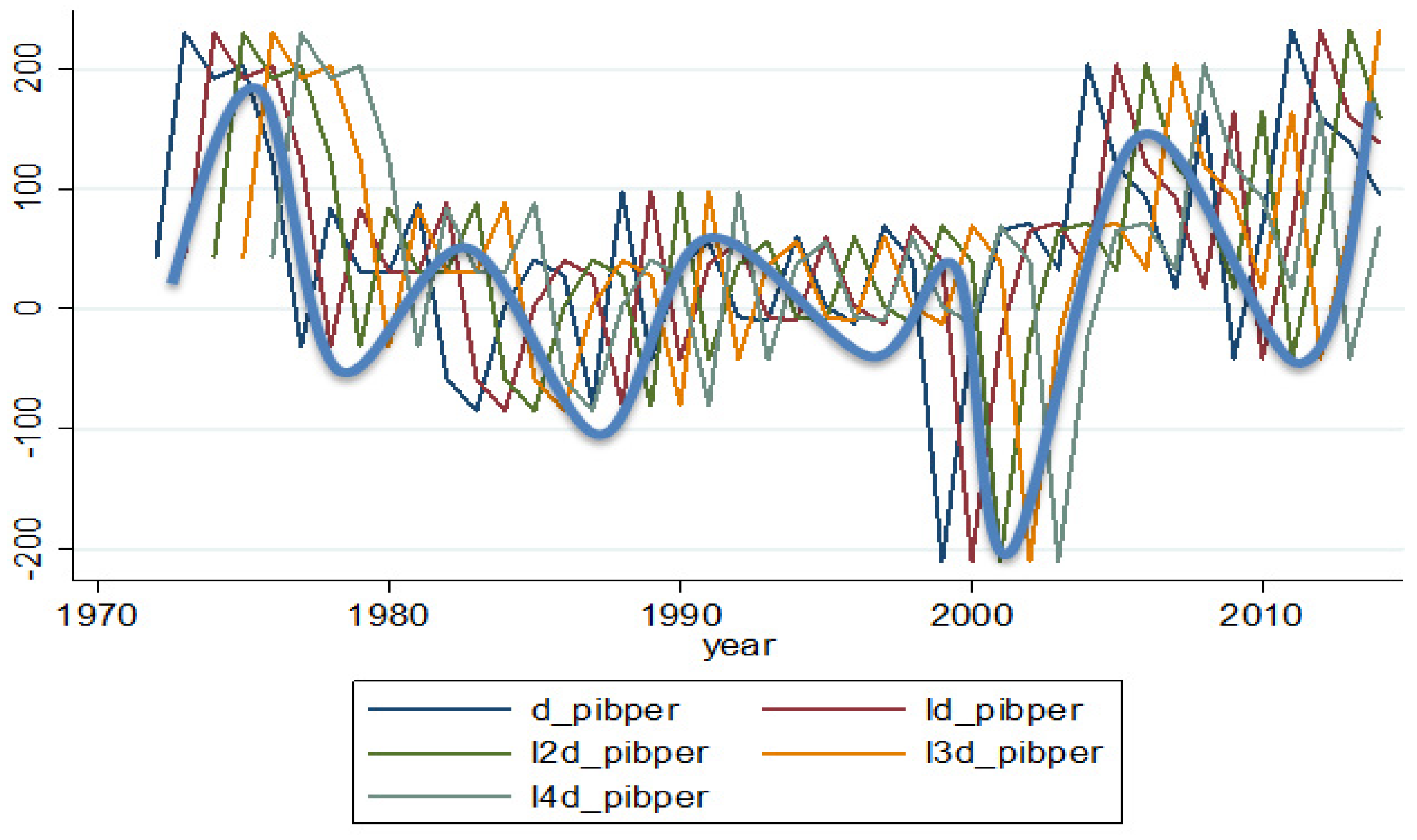
When plotting the lags of the GDP per capita together, a cyclical behavior is visible—the same that allows one to intuit that the structure of the lags does not necessarily have to be linear—and indicates that it is possible to adopt various techniques or methodologies, such as the suggestion of this investigation. It also indicates that, for research, it is advisable to perform a third degree Almon polynomial given movements similar to a cubic or a third-degree curve (see Figure 1).

Almon Polynomial Estimation

To illustrate the estimated results (

Table 2. Almon polynomial method estimates.

Estimation	$\propto$	z0	Z1	Z2	Z3
Coefficients	−1.14	0.0006	−0.0083	−0.00094	0.000736
Value (t)	−3.36	0.73	−0.77	−0.73	0.91
R squared	0.699 = 70%
Value(F)	20.94

Source: World Bank 2015. Elaboration: the authors through the program Eviews.

), Equation (3) is used. This equation shows the values of the following lags (Z):

$$Y_t=-1.14+0.00060Z_{0t}-0.00829Z_{1t}-0.000941Z_{2t}+0.000736Z_{3t}+{\mu }_t$$

In turn, Equation (2) is used to show the value of the coefficients obtained in the estimate.

$${\beta }_0=a_0=-0.00025$$

$${\beta }_1=a_0+a_1+a_2=0.00060{\beta }_2=a_0+2a_1+4a_2=-0.00043$$

$${\beta }_3=a_0+3a_1+9a_2=0.00107$$

By substituting the values in the general equations, we obtain the present equation:

$$Y_t=\propto +{\beta }_0{X}_{t-1}+{\beta }_1{X}_{t-2}+{\beta }_3{X}_{t-3}+{\mu }_t$$

$$Y_t=-0.00025+0.00060X_t-0.00043X_{t-1}-0.00107X_{t-2}+{\mu }_t$$

The equation shows a positive relationship, which demonstrates that the Kuznets Environmental Curve hypothesis was met for Ecuador in the 1971–2015 period and that the effect that economic growth had on the environment was significant and fulfilled in a short term. Although the relation of the signs was maintained over time, the parameters of the lags did not contribute significant values for this model, as they were reduced when analyzing the past years. Likewise, the movements of economic growth indicate that the volumes of pollution did not necessarily have a secular tendency but that they moved at the rate imposed by economic growth.

The empirical evidence generated through dynamic models, specifically the Almon polynomial, categorically reveals that there is a direct, positive relationship (mainly in the short term) between economic growth and the increase in the volume of CO₂. The tests performed on the variables and their behaviors allowed us to conclude that, for the analysis of the impact of economic growth on the environment, a third degree Almon Polynomial needed to be carried out with three lags in time. Finally, we tested the causality of the variables using the Granger causality test as follows (

Table 3. Granger causality test results.

Dependent Variable: CO2
Excluded	Chi-sq	Degree of Freedom	Prob.
GDP per capita	9.686993	2	0.0079
All	9.686993	2	0.0079
Dependent variable: GDP per capita
Excluded	Chi-sq	Degree of freedom	Prob.
CO2	0.272962	2	0.8724
All	0.272962	2	0.8724

$H_O=Prob.<5\%->SignificativaoPrecedente$

).

This methodology reveals whether one variable is caused or precedes the other through the probability of significance of the model, which decrees that, since said probability of less than 5% is significant and precedes another variable, the model dependent variable is CO₂ because the probability of GDP per capita proves to be significant, that is, it explains CO₂ emissions.

In the case of the VAR model, the equation shows that the block of the lagged values of economic growth helps to improve the forecast of CO₂ emissions generated by the model, that is, that the lags of growth temporarily precede the present values of the emissions of CO₂.

5. Discussion

Economic growth is usually enacted as a synonym for social and individual well-being in a globalized and Westernized world, becoming an idealized goal for nations that are mired in inequality and poverty. According to [38], when analyzing nine South American countries located in a region composed of developing countries, it was shown that Bolivia, Brazil, Chile, Colombia, Ecuador, Peru, Paraguay, Uruguay, and Venezuela presented a positive relationship between economic growth and environmental deterioration in seven of the nine study countries during the period 2000–2012.

The greatest increases in CO₂ emissions were found in Brazil and Chile with increases that remain between 0.04 and 0.12 metric tons per year and whose trends show that these levels could continue to grow over time. On the other hand, it can be observed that Venezuela and Paraguay showed no significant correlations, indicating a case that moves away from the traditional ECK postulate. This allows one to deduce that, in the developing countries, the Kuznets Environmental Curve hypothesis does not have a high efficiency level since the progress of underdeveloped countries does not allow them to use their knowledge potential to take advantage of the exploitation of their natural resources for the purpose of satisfaction, development, growth, and success or to be able to replace the environmental deterioration caused by such exploitation.

The eagerness for economic growth has inevitably increased the consumption of natural resources and the pressure to protect the environment. South America is a palpable case of environmental deterioration in support of economic activity [39]. In the general model presented for Latin America, CO₂ levels began to increase from US $4500 GDP per capita. Brazil, Colombia, and Peru were identified as the countries with the highest pollution growth between 1980 and 2000, maintaining this trend for Brazil in the years of study proposed in this research and including Chile in the analysis. As with some developing countries in Africa and Asia, the problems in the South American region could lead to failure in environmental policies and the commitment to conscious environmental management, with problems that could be extended to other indicators of environmental deterioration, such as deforestation and the emission of other pollutants [40].

As [41] establishes in the time series regression analysis, when the regression model includes lagged values of the explanatory variables in addition to current values, it is called the distributed lag model. This is a method that was applied in this work, and it was selected due to the approach of Shirley Almon. As Gámez (2010) mentions, it is a technique that allows the coefficients of the explanatory variables to be represented by more flexible functions, allowing a developed understanding of their effects.

The study of the environmental pollution generated by the CO₂ emissions that come from the industrialization processes of countries is crucial because it opens an opportunity to discuss what is most important in an economy. Is it economic growth despite the environmental deterioration? There is a wide and diverse range of literature in this regard, and all positions have important contributions to the subject, but there is no exact definition. The research work presented in this document was based on this discussion.

The estimate made in lags of one period yielded positive results in terms of expected signs, econometric tests, and functional form, but the results that were found to be different in the relationship were considerable, since they were reversed when returning two or more periods in time. This indicates that, in Ecuador, the relationship of the Kuznets Environmental Curve hypothesis exists in the short term.

In Ecuador, during the last few years, the national government has shown interest in the care of the environment through decrees, legislation, new regulations, and projects, but above all, emphasis on compliance, evaluation, and monitoring of each proposed activity has been observed. At the same time, it is understood that there are still no specific regulations for pollutants, a situation that should change in the medium term.

The dilemma that is generated in this relationship is not easy to handle because people want their needs to be met and only perceive what happens to them in the short term, thus little time is devoted to reflecting about the consequences of their lifestyles if the amount of CO₂ produced has a positive trend in the long term. This decision is one of the great predicaments that governments face—what is the best for the people?

The relationship between economic growth and environmental deterioration and its effects requires the government to worry about knowing the best solution and whether to drop the GDP to obtain the same effect on CO₂ emissions or to take measures to reduce the impact of emissions. Given this situation, the government must be concerned with making decisions for the resolution of conflicts arising from environmental management within both the scope of the national government and the community itself.

Currently, priority has not been given to the economic policy of environmental management—which has become notorious—hence the low presence of proposals in the local government and an increase in metric tons per capita of CO₂ emissions throughout the study period, for example, in 1977 (1015), 1984 (2409), 1994 (1219), 2000 (1641), and 2014 (2762) according to the World Bank 2015 database. In order to ensure environmental elements as an essential part of natural, cultural, and economic capital, the Ecuadorian government has to appeal to implement an environmental policy that interrelates and reconciles economic, socio-cultural, and environmental aspects to create and/or improve participation mechanisms for environmental management so that this participation occurs from the beginning of the consideration of an idea and not only when society feels affected, in accordance with the principle of prevention of environmental conflicts.

6. Conclusions

The results of the present investigation show that the Kuznets Environmental Curve hypothesis for the Ecuadorian case through ad-hoc estimates demonstrates the relationship between economic growth and environmental degradation in the short term. Thus, Ecuador, being a developing country, is forced to exploit their natural resources until they reach a level of satisfaction where they can use these resources to develop economically, technologically, etc. The knowledge of this exploitation of resources, which shows varying behaviors throughout the analysis period and generates environmental pollution with recognizable implications, allows the country with new knowledge to be able to counteract such contamination by implementing technological innovation and environmental education.