Unit-Based Emissions Inventory for Electric Power Systems in Kuwait: Current Status and Future Predictions

Abstract

Obtaining accurate estimates of emissions from electric power systems is essential for predicting air quality and evaluating the effectiveness of any future control technologies. This paper aimed to develop unit-based emissions inventories for electric power systems in Kuwait using different parameters, including fuel specifications and consumption, combustion technology and its efficiency, unit capacity, and boiler type. The study also estimated the future emissions of NOx, SO₂, CO, CO₂, and PM₁₀ up to the year 2030 using a multivariate regression model in addition to predicting future energy demand. The results showed that annual (2010–2015) emissions of all air pollutants, excluding SO₂ and PM₁₀, increased over the study period. CO had the greatest increase of 41.9%, whereas SO₂ levels decreased the most by 13% over the 2010 levels, due to the replacement of heavy fuel oil. Energy consumption in 2015 stood at approximately 86 PJ, with natural gas, gas oil, crude oil, and heavy fuel oil making up 51.2%, 10.7%, 3.1%, and 35%, respectively. Energy demand was projected to grow at an annualized rate of 2.8% by 2030 compared to 2015 levels. The required installed capacity to meet this demand was estimated to be approximately 21.8 GW (a 34% increase in capacity compared to 2015 levels). The projected emission rates showed that, of the five air pollutants, SO₂ and PM₁₀ are expected to decrease by 2030 by 34% and 11%, respectively. However, peak monthly emissions of SO₂ would still only be 14% lower compared to the 2015 monthly average. In contrast, emission levels are projected to increase by 34.3%, 54.8%, and 71.8% for CO₂, NOx, and CO, respectively, by 2030 compared to 2015 levels. Accordingly, a more ambitious target of renewables penetration needs to be adopted to reduce emission levels going forward.

1. Introduction

Electric power systems consume significant amounts of fossil fuels in order to reliably generate electricity and meet rising electricity demands. This is associated with significant costs to the environment due to increasing environmental discharges. These discharges include atmospheric pollutants and greenhouse gases resulting from the burning of fossil fuels. Carbon dioxide (CO₂) emissions from electricity generation make up the vast majority of global greenhouse gas emissions [1]. In the United States, for instance, power plants emitted approximately 29% of the total greenhouse gas emissions (the highest recorded contributor to emissions) in 2015 [2], and other researchers trace as much as 63% of cumulative CO₂ emissions in the atmosphere alone to be due to the burning of fossil fuels [3]. Thermal power plants are also responsible for 59% of the total atmospheric sulfur dioxide (SO₂) emissions in the U.S. [4], and 50% of SO₂ emissions in India [5]. In addition, ambient air pollutants impose a serious threat to health and have been linked with adverse health effects that have been widely addressed in the literature [6,7,8,9,10].

In Kuwait, demands on electricity and water more than doubled in 2015 compared to 2000 levels. To meet this significant growth in demand, the power sector relies on cogeneration plants that are fueled exclusively with fossil fuels [11]. Power generation and water desalination systems work simultaneously to produce electricity and desalinate seawater by cogeneration power-desalting plants. Several studies in Kuwait have addressed air quality and have shown results of potentially dangerous levels of some atmospheric pollutants [12,13,14]. For example, Al-Baroud et al. [15] found that the concentrations of oxides of nitrogen (NOx) and SO₂ exceeded the air quality limits set by the Environmental Protection Agency (EPA). A few studies simulated SO₂ emissions from power plants and showed exceedances of SO₂ concentrations compared to the standard limits [16,17,18,19]. Therefore, the Kuwait Environmental Protection Authority (KEPA) has emphasized reducing air pollution and improving air quality.

Recently, the United Nations Development Programme and the state of Kuwait (UNDP Kuwait) have developed the Kuwait Integrated Environmental Management (KIEM) system, which aims to review current environmental regulations and establish new air pollutant standards [20]. Evaluating air quality data is part of the task, and to effectively manage that task, a reliable and updated emissions inventory should be created. However, current air quality standards in Kuwait have failed to reflect emission inventories from energy systems with updated estimates, a hole this paper will ultimately fill. In this paper, an updated unit-based emissions inventory for a period of 6 years (2010–2015) was developed on the basis of unit by unit data and calculations; then, the unit results were grouped by similar combustion technologies. In characterizing temporal or spatial patterns of air quality in Kuwait, most of the previous studies addressing the impact of power plants relied on poorly estimated rates and of only monthly emissions. In contrast, this study analyzed air pollutant emissions on an hourly, daily, and seasonal basis for 2014 and annual basis for 2010 to 2015. From this, a full profile of Kuwait’s power plant emissions can be established.

The paper also aimed to predict future atmospheric emissions using a multivariate regression model through analyzing future energy demand and fuel consumption. In predicting future emissions, different approaches across the globe have been used [21,22,23,24]. Examples include modeling the relationship between economic growth and population with total energy consumption [25], developing an empirical model for estimating greenhouse gas emissions on the basis of sector-specific projected electricity consumption [26], or using historical polynomial trends solely such as [27]. In this study, future emissions were estimated by predicting electric demand for each type of fossil fuel up to 2030, using a multivariate regression model. A similar approach has been adopted by several studies in the literature and is useful for providing a reasonably accurate estimate of future emissions on the basis of historical trends when data on economic output or population growth is harder to estimate moving forward [28,29]. On that basis, the monthly emissions of CO₂, NOx, SO₂, CO, and particulate matter 10 micrometers or less (PM₁₀) are projected and compared on a percent change basis up to 2030. The model for estimating future emissions inventories that is presented in this paper was based on the assumption that the control units that are installed in the future will be similar to those that are currently in use in the respective power plants. Streets and Waldhoff [30] suggest that accounting for emission control units at point of release could reduce the estimated emissions by as much as half the original values. As such, the results of this study mirror a worst-case scenario of the potential emission profile. It is anticipated that predicting future emission trends on the basis of projected fuel specifications and consumption, combustion technology and its efficiency, and other important factors would provide KEPA with meaningful guidance that could aid the development of a strategic action plan to meet its mandate. This will fill an existing gap since the Ministry of Electricity and Water (MEW) 2030 plan for installing new power plants did not address future emissions, whether by combustion technology or fuel source.

2. Methodology

2.1. Electric Power Infrastructure Specifications

Kuwait relies on seven power plants for power production, all of which are strategically located in close proximity to seawater, in accordance with the cogeneration technologies used in those power plants to simultaneously desalinate seawater. The installed capacity at each of those power plants can be found in [31].

The process of obtaining the hourly fuel consumption rates is explained as follows. The monthly fuel consumption data at each power station in Kuwait are collected from the MEW [11]. The MEW provided spreadsheets that further dissect the monthly data into daily operational consumptions that are not only power plant-specific but also turbine-specific. Thus, the hourly electricity production rates were obtained through Kuwait’s National Command Center (NCC), which allocates electricity needs throughout Kuwait’s electricity network. The problem with the hourly rates obtained through the NCC is that the data were rounded off to the nearest 10th for every hour. Hence, the daily totals of electricity production reported by the NCC were not necessarily in agreement with the totals reported by the power plants. This necessitated normalization before the NCC data could be of any use. The NCC values were normalized using the MEW daily spreadsheets so that the hourly totals would be in agreement.

A result of the normalization process was an hourly factor of how much electricity was produced at each hour for each day of 2014. Because electricity production is coupled with fuel consumption, those hourly factors were used to generate hourly fuel consumption rates by using the daily fuel consumption rates reported by the MEW. The fuel consumption data were then converted to British thermal units (BTUs) to facilitate the evaluation of the emission rates using emission factors.

Table 1. Seasonally averaged calorific values for natural gas (NG), gas oil (GO), crude oil (CO), and heavy fuel oil (HFO).

Fuel	Summer	Autumn	Winter	Spring
Natural gas (MMBtu/MSCF)	1.071	1.071	1.071	1.071
Gas oil (MMBtu/BBL)	5.425	5.405	5.418	5.412
Crude oil (MMBtu/BBL)	5.480	5.480	5.480	5.480
Heavy fuel oil (MMBtu/BBL)	5.607	5.573	5.446	5.587

shows the calorific values used in this study. These values were obtained from the fuel provider, which is the Kuwait National Petroleum Company (KNPC). Detailed information about the fuel consumption data can be found in [32].

2.2. Mathematical Model

The emission factors were obtained through the AP-42 for the respective pollutants and their corresponding combustion mechanisms [33]. The selected pollutants for this analysis were CO₂, NOx, SO₂, CO, and total PM. Sulfur content of the respective fuel is a key factor for determining the SO₂ emission level. The only sort of end-of-pipe treatment available across power plants in Kuwait is the desulfurization of liquid fuel prior to consumption for power production, or the operational switch between steam and gas turbines to increase fuel efficiency. The desulfurization pre-treatment is reflected in the sulfur content values used for calculating emission factors for air pollutants and the operational switch is reflected in the fuel consumption data. Hence,

Table 2. Sulfur content of fuels (weight %).

Fuel	Summer	Autumn	Winter	Spring
Natural gas	0.0267	0.0200	0.0433	0.0172
Gas oil	0.156	0.158	0.145	0.225
Crude oil	2.645	2.645	2.645	2.645
Heavy fuel oil	3.69	3.88	3.76	3.79

outlines the seasonally averaged sulfur content for each type of fuel used in power stations in Kuwait [11].

In addition, NOx emissions flow rates were estimated for steam and gas turbines assuming operation under high load conditions.

Table 3. Emission factors due to combustion of fuels in steam turbines (ST) and gas turbines (GT) in kg/MMBTU. NOx: Oxides of nitrogen.

	NG		GO		CO	HFO
Pollutant	ST	GT	ST	GT	ST	ST
CO2	49.2	49.9	58.9	71.2	65.2	61.6
NOx	7.78 × 10−2	0.145	6.33 × 10−2	0.399	0.123	0.121
SO2	2.46 × 10−4	1.08 × 10−2	6.40 × 10−2	7.83 × 10−2	1.03	1.52
CO	3.44 × 10−2	3.72 × 10−2	1.32 × 10−2	1.49 × 10−3	1.3 × 10−2	1.28 × 10−2
PM	3.11 × 10−3	2.99 × 10−3	5.28 × 10−3	5.44 × 10−3	1.82 × 10−2	2.55 × 10−2

outlines the monthly averaged emission factors as per the respective combustion technology and fuel for 2014.

Accordingly, the hourly emission rates for all air pollutants were calculated using Equations (1) and (2) for steam and gas turbines, which were based on the AP-42 [33] and expanded to fit for the energy production system in Kuwait.

$$\begin{array}{l}ER\left(\frac{kg P}{steam turbine unit i . hour}\right)\\ =M_{NG-i}\left(\frac{MMBtu}{hour}\right)\ast E{F}_{ST-NG-P}\left(\frac{kg P}{MMBtu}\right)+M_{GO-i}\left(\frac{MMBtu}{hour}\right)\\ \ast E{F}_{ST-GO-P}\left(\frac{kg P}{MMBtu}\right)+M_{FO-i}\left(\frac{MMBtu}{hour}\right)\ast E{F}_{ST-FO-P}\left(\frac{kg P}{MMBtu}\right)\\ +M_{HFO-i}\left(\frac{MMBtu}{hour}\right)\ast E{F}_{ST-HFO-P}\left(\frac{kg P}{MMBtu}\right),\end{array}$$

(1)

$$\begin{array}{l}ER\left(\frac{kg P}{gas turbine unit j . hour}\right)=M_{NG-j}\left(\frac{MMBtu}{hour}\right)\ast E{F}_{GT-NG-P}\left(\frac{kg P}{MMBtu}\right)+M_{GO-j}\left(\frac{MMBtu}{hour}\right)\ast \\ E{F}_{GT-GO-P}\left(\frac{kg P}{MMBtu}\right),\end{array}$$

(2)

where $ER$ is the hourly emission rate per unit for air pollutant $P$, $M$ is the fuel consumption rate, and $E$ is the corresponding emission factor for every fuel per consumption technology. The emission factors used in the equations were readily estimated to reflect all the changes in calorific values, as well as sulfur content to unify the units for easier interpretability and the facilitation of comparison between different fuels.

2.3. Predictive Model

For the emission factor corresponding to every type of fuel-powered technology at power plants, in addition to the fuel consumption rates at those units, the emission rates were evaluated and used to estimate the hourly emissions. These were summed over the required time period for every power plant’s fuel powered technology because the analysis was focused on the temporal and not spatial patterns associated with current emissions.

A multivariate linear regression model was used for estimating future energy consumption, as well as the monthly emission rates of CO₂, NOx, SO₂, CO, and total PM based on monthly data covering a 6 year period from 2010 to 2015, as shown in Equation (3). This was a general form of the multivariate regression model used for the six developed models, where Ex corresponded to the monthly energy demand in PJ or the monthly emission rate in tons, depending on the input parameters. Moreover, using historically averaged efficiencies, the corresponding electricity consumption rates were calculated, on the basis of which the required electricity production capacity was estimated and compared to the MEW’s plan for installing newer units.

Each data point was characterized with 13 features. The first feature (a) corresponded to a ‘continuity’ parameter reflecting how far in time (# of months) a data point was with respect to the first data point. Every other feature was considered a flag parameter (0 or 1) corresponding to the month (X_i) of the year to account for the energy consumption seasonality observed in Kuwait. In addition, “I” was the intercept term associated with the linear regression.

This model structure was chosen because of the apparent seasonality in the energy consumption profile of Kuwait highlighted in [31], on the basis of which a reasonably accurate model that accounted solely for the monthly seasonality would suffice. In addition, relying on other parameters for estimating the future emissions or energy demand such as population growth, growth domestic product, or electricity unit cost would only add to the uncertainty of future predictions because those values would have to be predicted in their own rights due to the absence of proper data reflecting their future outlook, unlike other studies such as [25,26,27]. The seasonality assumption worked rather well in predicting future emissions, as reflected by the reasonably good R² values obtained and outlined in

Table 4. Regression parameters for multivariate models.

	Energy Demand in PJ	CO2 in Tons	NOx in Tons	SO2 in Tons	CO in Tons	PM in Tons
R2	0.94	0.91	0.73	0.71	0.95	0.83
I	37.04	3697.4	34212.6	678.3	638.6	3697.4
ao	0.17	32.8	−61.1	6.3	−0.4	32.8
a1	0.90	671.8	−947.9	−30.4	−11.4	671.8
a2	−4.29	−55.6	−5911.2	−106.1	−103.5	−55.6
a3	5.74	1862.6	850.7	32.4	34.1	1862.6
a4	15.99	3823.6	703.7	300.0	62.1	3823.6
a5	24.43	4014.5	5303.4	578.4	146.8	4014.5
a6	30.39	5206.2	10,378.8	638.6	241.7	5206.2
a7	35.89	6137.6	12,204.7	761.5	286.4	6137.6
a8	36.33	6247.1	11,085.3	779.5	271.4	6247.1
a9	28.96	5034.9	6322.6	660.0	176.9	5034.9
a10	18.85	3127.8	886.8	525.1	68.1	3127.8
a11	3.46	904.5	−1025.7	81.7	−5.4	904.5
a12	0.00	0.0	0.0	0.0	0.0	0.0

.

$$E_X=I+a\mathfrak{o}\ast X_0+{\sum }_{i=1}^{12}{a}_i\ast X_i.$$

(3)

The regression parameters associated with all six models are shown in Table 4, along with the respective R², which showed reasonable accuracy for the purposes of this study. Concretely, energy demand, CO₂ emissions, and CO emissions seemed to follow seasonality to a reasonable level of accuracy. However, the reason the model was less accurate in predicting NOx emissions was primarily due to gas oil consumption being an operational decision and not necessarily following a seasonal pattern, unlike other fuels, because it is consumed primarily for the purpose of gradually achieving specific operational conditions in between changing fuels. Similarly, the reason the model’s accuracy was lower in predicting SO₂ and PM emissions was because of the fast-paced reduction in crude oil consumption over the period of the input data, which does not necessarily follow a seasonal pattern as well.

3. Results and Discussion

The first section of this analysis discusses the temporal patterns associated with emissions of CO₂, NOx, SO₂, CO, and PM₁₀ for 2014. This section is divided into three subsections, the first of which analyzes the daily emissions of those pollutants for 2014, and the second subsection discusses the general trends in annual emissions due to power plants in Kuwait spanning a period of 6 years from 2010 to 2015. The third subsection performs a seasonal hourly analysis on the days with the respective highest emissions for each air pollutant.

3.1. Current Temporal State of Emissions

Daily Emissions for 2014

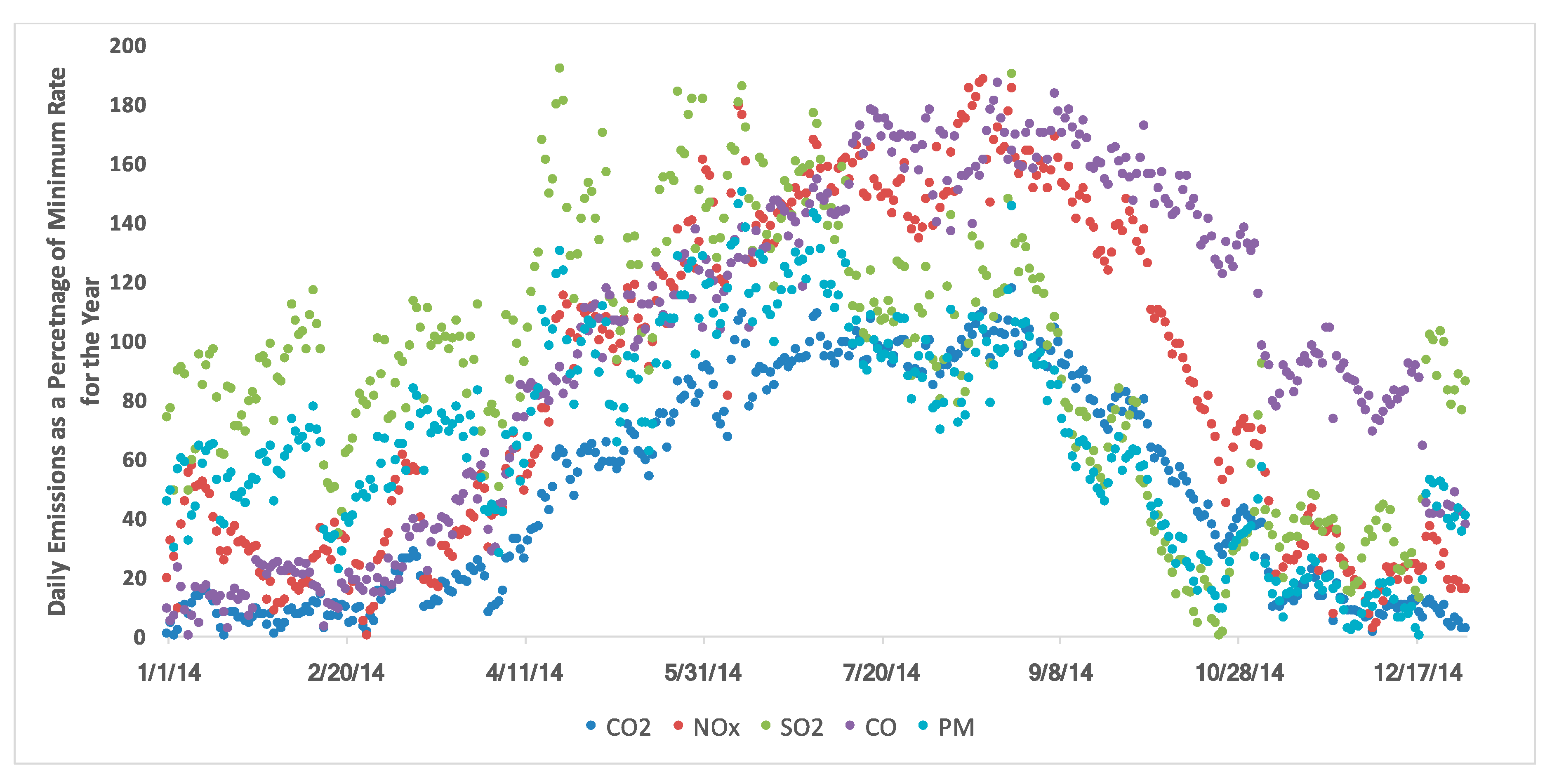
Figure 1 shows the daily emissions for CO₂, NOx, SO₂, CO, and PM₁₀ in 2014 as a percentage of the respective daily emissions rate. The most notable distinction between the five profiles is that all of them seemed to start and end the year at approximately the same level, except for CO, which was significantly higher at the end of the year because of the relatively higher natural gas consumption by year end. Otherwise, they all peaked during the summer, when fuel consumption and electricity load are highest.

CO₂ daily emission rate peaked at the end of August. The highest observed daily emission rate for CO₂ was approximately 160,000 tons per day, whereas the lowest was approximately 80,000 tons (half of the highest rate) at the beginning and the end of the year.

Similarly, NOx daily emission rate peaked at approximately the same period (end of August) at 412 tons per year. It started the year (and ended) at a rate of approximately 170 tons per day, which more than doubled to reach the maximum during summer. This great discrepancy between the lowest and highest emission rates indicate how sensitive Kuwait’s power production systems are in handling the increased electrical load during the summer.

The highest emission rate for SO₂ stood at approximately 1700 tons per day, whereas the lowest observed daily emission rate was 1000 tons per day at the beginning as well as end of the year. The highest SO₂ daily emission rate occurred in the spring season and not in the usual summer season.

The CO profile showed a somewhat different trend, peaking at 65 tons per day during the summer but with a 25% increase for the end of year emission rate over that for the beginning of year. The starting daily emission rate was 24 tons per day, and the year ended with a daily emission rate of 30 tons per day, which was due to the significant increase in gas oil consumption recorded for 2014.

Finally, the total PM daily emission rate showed a peak value at the beginning of June at approximately 33 tons per day. The rate started at 20 tons per day and ended the year at approximately the same value, with the usual peak during summer time.

3.2. Seasonal Analysis of Emission Levels for 2014

Hourly emission rates are not continually recorded by KEPA or by the power plants that are responsible for releasing them into the atmosphere. Accordingly, in preparing the results of this analysis, a database containing the hourly emission rates of different air pollutants was produced, which was further expanded to facilitate the study of the power production system in Kuwait.

The base case analysis was conducted on a seasonal basis, where the day with the highest emissions for the respective air pollutant for each season was studied on an hourly basis to represent the worst-case scenario. This was done to investigate the limits of the system at peak load of emissions. In addition, the daily loads were divided into steam and gas turbine contributions to determine their contributions to the total emissions.

• Base case (C1—Highest emissions): refers to the worst-case scenario, which represents emissions of the days with the highest emissions for each season.
• Case 2 (C2—Highest electrical load): represents emissions of the days with the highest electrical loads of each season.
• Case 3 (C3—Highest fuel consumption): represents emissions of the days with highest fuel consumptions for each season.

This could explain some of the trends seen in the seasonal analysis of hourly emission rates with respect to the type of fuel that is contributing to emissions in addition to highlighting the variability in how emission levels change under the three cases.

3.2.1. Seasonal Analysis of Daily Emissions by Respective Highest Rate (C1)

In this section, the day with the highest emissions for the respective air pollutant for each season is studied on an hourly basis to represent the worst-case scenario. The hourly bars are further dissected to indicate the fuel source of the air pollutant. The summer season comprised the months of June, July, and August. Autumn followed, with September, October, and November. December, January, and February counted towards the winter season. Finally, the spring season comprised the months of March, April, and May.

Carbon Dioxide

The general overview of the CO₂ emission profile (see Appendix A Figure A1) showed a peak during the summer and a minimum during winter. The highest days with CO₂ emissions for summer, autumn, winter, and spring were the 26 August, 7 September, 11 January, and 31 May, respectively. During the summer, autumn, and spring seasons, the peak load was observed at approximately 14:00, whereas the minimum rate was observed at approximately 6:00. In contrast, for the winter season, a peak load was observed at approximately 18:00, whereas the minimum load was observed at 4:00. The highest hourly emission rate stood at 7,000,000 kg per hour, which was more than double the minimum rate of 2,700,000 kg per hour. Natural gas proved to be the most significant source of CO₂ emissions throughout all seasons except for spring, when the CO₂ emissions due to heavy fuel oil were comparable with those due to natural gas.

Even though natural gas was the highest contributor to CO₂ emissions, Figure 2C1 indicates that the steam turbines always contributed to higher emission rates than gas turbines. This was demonstrated by the fact that natural gas was not strictly consumed by gas turbines, but a significant amount was consumed by steam turbines. Accordingly, the highest daily emission rate of CO₂ was that on 26 August at 160,000 tons/day, of which 100,000 tons/day were due to steam turbines emissions. For the lowest emission rate on 11 January, it stood at 83,000 tons/day, of which 63,000 were due to steam turbines.

Oxides of Nitrogen

Similar to the above general trend observed for CO₂, the same could be seen for NOx (see Appendix A Figure A2). The striking difference between the two pollutants was the fact that gas oil contributed to as much as 35% of the hourly emission rate. In a very close second place came natural gas, which caused approximately 33% of the NOx emissions. This highlighted the fact that even though gas oil is the cleanest of the liquid fuels, it is still a major source for NOx. The highest days with NOx emissions for summer, autumn, winter, and spring were the 18 August, 7 September, 8 January, and 31 May, respectively. It is worth noting that during autumn and spring, the same two days with the highest CO₂ emissions were also those with the highest NOx emissions. The highest NOx hourly emission rate was estimated at approximately 18,000 kg/hr, which represented a 125% increase over the minimum emission rate (8000 kg/hr).

Consequently, gas turbines were the main source of NOx emissions for all seasons (see Appendix A Figure A2). The highest daily emission rate was found to be approximately 412 tons/day on 18 August, where gas turbines played part in as much as 240 tons/day. Moreover, the lowest daily emission rate occurred on 8 January at 230 tons/day, of which 120 tons were due to gas turbines.

Sulfur Dioxide

The same exact general profile was observed for SO₂ (see Appendix A Figure A3) as those observed for the previous two pollutants. All pollutants peaked during the same hours of the day in their respective seasons. Because SO₂ is released by the combustion of sulfur-containing fossil fuels, one expects crude oil and heavy fuel oil (fuels with highest sulfur contents) to be the major sources of SO₂ emissions. Yet, through the winter and spring seasons, heavy fuel oil seemed to be the exclusive source of SO₂ emissions, the reason being that no crude oil was consumed during those days with the highest SO₂ emissions. The highest days with SO₂ emissions for summer, autumn, winter, and spring were the 26 August, 3 September, 11 February, and 21 April. The highest hourly rate stood at approximately 78,000 kg/hr, whereas the lowest rate was 40,000 kg/hr.

In addition, steam turbines entirely dominated gas turbines in SO₂ emissions during all seasons (Figure 2C1). The maximum daily emission in the summer season (26 August) reached 1700 tons of SO₂ per day. For the lowest daily emission rate on 11 February, it stood at approximately 1150 tons/day.

Carbon Monoxide

The same overall profile could be observed for CO as well for peak and minimum hours during all seasons (see Appendix A Figure A4). In contrast, natural gas dominated contributions at all seasons, producing as much as 83% of the total CO emissions. The other two fuels causing the rest of the emissions were heavy fuel oil and crude oil, both contributing equally for all seasons except for winter, when heavy fuel oil dominated crude oil. The highest days with CO emissions for summer, autumn, winter, and spring were 22 August, 7 September, 15 December, and 29 May, respectively. The lowest hourly rate of CO occurred during winter at 1500 kg/hr, which was half of the computed maximum of 3000 kg/hr.

However, although natural gas accounted for over 80% of CO emissions, those emissions stemmed mainly from steam turbines (Figure 2C1). This highlights the earlier observation that steam turbines contributed as much as gas turbines (if not more than) to natural gas combustion. The highest daily CO emission was 64 tons/day, which occurred on 22 August, to which steam turbines contributed 37 tons/day.

Total Particulate Matter

The general trend observed for total PM regarding the peak load and minimum hours of the day was analogous to what was established from investigating the other pollutants (Figure A5). The largest source of PM emission was heavy fuel oil, accounting for as much as 92% (during spring). Heavy fuel oil was the dominant source of PM because it contains various chemicals and metals. The other two fuels that made significant contributions to PM emissions were crude oil and natural gas. During the summer and autumn seasons, the crude oil contribution reached as much as 25% of the total PM emissions. The highest days with PM emissions for summer, autumn, winter, and spring were the 11 June, 3 September, 11 February, and 21 April, respectively. It is worth noting that two of those days (all but 11 June) correlated with the same days when the highest SO₂ emissions were observed because of the strong and apparent reliance of PM and SO₂ emissions on heavy fuel oil. The highest hourly emission rate of PM was estimated at approximately 1600 kg/hr, whereas the lowest was 800 kg/hr.

Thus, Figure 2C1 indicates that steam turbine emissions completely dominated those by gas turbines. The highest daily emission rate occurred in the summer (11 June) at 34 tons/day, of which 30 tons/day were due to steam turbines. Furthermore, the lowest daily emission rate, which occurred during the winter season (11 February) stood at 23 tons/day, of which 22 tons/day were contributed by steam turbines.

3.2.2. Seasonal Analysis of Daily Emissions by Highest Electrical Load (C2)

In 2014, the days with the highest electrical loads for summer, autumn, winter, and spring were the 2 July, 8 September, 15 December, and 31 May, respectively. Figure 2C2 shows the CO₂ daily emission rates for each of those days. It indicates that steam turbines were the dominant contributor to CO₂ emissions for all seasons, yet the emission rates were lower than for the base case (S1) (i.e., days with highest CO₂ emissions) by as much as 7%. The highest daily emission rate for the summer season stood at just over 152,000 tons/day, whereas the lowest rate that occurred during the winter season was 80,000 tons/day.

In the case of NOx emissions, the results somewhat varied significantly over those of the base case in Figure 2C2. The main difference was observed for the turbines contributing to the emissions. Gas turbines for the base case clearly dominated, whereas for this case, gas turbines showed similar results for only two seasons (autumn and spring). However, for the summer season, gas turbines barely dominated, and for the winter season, steam turbines resulted in more NOx. The highest and lowest emission rates were 380 and 170 tons/day, respectively.

As for SO₂, a significant variation was observed between this case and the base case. The exclusive contributor to SO₂ emissions remained steam turbines, with very little or no contribution from gas turbines. Moreover, the peak emission rates did vary considerably by as much as 53% over the base case. The highest observed daily emission rate of SO₂ was 1580 tons/day, whereas the lowest one was 572 tons/day. Figure 2C2 shows the daily emission rate of SO₂ on high electric load days (C2).

Similarly, the case remains for CO emissions as well. Figure 2C2 shows the daily CO emission rate as per source for the days with the highest electrical loads of each season. The main contributor to CO emissions remained steam turbines in a somewhat similar fashion to the base case. Nonetheless, the highest emission rates varied considerably—as much as 11%. It is worth noting that the maximum daily emission rate for this case was observed during autumn and not summer, as per the base case. The highest daily rate stood at 62 tons/day, whereas the lowest rate was 43 tons/day.

Finally, the general profile for the days with highest PM₁₀ emissions did not deviate much from those of the base case (Figure 2C2). Steam turbines clearly dominated gas turbine emissions of PM₁₀. However, the highest daily rates showed a deviation of as much as 38% from the base case. The highest emission rate for PM₁₀ was approximately 32 tons/day, whereas the lowest was 14 tons/day.

3.2.3. Seasonal Analysis of Daily Emissions by Highest Fuel Consumption (C3)

The days with the highest fuel consumptions were evaluated on the basis of the amount of energy consumed during the respective seasons as a means to normalize the comparison between all types of fuels. In 2014, the days with the highest fuel consumptions for summer, autumn, winter, and spring were 26 August, 7 September, 16 December, and 31 May, respectively. The days with the highest recorded electrical loads and fuel consumptions were the same only for the spring season.

In the case of CO₂, Figure 2C3 shows how the daily emission rates varied per combustion source for the days with highest fuel consumptions in each season. Not much of a deviation was observed for the combustion source, where steam turbines dominated as per the previously established results. Thus, the highest emission rates did not vary as much either, decreasing by a mere 3% over the base case. The highest computed daily rate was 160,000 tons/day, whereas the lowest rate was 76,000 tons/day.

The results differed for NOx (Figure 2C3), yet were somewhat similar to the highest electrical load case. Gas turbines dominated steam turbines as the contribution source, except for the winter season, when steam turbines took the lead. The emission rates differed by as much as 27% over the base case. The highest daily emission rate, which was recorded during the summer season, stood at approximately 408 tons/day. Furthermore, the lowest daily emission rate that occurred in the winter season was 165 tons/day.

SO₂ demonstrated a fairly dissimilar result with those of the base case (Figure 2C3). Steam turbines showed decisive dominance over gas turbines as the combustion source with the highest contribution to SO₂ emissions. The highest daily emission rate stood at 1700 tons/day, whereas the lowest rate was 590 tons/day. A deviation of approximately 55% was observed for the seasonal highest emission rates as per the highest fuel consumption days over the base case.

As for CO (Figure 2C3), emissions due to steam turbines exceeded those due to gas turbines, a result similar to that of the base case. However, the highest daily emission rate was observed during the autumn season and not during the usual summer season, unlike the base case. In addition, the daily rates varied by as much as 13% over the rates observed for the base case. The highest daily emission rate stood at 64 tons/day, whereas the lowest rate was approximately 39 tons/day.

Finally, PM₁₀ results (Figure 2C3) showed a similar trend to the already established results. The main combustion source in this case did not differ from that of the base case; steam turbines were the clear contributor. The highest daily emission rate that occurred during the summer season stood at approximately 33 tons/day. However, the lowest observed rate stood at 14 tons/day, which represented a huge 39% decrease over that of the base case.

From the above, it can be concluded that steam turbines drove the emissions up most, due to outdated installations. Seasonal variations were as high as 55% between peaks, and heavy fuel oil and crude oil were major sources of sulfur dioxide and particulate emissions. Most importantly, the results demonstrated that there was not a common trend for generating electricity in power plants. The days with the highest emissions did not necessarily correspond to the days with the highest fuel consumptions or highest electrical loads. This was due to the variability in fuel allocation being used at each unit. These results lay the ground work for an optimization model based on fuel allocation as a mitigation strategy to reduce the environmental impacts of the energy system.

3.3. Annual Emissions from 2010 to 2015

This section outlines the general trends in annual emissions as shown in

Table 5. Annual NOx, SO₂, CO, and PM₁₀ emissions in 2010 in thousand tons, and the percentages of changes from 2011 to 2015.

Air Pollutant	2010 (Thousand Tons)	2011 (%)	2012 (%)	2013 (%)	2014 (%)	2015 (%)
CO2	36,500	3.6	5.6	4.1	9.7	19.6
NOx	85.3	5.2	10.4	6.9	15.3	35.7
SO2	459.8	−7.8	−11.3	−5.1	−10.9	−13.0
CO	12.9	9.5	15.3	13.9	29.3	41.9
PM10	9.0	−4.4	−6.9	−0.7	−8.5	−2.3

, essentially providing researchers with reasonably accurate estimates of how the power production system in Kuwait contributes to atmospheric emissions of different air pollutants.

In addition, it will serve as input in terms of the monthly emission levels to the regression model in order to predict future emissions. The outlined emissions spanned a period of 6 years from 2010 to 2015. CO₂ emissions for 2015 were approximately 44,000 thousand tons, which represented a 19.6% increase over the initial 36,000 thousand tons released in 2010. In addition, due to the increase in natural gas and gas oil consumption during the study period, the NOx emissions increased considerably. The NOx emissions stood at approximately 116 thousand tons for 2015, which represented a 36% increase over the study period (compared to 2010 levels). This percentage increase represented the second highest among all other pollutants over the same period. The increased reliance on natural gas and gas oil for energy production did not contribute to an increase in NOx emissions alone, but also to CO. The emissions of CO showed the most significant increase in emissions during the study period at 42%. For 2010 and 2015, CO emissions were 12.8 and 18.2 thousand tons, respectively. In contrast, SO₂ emissions experienced the highest decrease at 12%. This decrease was due to the reduction in consumption of crude oil for electrical generation purposes. Emissions of SO₂ stood at 400 and 460 thousand tons for 2015 and 2010, respectively. The only pollutant that showed relatively little variation in emissions throughout the period of 2010 to 2015 was PM₁₀. PM₁₀ emissions were 9.0 and 8.8 thousand tons for 2010 and 2015, respectively.

3.4. Future Predictions of Energy Demand and Emission Rates

The projected rates were consistent with the MEW’s plan of expanding current energy production infrastructure projects on the basis of the historical rates of changes in the consumption of specific fuels and total growth rates of energy demands.

3.4.1. Projected Energy Demand

Energy demand is expected to increase by an average of 2.8% per year by 2030 compared to 2015 levels, yielding a total increase of 41.6% if the observable trend over the prior 6 years is maintained. Total energy demand for 2015 was approximately 806.35 PJ (MEW, 2015). Figure 3 shows the monthly energy demand for 2010–2030, where the dashed lines indicate the forecasted levels. The maximum energy demand in 2015 occurred in August at approximately 86 PJ for the month, which increased to 115 PJ by August 2030 (a 33.7% increase). A valuable insight the projected energy demand could provide is an estimate of the required installed capacity that would meet this demand over time. The second axis of Figure 3 shows the utilized power production capacity over the same period based on historically averaged efficiencies per fuel consumption technology. Accordingly, for a worst-case situation where this demand would entirely be met by fossil fuel burning power plants, the maximum utilized monthly capacity for power production by 2030 would be approximately 17.2 GW. Thus, the required installed capacity to be able to achieve that consumption level based on a historically average utilization rate of 79.1% would be 17.2 GW divided by 0.791, which is approximately 21.8 GW. Concretely, it can be safely assumed that planning for an installed capacity higher than 21.8 GW by 2030 would allow the Ministry of Electricity and Water to meet the required energy demand by then.

As to what the energy mix profile could look like by 2030, one could only look to historical fuel consumption levels for insight. Figure 4 shows the annual historical fuel consumption rates of natural gas, gas oil, crude oil, and heavy fuel oil from 2010 to 2015. Gas oil consumption grew the most (77%) by 2015 compared to 2010 levels, effectively constituting 11.4% of the energy mix by 2015 compared to 7.81% in 2010. Similarly, natural gas consumption rose by 64.1% from 250 PJ in 2010 to 410 PJ by 2015. However, a significant shift in the dynamics of the energy mix occurred in 2015 compared to 2010. In 2010, heavy fuel oil was the main component of the energy mix at 39% compared to natural gas’s share of 37%. However, by 2015, the share of natural gas grew significantly to become 51% of the energy mix compared to a lower 34.2% for heavy fuel oil. However, heavy fuel oil consumption grew by 6.42% over the 6 year period. This was marked by the installation of new gas turbines at several power plants over the course of past years. In contrast, crude oil consumption dropped significantly in 2015 (73%) compared to 2010 levels. This resulted in a lower share of crude oil in the energy mix, dropping from 15.6% in 2010 to only 3.5% in 2015. Accordingly, the energy mix is expected to include natural gas and gas oil at even larger penetration rates by 2030. However, crude oil consumption will most likely disappear from the energy mix sometime around 2025 at that rate. However, the reduction in heavy fuel oil consumption will be limited by the number of dismantled steam turbine units that can only consume heavy fuel oil. Heavy fuel oil share would most likely be replaced by renewable energy, for which the MEW in Kuwait has a target of 15% penetration in installed capacity by 2030.

3.4.2. Projected Emissions

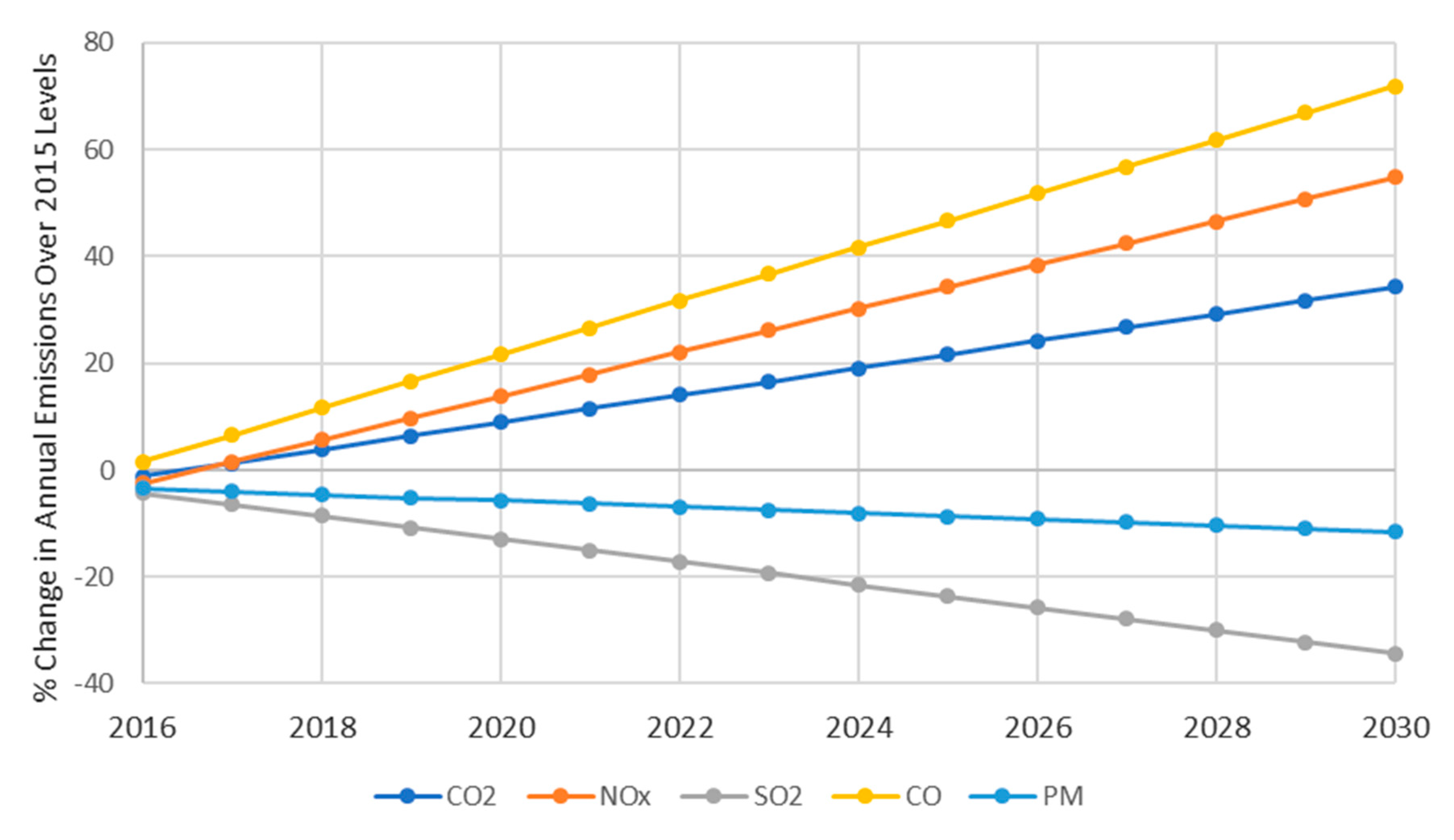
The projected emission levels showed that not all emissions were lower as per Figure 5, which shows the annual changes in emission levels throughout the projected period compared to the corresponding 2015 annual levels.

Interestingly, three pollutants will effectively be higher even when green technologies (NG, GO) constitute most of the energy production infrastructure by 2030. This entails that in order to at least maintain 2015 levels going forward in accordance with global environmental regulations, stricter approaches for emissions reduction need to be employed. Although SO₂ emissions decrease throughout the projected period, as crude oil consumption is eliminated, it would be limited to a 34% reduction by 2030 compared to 2015, most likely due to heavy fuel oil being limited by the effort of dismantling older units. Similarly, PM emissions will have decreased by 11.5% by 2030 compared to 2015 levels. Furthermore, the increased NG and GO penetration into the energy production infrastructure will cause CO, NOx, and CO₂ levels to increase by 72%, 55%, and 34%, respectively, by 2030 compared to 2015 levels.

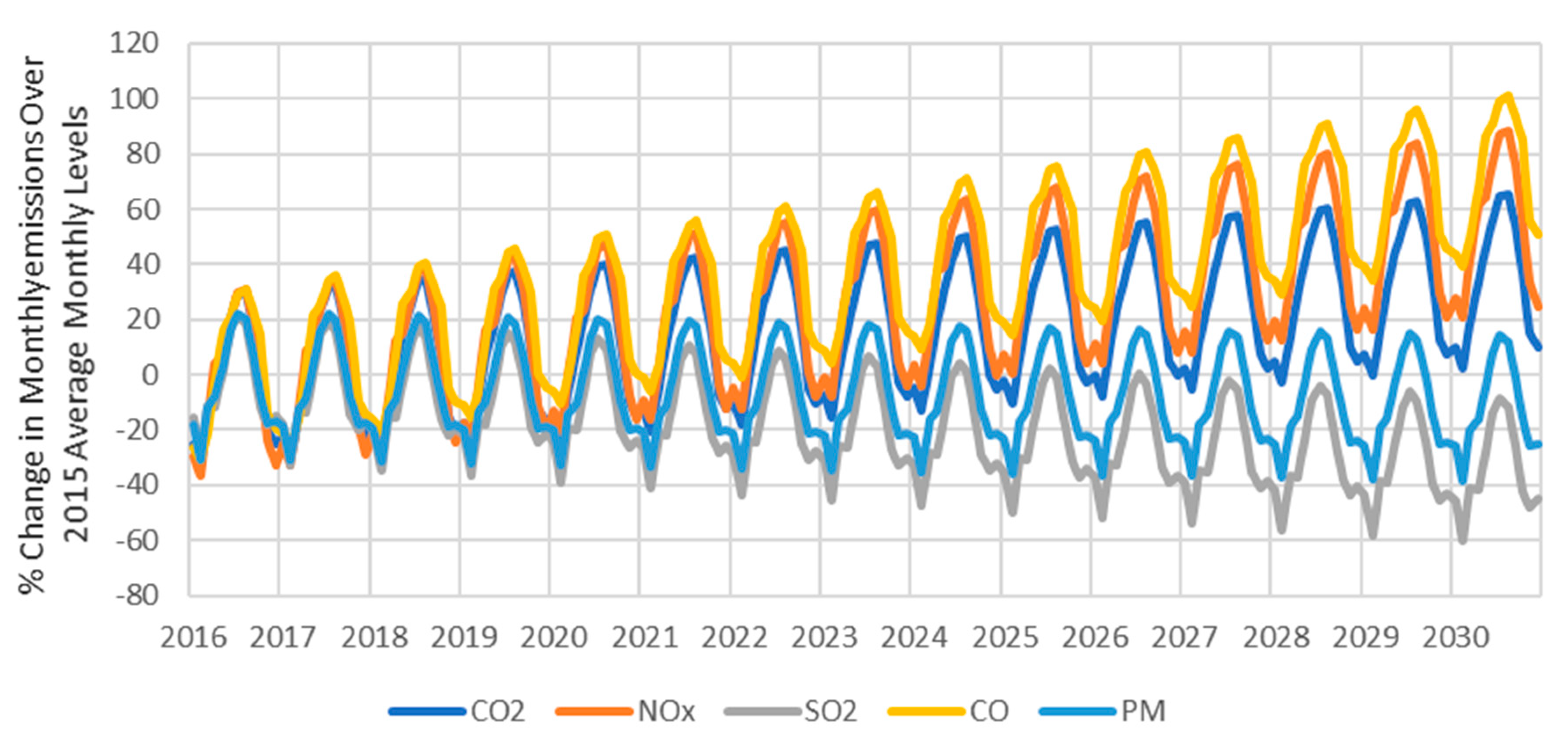
Moreover, monthly levels are higher during the summer season for all pollutants, which is a result of the increased energy demand during the hotter months of the year (see Figure 6). However, SO₂ emissions are perhaps slightly lower than 2015 levels for every projected year forward, peaking at approximately 20% during the summer season of the first projected year, which is strictly the effect of higher energy demands. However, the summer time monthly level was still only 15% lower by 2030 compared to the 2015 monthly average level. Similarly, monthly PM₁₀ emissions were effectively unchanged going forward, peaking at 15% during the summer season of 2030 compared to 22% during 2016. Every other air pollutant increased dramatically. The increase in CO and NOx emissions was driven by the expected higher penetration of natural gas and gas oil-fired technologies. The summer emission levels for 2030 were effectively double those of 2015 emission levels for CO and NOx. Not too far behind were CO₂ levels, which stood at a slightly lower 64% for the summer of 2030 compared to 2015 levels.

4. Conclusions

In this paper, unit-based emission inventories were estimated on the basis of unit-by-unit source data and calculations, the current state of which was analyzed on the basis of units grouped by combustion technologies, and future projections were assessed. Future studies can focus on developing an enhanced version of the model with up-to-date data on fuel consumption and power production infrastructure in Kuwait. The study focused on the associated temporal patterns of five major air pollutants for which power plants are a major source, namely, CO₂, NOx, SO₂, CO, and PM₁₀. In estimating future energy demand (and consequently associated emissions), a multivariate regression model that accounted for the seasonality in energy demand was developed. Consequently, this would reflect MEW’s plans for further expansion in power production infrastructure by assuming that fuel-fired technologies’ shares of production would change as per historical rates.

The annual emissions of the years 2010 to 2015 were estimated. It was observed that SO₂ as well as PM₁₀ emissions were decreasing. The other air pollutants showed a consistent increase over the years of the study. Growth rates for CO₂, NOx, SO₂, CO, and PM₁₀ stood at 19.6%, 35.7%, −13%, 41.9%, and −2.3%, respectively, by 2015 compared to 2010 levels. On a daily basis, emissions peaked during the summer season of heightened electricity consumption and stood at a minimum during the colder months. Furthermore, a seasonal hourly analysis was conducted on the basis of the respective pollutants’ highest days of emissions for every season. The diurnal patterns of all the pollutants were similar (albeit differing in magnitude from one season to the other), peaked at approximately noon, and were a minimum at night.

The analysis results revealed significant differences among the cases because the days with the highest emission rates did not necessarily correspond to the days with the highest electrical loads or fuel consumptions given that emission rates largely depend on the fuel mix used at each power station rather than the actual mechanics of electricity production. This was supported by the 53% and 55% differences in SO₂ emission rates for the second and third cases over the first case, respectively.

Future predictions of energy demand show that the demand is expected to grow at an annualized rate of 2.8% going forward, making the total growth rate of energy demand 41.6% by 2030 compared to 2015. This would require an estimated 21.8 GW in power plant-installed capacity to meet the future demand by 2030 (a 34% increase in capacity compared to 2015 levels). The annual shares of energy production for NG, GO, CO, HFO, and renewables as of 2015 stood at 51.2%, 10.7%, 3.1%, 35%, and 0%, respectively. This is expected to consequently change per MEW’s plans to 55.8%, 12.8%, 0%, 23.3%, and 8.1% by 2030, resulting in no reductions in emissions associated with energy production and, at best, could keep them at the same levels of 2015. Annual emission levels were predicted to grow by 34.3%, 54.8%, −34.3%, 71.8%, and −11% for CO₂, NOx, SO₂, CO and PM₁₀, respectively, by 2030 compared to 2015 levels.

The results show that even the ambitious 15% penetration of renewables and the increased penetration of natural gas and gas oil consumption by 2030 would not have that great of an impact on reducing emissions, and a more ambitious target of emission reductions needs to be set. Because increasing the resultant emissions of NOx, CO, and CO₂ will reduce the emissions of SO₂ and PM₁₀, a problem is essentially solved by replacing it with another. Renewables should have a higher share of the energy production infrastructure moving forward, in addition to perhaps mitigating much of the emitted pollutants at points of release by employing control equipment at power plants.