Valuing Biodiversity in Life Cycle Impact Assessment

Abstract

In this article, the authors propose an impact assessment method for life cycle assessment (LCA) that adheres to established LCA principles for land use-related impact assessment, bridges current research gaps and addresses the requirements of different stakeholders for a methodological framework. The conservation of biodiversity is a priority for humanity, as expressed in the framework of the Sustainable Development Goals (SDGs). Addressing biodiversity across value chains is a key challenge for enabling sustainable production pathways. Life cycle assessment is a standardised approach to assess and compare environmental impacts of products along their value chains. The impact assessment method presented in this article allows the quantification of the impact of land-using production processes on biodiversity for several broad land use classes. It provides a calculation framework with degrees of customisation (e.g., to take into account regional conservation priorities), but also offers a default valuation of biodiversity based on naturalness. The applicability of the method is demonstrated through an example of a consumer product. The main strength of the approach is that it yields highly aggregated information on the biodiversity impacts of products, enabling biodiversity-conscious decisions about raw materials, production routes and end user products.

1. Introduction

This paper outlines a concept for including biodiversity in life cycle assessment (LCA) to enable a look at biodiversity conservation from a product (or value chain) perspective. The aim of the paper is to present a new method that allows the assessment of potential impacts of land-using production processes on biodiversity all over the world by integrating the concept of hemeroby into a mathematical framework.

Biodiversity is defined as the variety of life on Earth at any level of organisation, ranging from molecules to ecosystems across all organisms and their populations. It includes the genetic variation among populations and their complex assemblages into communities and ecosystems [1]. Biodiversity conservation is nowadays recognized as a global priority due to its essential contribution to human well-being and the functioning of ecosystems [2,3]. However, global biodiversity is under severe threat. The International Union for the Conservation of Nature (IUCN) and the European Commission [4] recently declared that “Biodiversity loss has accelerated to an unprecedented level, both in Europe and worldwide. It has been estimated that the current global extinction rate is 1000 to 10,000 times higher than the natural background extinction rate.” Similarly, the recent report of the Intergovernmental Science-Policy Platform on Biodiversity and Ecosystem Services [5] concluded that “Nature and its vital contributions to people, which together embody biodiversity and ecosystem functions and services, are deteriorating worldwide”. The drivers of this biodiversity crisis are mostly anthropogenic and include habitat change, anthropogenic climate change, invasive alien species, overexploitation of natural resources, pollution and contamination as well as indirect drivers [6]. Many of these drivers are addressed in the Sustainable Development Goals (SDGs) adopted by the United Nations in 2015 [7], particularly in SDG 14 Life below Water and SDG 15 Life on Land. However, another key SDG impacting biodiversity is SDG 12 Responsible Production and Consumption.

Considering SDG 12, there is an urgent need to address the relationship between production and consumption and biodiversity. In fact, much of the biodiversity loss in the past and present is related to production processes that in turn depend on the increasing demand for products (i.e., consumption). Land use and associated habitat degradation followed by biodiversity loss often take place far from the location of consumption because of globalisation and the increasing level of international trade [8]. To quantitatively express and explicitly discuss the relation between consumption of products and environmental impacts, life cycle assessment (LCA) can be used as a method. By means of LCA, potential environmental impacts of products (including goods and services) are assessed along their whole life cycle (from cradle to grave) [9]. While LCA does cover a broad range of environmental impacts, biodiversity loss is not commonly addressed due to lack of an appropriate methodology.

2. Materials and Methods

2.1. Established LCA Principles

The impact assessment method we propose is intended as a sub-method of the life cycle assessment method. LCA has been an established method to analyse the potential attribution of environmental impacts of value chains to products for over 30 years. Its principles and requirements are specified in ISO 14040 [10] and ISO 14044 [11]. The goal of an LCA is to highlight hotspots of potential environmental impacts in production processes, to compare the potential impacts of alternative materials and to improve the environmental performance of products. Potential impacts are assessed via a number of impact categories, e.g., climate change, acidification and land use. The following four steps are determined by the ISO. In the first step, the system under investigation and the objectives of the LCA are defined including the system boundaries and the relevant impact categories. In the second step, the product inventory is analysed, i.e., all material and energy inputs and outputs for all processes in the value chain are compiled. The third step is the impact assessment as such. The system inputs and outputs are quantified for each impact category. For example, for the impact category Global Warming, this means that the data is translated into an amount of CO₂ equivalent. The last step of an LCA is the presentation and interpretation of the results. A detailed description of LCA and its features can be found in Hauschild et al. [12].

The method introduced in this article can be categorized as an impact assessment method for the integration of biodiversity into LCA. In fact, it is an impact assessment method which aims to quantify potential environmental impacts of land use on biodiversity. The development of impact assessment methods quantifying land use impacts started in the early 1990s with Heijungs et al. [13]. They were the first to describe the impact of land use as the product of area and time, but at that point without the consideration of soil qualities. Later on, the UN Environment Life Cycle Initiative (formerly known as UNEP-SETAC Life Cycle Initiative) defined the impacts of land use as a function of quality (Q), area (A) and time (t) [14,15]. In this framework, the quality can be any indicator on which land use of a specific area has an impact over a specific period. For example, soil quality, water storage capacity or, as presented in this article, biodiversity. Two types of land use can be differentiated—land transformation and land occupation [13]. As illustrated in Figure 1, land transformation is the change from a reference situation (Q_ref) to another quality status at one specific time (t₀). Occupation means the continuation of the (typically lower) quality status over a time period (from t₀ to t_fin). The change of the quality (ΔQ) can either be temporary if it is reversible, or permanent if it is (partly or entirely) irreversible.

This approach is the basis for all impact assessment methods quantifying impacts of land use, and thus also for the method presented here.

2.2. State of the Art in Biodiversity LCIA

One consensus in LCA research is that beside climate change, pollution, unsustainable use of resources and invasive species, the main threat to biodiversity is the loss of habitat driven by the use of land for anthropogenic purposes [16]. Thus, biodiversity, including genetic, species and ecosystem diversity as defined by the Convention on Biological Diversity [1], can be one aspect that represents quality (Q) within the framework presented ahead (see Figure 1). Several life cycle impact assessment (LCIA) methods consider biodiversity as a so-called end point indicator. Nevertheless, there is no consensus on which indicators to use to represent impacts of land use on biodiversity in LCIA. In current research, two main directions can be distinguished: LCIA methods which link land use to species richness (positing: Q = species richness), and LCIA methods which link ecological conditions to impacts on biodiversity (positing: Q = function of ecological conditions). For the former approach, species richness of e.g., vascular plants is commonly used as an indicator, often amended with species richness of several animal taxa [8]. The latter approach is usually based on a set of quantifiable conditions, e.g., deadwood availability in forest ecosystems [17] or various sets of parameters relevant to each land use type [18]. Additionally, new developments also aim to assess the impacts on functional diversity (e.g., [19]). However, these are only applicable in very limited contexts to date. The LCIA method presented in this article calculates the impact on biodiversity based on the conditions that in all likelihood define the biodiversity on the patch of land under investigation.

2.3. Requirements of Various Stakeholders

The development of a new LCIA methodology needs to take into account the requirements of various stakeholders. We distinguish four groups of stakeholders:

• addressees of LCA results, i.e., decision makers that use LCA for decision support;
• everyday LCA practitioners that provide LCA as a service to the addressees;
• the scientific LCA community that develops sub-methods within the LCA framework, to be applied by the practitioners and
• conservationists from whose realm we as LCA developers adopt methods for use within the LCA methodology.

2.3.1. Requirements of LCA Addressees

Ultimately, LCA is used for decision support. Be it policy makers writing laws or negotiating subsidies for specific technologies, be it board members of corporations strategically acquiring promising start-up companies, be it mid-level managers allocating R&D personnel to the development of new products, or the humble everyday consumer picking items from shelves in grocery stores and they all make decisions of environmental relevance. They need information about the environmental implications of products and technologies, and LCA is one of the most prominent tools to provide that information.

The above list illustrates the breadth of decision types that can—and should—benefit from LCA information. It follows that a good LCIA method should be able to provide highly aggregated information for quick everyday decisions (e.g., consumer choices), as well as more nuanced results for more complex decisions (e.g., policy design, company strategies).

Some decisions are a choice between alternatives (e.g., grocery shopping), other decisions are more proactive and creative (e.g., product development). LCA results need to be tailored to the specific addressee in order to be actionable for them: A simple “product A is better than B” or a more nuanced “this product system does not realise its full potential at these three points”, depending on the context. Company executives in particular want normative reliability, i.e., the direction of an indicator should preferably be stable. What is considered favourable today should still be considered favourable tomorrow.

There is a potential environmental benefit from LCA, but it is only realised indirectly through decision makers being addressed by LCA studies. If the information that is the result of LCA calculations is not tailored to the type of decision maker and the type of decision at hand, LCA fails to deliver its environmental benefit. In consequence, while there are other demands to be fulfilled in developing a new LCIA method, the requirements of LCA addressees weigh heaviest.

2.3.2. Requirements of LCA Practitioners

The requirements of LCA practitioners primarily address input data for LCA. The modelling of the inventory is typically the most time-consuming phase of any LCA study. A reduction of the effort for data collection and processing is therefore desirable. Data should also not be so specific over time that results based on them become worthless within a short period of time. Since data are often not available at the desired level of detail, a method for impact assessment must also be able to process coarser data and yet deliver meaningful results. Finally, the data must be reliable, which means that their sources should be traceable and transparent.

A central objective of life cycle assessments is to compare products with the same function but different manufacturing routes and thus show optimisation potentials or trade-offs from an environmental point of view. Impact assessment models must therefore be developed in such a way that these differences can be mapped and lead to different results [20].

2.3.3. Requirements of the Scientific LCA Community

The Life Cycle Initiative has formulated frameworks and guidance for the scientific LCA community in various articles [15,21] and white papers [22]—see also Section 2.1. Any impact assessment method that interprets biodiversity as a property of land needs to ensure compatibility with the land use framework. While Koellner et al. [15] and Mila i Canals et al. [21] elaborate on the differentiation between land occupation and land transformation, as well as how to account for impacts that occur over time, the discussion is mostly about processing inventory data. In terms of land use in LCA, the area (A) and the duration (Δt) of a land-using process can be understood as inventory flows. In fact, they are often combined into one flow called areatime (given in square metres multiplied by years, or m²a).

The central point of contact between impact assessment methods and the land use framework is the quality dimension (Q). A new LCIA method has to deliver both a Q(t) value at any point on the time axis and a reference value (Q_ref) in order for the quality difference ΔQ(t) to emerge as a characterisation factor, to be multiplied with the areatime inventory flow (see also Figure 1).

Compliance with this requirement means that a quality value must be independent from the area affected and the duration of the effect. While it is true that more damage to biodiversity is caused by an activity on a larger area over a longer duration, area and time are independent factors in the impact calculation. They do not influence the definition of points on the Q axis. In mathematical terms, the three dimensions Q, A and t are not spatial dimensions, but form a de-facto Euclidean vector space.

That said, the provision of a Q_temp value is often easier than the provision of a Q_perm value. If the approach is limited to temporary impacts (also known as occupation impacts), then data on the temporal extent of a particular land-using activity are usually available. As a rule, agricultural and forestry activities are conducted with an indefinite time horizon, but it is possible to calculate annually averaged Q(t) values. Permanent quality differences (ΔQ_perm) are typically only available if a land-using activity is inherently limited in time (e.g., mining).

General methodological requirements for LCA (beyond specific requirements for land use) also impose a series of ISO standards: ISO 14040, [10] ISO 14044 [11] and ISO 14067 [23]. The first two standards refer explicitly to LCA, but do not contain specific references to impact aspects such as land use or biodiversity. ISO 14067 [23] refers to carbon footprinting, but is closely related to the LCA methodology. This standard incorporates a number of aspects for the calculation of land-use aspects: the question of direct or indirect land-use change, temporal aspects such as the question of delayed release or removal of carbon. For the application, however, the requirements have little reference to quality-related assessment of land areas such as biodiversity. Indirect land use and delayed processes are undoubtedly relevant for biodiversity consideration in global value chains, but both these sub-topics are inventory matters, and thus outside the scope of the method presented here. We aim to provide a framework for the calculation of a Q(t) value for any kind of terrestrial surface (i.e., impact assessment). If an inventory method provides the location and land use type of an indirectly affected patch of terrestrial surface, the method presented here can generally be used to characterise the damage incurred on that patch.

Last but not least, a concern of the scientific community is that LCA can be misused or downright corrupted by practitioners or addressees with vested interests. LCA is rooted in the natural sciences, but this also means that it tends to yield complex and contradictory results that are open to interpretation and can be strongly context-dependent. With its aura of factuality combined with the inherent complexity, LCA lends itself to manipulative applications [24]. A new sub-method for LCA should be structured in a way that minimizes the danger of improper use.

2.3.4. Requirements of Conservationists

Biodiversity is a distinctly multidimensional property. In consequence, ecologists and conservationist find it difficult to quantify, partly because of the multitude of indices proposed for this purpose [25]. Unfortunately, there is no common consensus about which indices are more appropriate and informative although they are the key for environmental monitoring and conservation. Furthermore, the metrics used to measure biodiversity have to fulfil certain requirements to be compatible with use in LCA. In their recent review, Curran et al. [26] performed a meta-analysis and ranked studies based on a number of parameters. From a conservationist point of view, biodiversity representation both on a local and regional scale and the reference state play a major role. As detailed in Curran et al. [26], a number of attributes are required to reflect the multidimensional nature of biodiversity, e.g., function, structure, composition. Moreover, several taxonomic groups and spatial scales should ideally be considered. Local and regional components should be presented separately and the regional importance of biodiversity should be qualified by rarity, endemism, irreplaceability and vulnerability. Finally, the historic potential natural vegetation may not be the most appropriate reference state.

The complexity of biodiversity and ecosystems should not be underestimated, consequently many conservationists may be more comfortable with a bottom-up method for biodiversity quantification in contrast to a top-down approach. If a top-down approach lacking in empirical data is adopted, ecologists and conservationists will require any proposed methodology to reflect biodiversity in a meaningful way. For instance, the choice of index can profoundly influence the outcome [25]. In summary, any LCA indicator quantifying biodiversity should conform to conservation efforts, i.e., good or best practice management should be reflected in a favourable LCA indicator score, while intrusive interventions should be punished.

2.4. Research Gaps

Even though the inclusion of biodiversity into LCA practices is a research question for which a variety of approaches have been suggested for more than 20 years, some essential gaps and challenges exist [16]. Based on Winter et al. [16] and in order to address as many gaps as possible, more than 25 published impact assessment methods for evaluating impacts of land use on biodiversity were screened for different characteristics like the impact category they cover, their resolution and geographical coverage etc. The literature analysis was a preliminary step for the method development presented here. In summary, most of the methods presently available are designed for integration into LCA. Nevertheless, the application of these is very limited. One of the reasons could be that the available impact assessment methods differ greatly. For example, the number of considered land use classes vary from six [8] up to 44 [27]. Most allow differentiation between extensive and intensive land use. Additionally, methods distinguish between forestry, pasture and crops [18,28,29]. Nevertheless, the level of differentiation markedly varies. A stronger consensus has been found for the types of land use change under consideration. All methods assess the impacts of direct land occupation changes, meaning land transformation is not assessed at all. Also the differentiation of sites is very similar between the investigated impact assessment methods. Usually the different biomes or ecoregions are considered [16]. However, most of the methods are not globally applicable because the available data cover only specific regions [16]. The potential natural vegetation is most frequently suggested as the reference state, although other references like the current state of the vegetation are also taken into account in some methods. Finally, two approaches of considering the impacts of land use on biodiversity or ecosystems in LCA are available within the examined impact assessment methods. First, considering the impacts on species or second, on conditions favourable for biodiversity. The study at hand proposes a method addressing the latter.

3. Proposal for a Biodiversity Impact Assessment Method

The authors propose a biodiversity impact assessment method that combines the fuzzy framework from Lindner [20] and Lindner et al. [30,31,32] with the hemeroby approach by Fehrenbach et al. [33] in a framework previously proposed by Maier et al. [18]. Fehrenbach et al. [33] equate naturalness with a high biodiversity value, but provide only a rough calculation structure. Lindner [20] and Lindner et al. [30,31,32] posit a relatively fine-grained calculation structure for biodiversity value, but stop short of making a strong case for what that value should be. Maier et al. [18] use a regional weighting factor, fixed intervals per land use type, and a set of management parameters per land use type. Different combinations of two of these elements have been proposed before [20,29], but all three are combined into one framework by Maier et al. The method presented here was developed to address the above mentioned requirements for different stakeholders and to fill research gaps in this field. This Section outlines the mathematical structure of the method. An example calculation is provided in Section 4.

Biological diversity, as defined by the Convention on Biological Diversity (CBD) [1] describes variability at different levels, apart from species diversity, the variability within species (genetically), as well as ecosystems and functions. The approach described here does not explicitly focus on a specific level of biodiversity. By connecting to criteria for naturalness, however, strong reference is made to the ecosystem level. There is evidence that decline in biodiversity correlates with a decreasing number of habitat niches. For instance, the naturalness of an agricultural ecosystem correlates with the diversity of structures [34,35,36]. Winter [37] identified forest naturalness as a component of biodiversity monitoring. More naturalness—less hemeroby—is therefore one of the most important prerequisites for the conservation of global biodiversity. However, please note that the biodiversity value calculation framework presented in this Section is not based on empirical data, but rather our suggestion. Given the numerous and diverging demands from various stakeholders (see Section 2.3), we propose the framework at hand. It is meant to capture the complexity of biodiversity and yet provide a singular meaningful indicator that points in the right direction. In this context, it should be pointed out that the response variable (i.e., the calculation result, the “biodiversity number”) is not a physical measurement but a philosophical quantity with a strong normative component. Readers familiar with multi-criteria decision analysis (MCDA) will find that the method presented bears some similarity to some MCDA methods (most notably, methods based on fuzzy modelling; see e.g., [38]). Both the characteristics of the response variable and the structure are discussed in Section 5.

3.1. Overall Structure

The method we propose produces a quality indicator for a given patch of land, that is to say a Q value for use in the Q, A, t diagram of the land use framework referenced in Section 2.1. The input data from which the Q value is calculated are properties of the land; mostly management parameters. The calculation follows a sequence of steps that is structurally the same regardless of which kind of land use is assessed:

• Each parameter input x is transformed into a biodiversity value contribution y by means of a biodiversity contribution function y(x).
• One or more biodiversity value contributions (e.g., y_A and y_B) are aggregated into a criterion z by means of an aggregation function; e.g., z_AB (y_A, y_B).
• Several criteria (e.g., z_AB and z_CD) are aggregated into the land use-specific biodiversity value BV_LU by means of a linear function; e.g., BV_LU (z_AB, z_CD).
• The land use specific biodiversity value BV_LU is transformed into the local biodiversity value BV_loc by fitting the interval of possible BV_LU values into the interval between the minimum and maximum local biodiversity value.
• The local biodiversity value BV_loc is transformed into the global biodiversity value BV_glo by multiplication with the ecoregion factor EF. This BV_glo is the end result, i.e., the Q value for further use in the land use framework.

While the sequence of the steps is fixed, some steps include customised transformations. The biodiversity contribution functions y_ijk (x_ijk) for step 1 are specific to the parameter i, the land use class j and the biome k. The nonlinear aggregation functions z_hjk (y_ijk) for step 2 are specific to the criterion h, the land use class j and the biome k. The linear aggregation functions for step 3 are specific to the land use class j and the biome k.

This means that the method allows differentiation between sites (biomes and ecoregions) and between practices (land use classes and management parameters). For differentiation between land use classes, each class is assigned a minimum and a maximum (land use-specific) biodiversity value, creating an interval for the BV_LU (see Figure 2). Within this interval, the biodiversity contribution functions of each parameter are used to navigate between the minimum and the maximum value. If all parameters are at the best level for high value biodiversity, then the BV_LU reaches its maximum.

For the differentiation between biomes, the biodiversity contribution functions y(x) are modified. In one biome, the valuable biodiversity might be more susceptible to nutrient overload than in another. In both biomes, the parameter addressing nutrient overload would be part of the land use-specific biodiversity value, but the contribution to the biodiversity value would deteriorate more quickly (at lower nutrient input) in one biome than in the other.

The differentiation between ecoregions is implemented in step 5. Essentially, the ecoregion factor is a weighting factor that makes the biome-specific and land use-specific biodiversity values globally comparable. Assume that one ecoregion has a factor twice as high as another ecoregion, then each m² with a given BV_LU counts twice as much globally as each m² with the same BV_LU in the other ecoregion. This also means that land-using processes that deteriorate the biodiversity value of the land on which they are implemented are twice as destructive in the former ecoregion than in the latter. In other words, the ecoregion factor addresses the question: “How much worse is it to destroy half the biodiversity on a km² in the Peruvian Yunga versus half the biodiversity on another km² in the Siberian Tundra”?

It is possible to assume a “typical” BV_LU for the various land use classes. For instance, a product made from e.g., cotton is to be evaluated, but no data on the production of the raw material are available other than “it is cotton from Brazil”. In this case, the LCA practitioner would use the typical BV_LU for “agriculture, intensive, Brazil” rather than collect all parameter input data from all suppliers of the cotton trader (unless the project is big enough and calls for such breadth and depth). If, however, the manufacturer of the cotton product has a specific supplier and together they want to improve the biodiversity impact of their product, all parameter input data can be collected from this one supplier.

Typical hemeroby levels for a variety of land use types are provided, e.g., by Fehrenbach et al. [30], referring to Giegrich and Sturm [39]. Brentrup et al. [40] also give examples of hemeroby classes assigned to land use types (using 10 hemeroby levels, but the principle is the same).

The method dovetails with the land use framework mentioned in Section 2.1, i.e., it provides a biodiversity value and a reference state. Both are required to calculate the quality difference. In conjunction with the areatime demand of the land-using process in question, the ΔQ is used as a characterisation factor for land use LCIA. From there, all LCA calculations follow as per the state of the art.

The unit of the biodiversity quality is the biodiversity value increment (BVI). It is a purely artificial unit for comparisons.

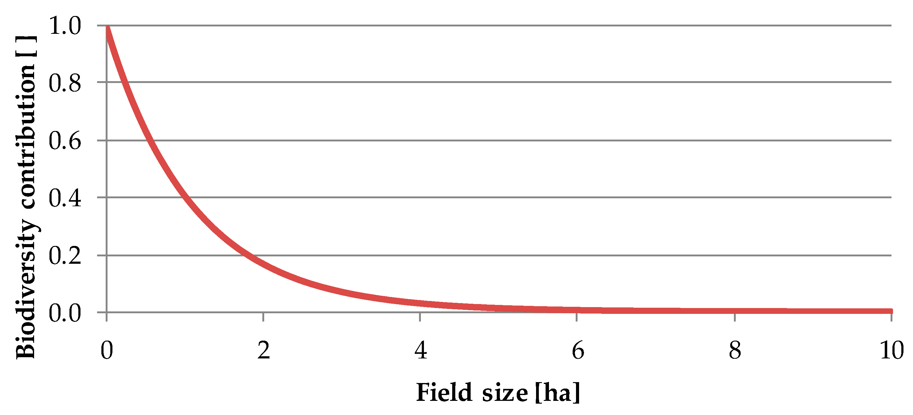
3.2. Biodiversity Parameters and Their Contributions to the Biodiversity Value

While the mathematical framework outlined in Section 3.1 does not prescribe how to measure biodiversity, we use naturalness as a proxy for valuable biodiversity. The working assumption is that the more natural a patch of land is, the higher the value of the biodiversity it hosts. Naturalness is quantitatively expressed by hemeroby (deviation from nature), so a high hemeroby level implies low naturalness and low biodiversity value. In particular, we integrate the hemeroby concept as previously adopted for LCIA by Fehrenbach et al. [33]. Note that man-made ecosystems (such as agrarian landscapes and even mining sites) can have degrees of naturalness even though they would not exist without continuous intervention.

The concept of Fehrenbach et al. [33] defines separate catalogues of criteria for the evaluation of hemeroby for each of the land use categories forest, agriculture and urban areas. The criteria for forest land refer to the ground work of Westphal and Sturm [41], who derived three criteria and 20 parameters (metrics) for assessing the hemeroby of forest systems (in particular for the biome “temperate broadleaf forests”. The criteria distinguish between naturalness of the soil, naturalness of the forest vegetation, and naturalness of the development conditions. A number of metrics is assigned to each criterion, which are assessed in an ordinal form with five tiers.

The tiers are defined by descriptive texts, often addressing more than one parameter. A parameter is the smallest and most detailed measurable unit described in a metric. Take the criterion naturalness of the soil, for example: The metric “intensity of mechanical earth working” of the land use class forestry is divided in the parameters “shallow mechanical earth working” and “deep mechanical earth working”. To combine this method with the one from Lindner [20,30], a function has to be modelled for each parameter. Because of the ordinal system provided in the literature, the biodiversity contribution function of a hemeroby parameter contains steps. For example, the parameter “field size” in the land use class “arable” is associated with a hemeroby level from 1 to 5 on the overall hemeroby scale from 1 to 7 (see Figure 3; high hemeroby means more impact). The complete list of metrics and parameters is included in Supplementary Materials.

In the original hemeroby literature (for example by Jalas [42] and Sukopp [43]), the hemeroby scale is an ordinal scale, but it is transformed into a cardinal scale here. Fehrenbach et al. [30] used a linear transformation (which we apply here as well), but also discussed an exponential transformation. Brentrup et al. [40] also opted for a linear transformation. Ultimately, there is no correct way, because the transformation is, in a strict sense, impossible. Bearing in mind the incompatibility of the ordinal and cardinal scales, transformation is carried out here nevertheless for the sake of practicality. Other proponents of hemeroby in LCIA have also argued for the ordinal-to-cardinal conversion on grounds of practicality [30,40].

The hemeroby function for a parameter is essentially its biodiversity contribution function, but it requires transformation to fit into the framework of the overall method. Once the hemeroby function is established, it is inverted, so that the hemeroby axis descends. We make the simplifying assumption that a lower hemeroby level corresponds to a higher biodiversity value. The descending hemeroby axis is thus relabelled into the ascending biodiversity contribution axis (see Figure 4; low biodiversity contribution means more impact). The axis is normalised to the [0, 1] interval, so that the highest hemeroby level corresponds to zero biodiversity value and the lowest hemeroby value corresponds to a biodiversity contribution of 1.

In the specific example of field size, thresholds between the hemeroby levels are derived from an Austrian directive [44]. The biodiversity value descending to zero at 2.25 ha (Figure 4) does not imply that a field larger than that has no biodiversity value. The biodiversity contribution is aggregated with the biodiversity contributions of other parameters (see below). The field may well have a biodiversity value greater than zero, but that value would be assigned based on contributions from other parameters.

The stepwise function is replaced by a smooth, differentiable function—the biodiversity contribution function y(x) for the parameter in question (see Figure 5; low biodiversity contribution means more impact). Every biodiversity contribution function is developed from the same basic equation that describes y as a function of x with six constants alpha α, sigma σ, beta β, gamma γ, delta δ and epsilon ε (see Equation (1)). The constants allow shaping the curve into any desired shape (see [20,30]). They are considered malleable when defining the y(x) function, but remain constant once it is defined.

$$\mathrm{y}=\mathsf{\gamma }+\mathsf{\epsilon }\ast \exp \left[-\frac{\left|{\left({\mathrm{x}}^{\mathsf{\delta }}-\mathsf{\beta }\right)}^{\mathsf{\alpha }}\right|}{2{\mathsf{\sigma }}^{\mathsf{\alpha }}}\right]$$

(1)

We used a least-squares fit, but any fitting method will do. Some boundary conditions apply: The smooth function needs to hit the exact values of the stepwise function at x = 0 and x = 1, and the biodiversity contribution y needs to stay in the [0, 1] interval.

3.3. Biodiversity Criteria

The criteria values mentioned in Section 3.1 can be understood as aggregated biodiversity contributions from multiple parameters. For example, in the “agrarian” land use class, one criterion is soil treatment (A.3), which comprises two parameters: how much soil is moved each year (A.3.1), and the length of time over which the soil is left uncovered (A.3.2). Each parameter has its biodiversity contribution function y(x). Both biodiversity contributions are aggregated into the criterion z_A.3(y_A.3.1, y_A.3.2).

Two essential aggregation operations are available for the development of a criterion function z(y); i.e., the AND and the OR operations. The AND operation represents a situation in which multiple parameters need to yield a high biodiversity contribution in order for the criterion value to be overall high. If either of the parameters yields a low biodiversity contribution, the criterion value is low. The OR operation represents the opposite situation—As long as either one of the parameters yields a high biodiversity contribution, the criterion value is high. Their respective equations for any number s of criteria are Equation (2) for AND, and Equation (3) for OR.

$${\mathrm{y}}_{\mathrm{A}\dots \mathrm{s}}\left({\mathrm{x}}_{\mathrm{A}},\dots ,{\mathrm{x}}_{\mathrm{s}}\right)=1-\sqrt[\mathrm{p}]{\frac{1}{\mathrm{s}}{\displaystyle \sum }_{\mathrm{i}=1}^{\mathrm{s}}{\left(1-{\mathrm{y}}_{\mathrm{i}}\left(\mathrm{x}\right)\right)}^{\mathrm{p}}}$$

(2)

$${\mathrm{y}}_{\mathrm{A}\dots \mathrm{s}}\left({\mathrm{x}}_{\mathrm{A}},\dots ,{\mathrm{x}}_{\mathrm{s}}\right)=\sqrt[\mathrm{p}]{\frac{1}{\mathrm{s}}{\displaystyle \sum }_{\mathrm{i}=1}^{\mathrm{s}}{\left({\mathrm{y}}_{\mathrm{i}}\left(\mathrm{x}\right)\right)}^{\mathrm{p}}}$$

(3)

Both equations can be customised by altering the exponent p. The higher the exponent, the stricter the aggregation function becomes. While the default exponent is 2, it may be 5 or higher for a rather strict AND function. Exponent = 2 means that if one biodiversity contribution is zero, a limited criterion value can still be achieved if the other parameters yield a high biodiversity contribution (visualised for the AND aggregation in Figure 6). Exponent = 5 or higher makes this kind of compensation all but impossible.

The OR function shows the opposite characteristic. With the exponent at the default 2, the criterion value reaches its maximum only when all parameters yield a high biodiversity contribution, and it is medium–high if all but one parameter yield a low biodiversity contribution. With exponent = 5 or higher, the low biodiversity contributions from some parameters are all but irrelevant as long as one parameter in the same criterion yields a high contribution.

A special case is the AND/OR criterion with exponent = 1. In this case, the biodiversity contributions from the parameters are aggregated in a linear fashion. Mathematically, the criterion value then is the arithmetic mean of the biodiversity contributions.

The criteria values are aggregated into the land use-specific biodiversity value BV_LU of a plot. This step is a simple weighted summation. Each criterion is multiplied by a factor and the sum of the weighted criteria values is the BV_LU. The interval for BV_LU is also [0, 1], so the sum of the weighting factors needs to be 1. Unless there is an indication that the criteria are not equally relevant for the biodiversity value, the default weight is 1/n (with n being the number of criteria for the land use class).

3.4. Global Weighting

The biodiversity value calculated from parameters and criteria distinguishes biomes, i.e., biodiversity contribution functions and criteria functions may vary between biomes. This differentiation is further refined by applying a global weighting factor. It allows for finer biogeographical differentiation than biomes and is at the same time not too labour-intensive to use in practice because there is no need for new impact functions on the finer geographical level.

Our global weighting factor distinguishes ecoregions worldwide (as defined by Olson et al. [45]) and is called ecoregion factor (EF). It aims to include the three dimensions of biodiversity by integrating different indicators which reflect genetic diversity, species diversity and ecological diversity. The approach is inspired by the location factor of Brethauer [46]. Essentially, an ecoregion with a high EF is more valuable in the global comparison than an ecoregion with a lower EF, and damage incurred by a plot in the high-EF ecoregion is amplified.

The EF comprises four indicators on the ecoregion level: the area share of grassland and forest (SGF), the area share of wetlands (SW), the Global Extinction Probabilities (GEP) and the Share of Roadless Areas (SRA). The indicators SGF and SW aim to represent main habitats. They are not differentiated on a finer geographical level, because they aim to display these habitats all over the world. The data for the SGF was gathered by Winter et al. [47]. The SW was calculated by the area of wetland (downloaded from The Ramsar Convention Secretariat [48]) per ecoregion. The GEP is taken from Kuipers et al. [49] and the SRA from Ibisch et al. [50]. All indicators are normalised to the [0, 1] interval, i.e., the lowest value for each indicator across all ecoregions is 0 and the highest value is 1. The EF is calculated according to Equation (4) with the considered indicators. This is effectively a variation of Equation (2) with four inputs, but is independent of the criteria mentioned in Section 3.3.

$$\begin{array}{c}\mathrm{EF}=1-\sqrt[2]{\frac{1}{4}\left({\left(1-\mathrm{SGF}\right)}^2+{\left(1-\mathrm{SW}\right)}^2+{\left(1-\mathrm{GEP}\right)}^2+{\left(1-\mathrm{SRA}\right)}^2\right)}\\ \mathrm{for}\mathrm{SGF},\mathrm{SW},\mathrm{GEP},\mathrm{SRA}\in \left[0,1\right]\end{array}$$

(4)

The data for all components of the EF are available for only 744 ecoregions. Thus, for less than a hundred ecoregions no EF could be calculated. The values of the EF reach from 0.035 to 0.517, so the maximum factor between the lowest and the highest EF is 15. The majority of ecoregions have an EF between 0.1 and 0.4 (see Figure 7), so in most cases the EF difference between two ecoregions is not expected to exceed a factor of four. The full list of EFs can be found in the Supplementary Materials.

4. Example

To illustrate the application of the method, we have chosen as an example a common consumer product that combines various components of land use—a classic pizza. In order to keep the example simple and illustrative, the recipe and the production process has strongly been reduced in complexity (see Figure 8). The exemplary pizza consists of a wheat dough with a base layer of strained tomatoes. We consider only two toppings, namely pork salami and grated dairy cheese. The pizza is baked in a traditional wood-fired oven fed with beech logs.

Table 1. Basic data for the exemplary product system “pizza”, with raw materials sourced from the ecoregions ^(a) Western European broadleaf forests, ^(b) Cerrado and ^(c) South-eastern Iberian shrubs and woodlands.

Ingredient	Quantity per FU	Land Use Class	Ecoregion	Land Use per Ingredient	Land Use per FU
				[m2a/kg]	[m2a/FU]
wheat flour	200 g/FU	agricultural land, typical intensive cultivation	PA0445 (a)	1.5	0.3
cheese	200 g/FU	agricultural land, monoculture soybean	NT0704 (b)	4.5	0.9
salami	100 g/FU	agricultural land, monoculture soybean	NT0704 (b)	8.0	0.8
tomatoes	100 g/FU	greenhouse plantation, highly intensified	PA1219 (c)	0.05	0.005
firewood	0.002 m3/FU	forest, beech	PA0445 (a)	1000	2.0

shows the simplified pizza recipe, the land use class per ingredient, the ecoregions from which the ingredients are sourced, the land use for each ingredient (as areatime demand), and the land use per functional unit (FU, in this case one entire pizza). We have strongly simplified the feed composition for the raising of pigs (for the salami) and cattle (for the cheese) by assuming that both are raised exclusively on soy meal. Furthermore, we assume the Cerrado region in Brazil as the only origin of the soy fodder. The factors for land use (areatime per mass of ingredient) are approximations referring to recent work of Keller et al. [51].

Table 2. Calculation of the specific biodiversity value BV_arable for wheat in the “pizza” example with parameters based on Fehrenbach et al., (2015).

	Criterion/Parameter		Parameter Value	Criterion Value	Criterion Weight	Weighted Contribution [BVI]
A.1	Diversity of weeds			0.530	0.2	0.106
	A.1.1	Number of weed species	0.241
	A.1.2	Existence of rarer species	0.710
A.2	Diversity of structures			0.300	0.2	0.060
	A.2.1	Elements of structure in the area	0.424
	A.2.2	Size of cuts	0.000
A.3	Soil conservation			0.257	0.2	0.051
	A.3.1	Intensity of soil movement	0.184
	A.3.2	Ground cover	0.006
	A.3.3	Crop rotation	0.931
A.4	Fertilisation			0.068	0.2	0.014
	A.4.1	Share of farm manure	1.000
	A.4.2	Ratio manure vs. slurry	1.000
	A.4.3	Share of synthetic fertiliser	0.000
	A.4.4	Share of slurry and synthetic fertiliser beyond growth period	1.000
	A.4.5	Intensity of fertilisation	0.136
A.5	Pest control			0.708	0.2	0.142
	A.5.1	Input of pesticides	0.108
	A.5.2	Share of mechanical/biological pest control	0.995
BVarable						0.373
BVlocal						0.353

shows the calculation of the specific biodiversity value BV_LU for wheat (BV_arable for land use class “arable”). The calculation for the other ingredients is included in the Supplementary Materials. BV_arable is the sum of the weighted biodiversity contributions, in this case 0.373 (see bottom of Table 2). The “arable” class ranges from hemeroby 3 to 6. Transformed into the BV_local scale, this range corresponds to the interval from 0.167 (hemeroby 6) to 0.667 (hemeroby 3). BV_arable = 0.373 means that the BV_local level is at 37.3% of the interval for the “arable” class, i.e., at BV_local = 0.353 (see bottom of Table 2).

Table 3. Example “pizza”: aggregation of the specific biodiversity value (BV_LU) of the ingredients to the complete product and considering the ecoregion factor (EF).

Ingredient	BVlocal	EF	BVglobal = Q	ΔQ	Land Use per FU	Impact per FU = Land Use * ΔQ
	[BVI]	[]	[BVI]	[BVI]	[m2a/FU]	[BVI m2a]
wheat	0.373	0.127	0.045	0.081	0.3	0.025
soy/cheese	0.329	0.427	0.141	0.285	0.9	0.257
soy/salami	0.329	0.427	0.141	0.285	0.8	0.228
tomatoes	0.000	0.110	0.000	0.110	0.005	0.001
firewood	0.821	0.127	0.112	0.015	2.0	0.030
total						0.540

shows the aggregation of the single ingredients and the resulting specific biodiversity value BV_local for the exemplary pizza. Land use-specific Q values were calculated for all but one ingredient: we assume that the tomatoes are grown in a fairly artificial greenhouse environment, so this land use is assigned the highest hemeroby value (lowest Q value) without further consideration. This can be understood as an example for a “typical” Q value (see Figure 2) mixed with more specific values in the same product system. One interesting find is that the wood is quite area-intensive to grow (because forestry is slower at producing biomass than agriculture), and the area footprint of the wood is quite high (2.0 m²a/FU). However, the biodiversity impact of the forestry process (ΔQ) is rather low (because forestry is much less intrusive than agriculture), and so is the impact per functional unit. Another relevant point is that the ecoregion factor of NT0704 is 3.36 times higher than the factor of PA0445—in other words, that each square metre in the Brazilian Cerrado is considered much more valuable than a similar square metre in Western Europe. This difference in EF applies to the impact as well. The BV_local of the soy cultivation process is only 12% lower than the BV_local of the wheat cultivation process (0.329 vs. 0.373), but the BV_global values differ by a factor of 3.1 (0.045 vs. 0.141) due to the difference in EF.

The example shows the very different proportions of the individual ingredients in the overall result for a dish such as pizza. In this case, the animal ingredients cheese and salami make, by far, the largest contribution to the product’s biodiversity impact (see Figure 9), accounting for about 42% and 48%, respectively. Firewood and wheat play a minor role (both around 5%). Tomatoes contribute even less, although their production area is regarded as an industrial area. For our hypothetical restaurant owner, this would mean that the starting point for improving the biodiversity profile of his pizza are the cheese and the salami. He might look for another supplier that sources fodder from a less sensitive region, or go vegetarian or vegan altogether.

The results can be further disaggregated at the ingredient level. Figure 10 shows the BV_arable for the wheat provision process (see Table 2), broken down into biodiversity contributions from the five criteria. Each criterion could potentially yield a maximum biodiversity contribution (equal to its weighting factor in Table 2), but given the parameters (also Table 2), only a fraction of the potential is actually realised. For our hypothetical wheat farmer, this information would mean that he is missing out on achievable biodiversity value mostly due to fertiliser use. He might switch from synthetic fertiliser to manure and maybe reduce the total amount to some degree.

5. Discussion

5.1. Strengths of the Method

One of the prominent strengths of the proposed method is that it produces highly aggregated information as a result, yet the result can be disaggregated to the criterion level if needed. One potential question that can be answered with this method is: “Should I have the pizza with meat or the vegetarian option if I want to cause less damage to biodiversity?” A typical question for a (conscious) consumer. The (equally conscious) restaurant owner might ask: “Should I use the salami from pork raised on intensively farmed soy or the other salami from pork raised on another diet?” Lastly, the conscious soy farmer might ask: “I can accept to lose some yield for the sake of conservation, but is it better for biodiversity to cut pesticides or fertiliser?” All these actions influence the biodiversity impact of the pizza, and they all can be answered with the same consistent method. This is also possible with the approach of Maier et al. [18] even though the specific definitions of the methodological elements differ.

However, the consistency might feel somewhat forced here. Very different kinds of land use in very different biomes are not as such comparable, they are made comparable by the design of the method. Some authors (not all) believe that this is actually another strength of the method. It places the focus on the value that human societies ascribe to biodiversity rather than biodiversity as the subject of empirical study central to natural sciences. Biodiversity means more than just species richness (although it remains the most common understanding and most readily quantifiable metric of biodiversity). It includes genetic components and ecosystem components [1]. It caters to a number of societal goals [7,52]. Weighing the various components of biodiversity against each other is a normative act that is often overlooked when decision makers (addressees of LCA studies) ask for simple results à la: “Which option is objectively the better one from a biodiversity perspective?” Even if we saw purely instrumental values in biodiversity, we would need to aggregate these multiple instrumental values into a singular biodiversity value, which again would constitute a normative act. While the societal discussion about how to aggregate the many components of biodiversity and values connected to it has barely begun, the proposed method offers a starting point and allows for modifications once the discussion advances. The mathematical framework resembles a MCDA method for exactly this purpose—to allow the quantified expression of preferences. It is effectively a distance-to-target MCDA framework where the default target is naturalness, with the option to define the target more specifically where possible.

For the time being, the value of biodiversity is captured through the proxy of naturalness, or inverse-hemeroby. The hemeroby concept is relatively well grounded in literature and older than LCA [42,43] (though not undisputed). In lieu of a more elaborate valuing of the various components of biodiversity, our choice of naturalness as a proxy is a judgement call. Freidberg [24] cites an LCA practitioner who explains that for the sake of practicality, consultants who use LCA are sometimes forced to make judgement calls. It is our position that with our choice of the hemeroby concept, the unavoidable judgement call was made on the development level rather than on the practice level. Given the complexity of biodiversity as a safeguard subject, this seemed like the favourable option. Leaving this unavoidable judgement call to LCA practitioners means postponing a decision that will ultimately have to be made. Yet in all likelihood, LCA practitioners will decide with less time and a less complete understanding of impact assessment models. Moreover, they may even experience pressure by LCA addressees to tweak a study into yielding favourable results in some cases.

Another strength of the method is the actionability of the results. One of the classic LCA questions is where to focus efforts for the environmental improvement of a complex product system. Coming back to the pizza example, it is easy to identify the process that produces the highest share of the total biodiversity impact. Furthermore, each criterion across all land-using processes has a known maximum value, so it is easy to compare all criteria within the entire product system to learn how much biodiversity potential is left unrealised, i.e., where most could be gained through improvement. Going even deeper, the biodiversity contribution functions of all parameters are fully differentiable. This means it is possible to calculate the sensitivity of the entire product system to marginal changes in single parameters in individual land-using processes.

Modularity is another strength: various elements of the method can be altered without invalidating other elements – a property shared with earlier, similarly modular approaches [18,20,29]. For example, the biodiversity contribution function for parameter A.3.1 within criterion A.3 within land use class A (“arable”) in biome “Temperate broadleaf and mixed forests” can be altered with no effect even on the biodiversity contribution function of the next parameter A.3.2 in the same criterion. Biodiversity contribution functions of parameters, criterion value functions, biodiversity value functions and ecoregion factors can all be updated independently if new knowledge arises or if societal values and priorities shift. In some other methods, updating one data point necessitates recalculation of many or all other elements. For the target of the distance-to-target MCDA framework, this means that even the preferred target may be updated in one region, if the discussion is advanced far enough, without having to wait for other regions.

5.2. Weaknesses of the Method

The method presented here was specifically designed for integration into LCA. Thus, it caters to the requirements of LCA input data, which are often scarce or unavailable. All current methods are equally limited by this lack of data. However, there is an undisputable drawback in the fact that although our method proposes to quantify biodiversity, it does not actually measure biodiversity due to its top-down approach. Biodiversity is inferred by use of a number of indicators, so a considerable level of generalisation is to be expected. In other words, the proposed method may appear as a blunt instrument.

However, even the most advanced characterisation factors available to date distinguish only between five land use classes and three management levels [53]. Quite obviously, quantifying biodiversity in all its different aspects and underlying complexities is beyond one simple index or indicator; a fact that has been stated many times (e.g., [25,26]).

In this special issue, Gabel et al. [54] performed a comparative empirical test of four different methods for on-farm biodiversity assessment and concluded that no single method emerged as a clear favourite. They also correctly pointed out that a considerable level of training and expertise was required for application of some of the methods, a general challenge associated with any method or indicator based on quantifying biodiversity as species richness or abundance.

Our proposed method is designed to integrate all the different perspectives and their respective indicators into one consistent calculation framework. The weakness associated with this claim is two-fold: firstly, the method as defined here might overstretch its reasonable applicability space and secondly, the method is, from a natural science perspective, empirically untestable.

From a conservation perspective, all elements of biodiversity are individually valuable. Valuing biodiversity (as is our claim) should not mean discounting some elements of biodiversity against others. For example, the loss of a species-poor ecosystem cannot be compensated by the extension and long-term protection of a species-rich ecosystem, because the species lost are not the same as those saved. Even if they were, hypothetically, one ecosystem would still be lost, and ecosystems are also declared valuable according to the CBD [1]. Our method essentially introduces a currency for biodiversity (the BVI) and thus, by definition, makes all elements of biodiversity interchangeable. Other methods are more specific, e.g., in Environmental Impact Assessment (EIA), compensation measures for destructive land development may be prescribed. These are often (not always) carried out in relatively close proximity and thus involve at least similar ecosystems. With our method, it is theoretically possible that two product systems that impact entirely different ecosystems are assigned the same overall biodiversity impact. LCA has a much more global focus than EIA, and the generalisation may thus be unavoidable, but it is worth pondering whether this level of generalisation is even useful from a conservation perspective.

The untestability criticism is arguably the strongest. From a natural science perspective, a method should have a clearly defined response variable. Many biodiversity LCIA methods refer to species diversity, including relatively broad methods like the one suggested by Lüscher et al. [55]. In theory, a practitioner could commission a survey of an area used for a product system under scrutiny, and put any species-centric method to the test. By defining the value of biodiversity as the response variable, we are precluding the testability of the method in the physical world. This variable cannot be measured in the field. It could be tested in a sociological survey or it could be discussed by philosophers. The development included neither, which is a true weakness.

Furthermore, the transformation from an ordinal to a cardinal scale can be seen as problematic. An ordinal scale includes no information about quantitative relations between classes (e.g., whether hemeroby class 3 is actually twice as natural as hemeroby class 6). Defining quantitative differences between hemeroby classes adds information that was not originally included in the concept. It is also a normative act, because it defines the value assigned to hemeroby levels. It is closely related to the problem of defining the response variable.

Using naturalness as a proxy for a high biodiversity value is also controversial. Some highly biodiverse grassland habitats, for example, are only biodiverse if managed properly [56]. Of the 231 habitat types explicitly mentioned in the EU Habitats Directive [57], 63 rely on some level of anthropogenic influence [58]. Generally, what are known today as “cultural landscapes” do in fact contribute considerably to the biodiversity that is valued by societies [59,60]. This falsifies the assumption that high naturalness correlates with high biodiversity value per se. However, the hemeroby concept is not so strict that all human influence is considered catastrophic. Managed landscapes that retain a high degree of natural dynamics (i.e., disturbance) are assigned a relatively low hemeroby level. Nevertheless, naturalness as the target is not appropriate in all contexts.

Finally, when considering the representation of preferences, the MCDA framework is less refined on the criterion level than on the parameter level. Multiple criteria are linearly aggregated into the land use-specific biodiversity value of a plot (Section 3.3). This could be done in a non-linear fashion, e.g., aggregating several parameters into a criterion, analogous to Equations (2) and (3). The non-linear aggregation would probably be better suited to represent correlated or conflicting preferences. We decided to define this step in a linear fashion in order to allow the relatively simple disaggregation of results, as demonstrated in Figure 10. However, one might argue that this is a weakness of the method.

As detailed above, we are aware of the limitations of our proposed method, i.e., broad assumptions for the input data, yet we would still like to open the debate to explore the different angle backed up by mathematical functions presented here, an approach that has not been applied in this context previously.

6. Outlook

We consider the development of biodiversity methods for LCA far from completed. While we are confident that the method we propose is well suited for LCA purposes, it can and should be improved in future iterations. We aim to keep the strengths and to understand the weaknesses as potential for improvement.

The biggest task ahead is to facilitate the discussion about valuing biodiversity so that the method can be made to reflect societal values. Where appropriate, the naturalness proxy that served as a starting point, could then be dismissed. In the course of the development of this method, we tried to have the necessary and highly differentiated value discussions with stakeholders. Without a concrete mathematical framework, people were often unable to make normative statements. Now that the method is published, including a default value set through the use of the hemeroby concept, we believe that these discussions can be more productive. Making the method publicly available also opens up the possibility for other researchers around the world to develop their own derivatives and spin-off methods. For example, Maier et al. [18] refer to the PREDICTS database [61] and the Land Use Intensity index [62], which relies on more testable biodiversity metrics. Moreover, innovative solutions for the monitoring of biodiversity are being trialled at present, e.g., quantification of species via DNA metabarcoding [63] or remote sensing [64]. The use of these new technologies might accelerate the quantification of different aspects of biodiversity (species richness, abundance). The new data will increase the understanding of biodiversity and should enrich the discussion about how we as a society value biodiversity.

There are other, more technical points to improve, such as adding more impact functions. As of now, the method aims to address four land use classes in 14 biomes, so a total of 56 impact functions is to be expected (i.e., functions for the land use-specific biodiversity value BV_LU). If necessary, more land use classes can be added. For example, the “urban” class includes not only urban areas, but also open pit mines. Future iterations might see a split of the “urban” class. Perennial cultures (e.g., wine) seem to fit neither into the “agriculture” nor the “pasture” class. For perennial cultures, too, a new class definition might be in order.

The data used for the calculation of the ecoregion factors should be updated regularly. In fact, the data for share of forest and grassland, share of wetland, the global extinction probabilities and the share of roadless areas, which are all used in the calculation of the ecoregion factor, are already dated. For now, they may serve as a starting point, but will eventually need to be revised. A possible replacement could be sourced from the GlobCover data [65], the ESA Climate Change Initiative products [66], USGS Global Land Cover [67], as well as the data from Forest Watch [68]. Another option would be to use the regional weighting factor from Maier et al. [18], which is a combination of vulnerability and irreplaceability scores.

We also aim to apply the method in real-life case studies. Experience gained through these case studies will contribute to the improvement of the method. Last but not least, the results will be made available to the practising LCA community.

References

1. United Nations (UN). Convention on Biological Diversity; United Nations Treaty Series; United Nations (UN): Rio de Janeiro, Brazil, 5 June 1992; No. 1760; UNTS 79; 31 ILM 818; Available online: https://www.cbd.int/convention/text/default.shtml (accessed on 24 July 2019).
2. Cardinale, B.J.; Duffy, J.E.; Gonzalez, A.; Hooper, D.U.; Perrings, C.; Venail, P.; Naeem, S. Biodiversity loss and its impact on humanity. Nature 2012, 486, 59–67. [Google Scholar] [CrossRef] [PubMed]
3. Hautier, Y.; Tilman, D.; Isbell, F.; Seabloom, E.W.; Borer, E.T.; Reich, P.B. Anthropogenic environmental changes affect ecosystem stability via biodiversity. Science 2015, 348, 336–340. [Google Scholar] [CrossRef] [PubMed] [Green Version]
4. European Commission. Why do We Need to Protect Biodiversity? European Commission: Brussels, Belgium, 2018; Available online: http://ec.europa.eu/environment/nature/biodiversity/intro/index_en.htm (accessed on 24 July 2019).
5. IPBES. Summary for Policymakers of the Global Assessment Report on Biodiversity and Ecosystem Services of the Intergovernmental Science-Policy Platform on Biodiversity and Ecosystem Services; IPBES Secretariat: Bonn, Germany, 2019; Available online: https://www.ipbes.net/news/ipbes-global-assessment-summary-policymakers-pdf (accessed on 24 July 2019).
6. Borges, P.A.V.; Gabriel, R.; Fattorini, S. Biodiversity Erosion: Causes and Consequences. In Life on Land. Encyclopedia of the UN Sustainable Development Goals; Leal Filho, W., Azul, A., Brandli, L., Özuyar, P., Wall, T., Eds.; Springer: Cham, Germany, 2019. [Google Scholar]
7. United Nations. Sustainable Development Goals. Available online: https://www.un.org/sustainabledevelopment/sustainable-development-goals/ (accessed on 24 July 2019).
8. Chaudhary, A.; Verones, F.; de Baan, L.; Hellweg, S. Quantifying Land Use Impacts on Biodiversity: Combining Species—Area Models and Vulnerability Indicators. Environ. Sci. Technol. 2015, 49, 9987–9995. [Google Scholar] [CrossRef] [PubMed]
9. Klöpffer, W.; Grahl, B. Life Cycle Assessment; Wiley-VCH: Weinheim, Germany, 2014. [Google Scholar]
10. International Organization for Standardization. DIN EN ISO 14040:2009 (2009): Environmental Management-Life Cycle Assessment-Principles and Framework; Beuth: Berlin, Germany, 2009. [Google Scholar]
11. International Organization for Standardization. DIN EN ISO 14044:2006 (2006): Environmental Management-Life Cycle Assessment-Requirements and Guidelines; Beuth: Berlin, Germany, 2006. [Google Scholar]
12. Hauschild, M.Z.; Rosenbaum, R.K.; Olsen, S.I. Life Cycle Assessment; Hauschild, M.Z., Rosenbaum, R.K., Olsen, S.I., Eds.; Springer: Cham, Germany, 2018. [Google Scholar]
13. Guinée, J.B.; Huppes, G.; Lankreijer, R.M.; Udo de Haes, H.A.; Wegener Sleeswijk, A. Environmental Life Cycle Assessment of Products. Guide-October 1992; Heijungs, R., Ed.; Universiteit Leiden: Leiden, The Netherlands, 1992. [Google Scholar]
14. I Canals, L.M.; Bauer, C.; Depestele, J.; Dubreuil, A.; Knuchel, R.F.; Gaillard, G.; Michelsen, O.; Müller-Wenk, R.; Rydgren, B. Key Elements in a Framework for Land Use Impact Assessment Within LCA (11 pp). Int. J. Life Cycle Assess. 2007, 12, 5–15. [Google Scholar] [CrossRef]
15. Koellner, T.; de Baan, L.; Beck, T.; Brandão, M.; Civit, B.; Margni, M.; i Canals, L.M.; Saad, R.; de Souza, D.M.; Müller-Wenk, R. UNEP-SETAC guideline on global land use impact assessment on biodiversity and ecosystem services in LCA. Int. J. Life Cycle Assess. 2013, 18, 1188–1202. [Google Scholar] [CrossRef] [Green Version]
16. Winter, L.; Lehmann, A.; Finogenova, N.; Finkbeiner, M. Including biodiversity in life cycle assessment-State of the art, gaps and research needs. Environ. Impact Asses. Rev. 2017, 67, 88–100. [Google Scholar] [CrossRef]
17. Michelsen, O. Assessment of Land Use Impact on Biodiversity. Proposal of a new methodology exemplified with forestry operations in Norway. Int. J. Life Cycle Assess. 2008, 13, 22–31. [Google Scholar]
18. Maier, S.D.; Lindner, J.P.; Francisco, J. Conceptual Framework for Biodiversity Assessments in Global Value Chains. Sustainability 2019, 11, 1841. [Google Scholar] [CrossRef]
19. De Souza, D.M.; Flynn, D.F.B.; DeClerck, F.; Rosenbaum, R.K.; de Melo Lisboa, H.; Koellner, T. Land use impacts on biodiversity in LCA: Proposal of characterization factors based on functional diversity. Int. J. Life Cycle Assess. 2013, 18, 1231–1242. [Google Scholar] [CrossRef]
20. Lindner, J.P. Quantitative Darstellung der Wirkungen Landnutzender Prozesse auf die Biodiversität in Ökobilanzen. Ph.D. Thesis, University of Stuttgart, Stuttgart, Germany, 17 December 2015. [Google Scholar]
21. Milà i Canals, L.; Antón, A.; Bauer, C.; Camillis, C.; Freiermuth, R.; Grant, T.; Michelsen, O.; Stevenson, M. Land use related impacts on biodiversity [TF 5 Land use]. In Global Guidance for Life Cycle Impact Assessment Indicators; Frischknecht, R., Jolliet, O., Eds.; UNEP: Paris, France, 2016; Volume 1. [Google Scholar]
22. Gimo Recommendations. Available online: http://www.beveragecarton.eu/mediaroom/105/50/The-Gimo-Recommendations (accessed on 24 July 2019).
23. International Organization for Standardization. DIN EN ISO 14067:2019-02 (2019): Greenhouse Gases-Carbon Footprint of Products-Requirements and Guidelines for Quantification; Beuth: Berlin, Germany, 2019. [Google Scholar]
24. Freidberg, S. It’s Complicated: Corporate Sustainability and the Uneasiness of Life Cycle Assessment. Sci. Cult. 2015, 24, 157–182. [Google Scholar] [CrossRef]
25. Morris, E.K.; Caruso, T.; Buscot, F.; Fischer, M.; Hancock, C.; Maier, T.S.; Meiners, T.; Müller, C.; Obermaier, E.; Prati, D.; et al. Choosing and using diversity indices: Insights for ecological applications from the German Biodiversity Exploratories. Ecol. Evol. 2014, 4, 3514–3524. [Google Scholar] [CrossRef] [PubMed]
26. Curran, M.; Maia de Souza, D.; Antón, A.; Teixeira, R.M.F.; Michelsen, O.; Vidal-Legaz, B.; Sala, S.; Milà i Canals, L. How Well Does LCA Model Land Use Impacts on Biodiversity? A Comparison with Approaches from Ecology and Conservation. Environ. Sci. Technol. 2016, 50, 2782–2795. [Google Scholar] [CrossRef] [PubMed]
27. Burkhard, B.; Kroll, F.; Nedkov, S.; Müller, F. Mapping ecosystem service supply, demand and budgets. Ecol. Indic. 2012, 21, 17–29. [Google Scholar] [CrossRef]
28. De Baan, L.; Mutel, C.L.; Curran, M.; Hellweg, S.; Köllner, T. Land Use in Life Cycle Assessment: Global Characterization Factors Based on Regional and Global Potential Species Extinction. Environ. Sci. Technol. 2013, 47, 9281–9290. [Google Scholar] [CrossRef] [PubMed]
29. Perennes, M. Using local ecosystem indicators to determine land use impacts on biodiversity: A case study in Baden-Wuerttemberg. Master’s Thesis, Bayreuth University, Bayreuth, Germany, 2017. [Google Scholar]
30. Lindner, J.P.; Eberle, U.; Knuepffer, E.; Coelho, C.R.V.; Maier, S.D.; Bos, U. A biodiversity impact assessment method based on fuzzy thinking. Int. J. Life Cycle Assess. (under review).
31. Lindner, J.P.; Fehrenbach, H.; Winter, L.; Bischoff, M.; Bloemer, J. A consistent variable-scale biodiversity impact assessment structure. In Proceedings of the LCA Food 2018, Bangkok, Thailand, 16–20 October 2018; Mungkung, R., Gheewala, S.H., Eds.; Kasetsart University: Bangkok, Thailand, 2018; pp. 87–90. [Google Scholar]
32. Lindner, J.P.; Perennes, M.; Bos, U.; Koellner, T. Quantification of land use impacts on biodiversity with local ecosystem indicators: A case study in southwestern Germany. In Proceedings of the LCA Food 2018, Bangkok, Thailand, 16–20 October 2018; Mungkung, R., Gheewala, S.H., Eds.; Kasetsart University: Bangkok, Thailand, 2018; pp. 106–108. [Google Scholar]
33. Fehrenbach, H.; Grahl, B.; Giegrich, J.; Busch, M. Hemeroby as an impact category indicator for the integration of land use into LCA. Int. J. Life Cycle Assess. 2015, 20, 1511–1527. [Google Scholar] [CrossRef]
34. Glemnitz, M.; Radics, L.; Hoffmann, J.; Czimber, G. Weed species richness and species composition of different arable field types, A comparative analysis along a climate gradient from South to North Europe. J. Plant Dis. Proct. 2006, 20, 577–586. [Google Scholar]
35. Gottwald, F.; Stein-Bachinger, K. Monitoring und Evaluation der Segetalflora. Berichte aus dem Projekt Landwirtschaft für Artenvielfalt, Zwischenergebnisse Segetalflora 2016. Available online: http://www.landwirtschaft-artenvielfalt.de (accessed on 19 September 2019).
36. Hoffmann, J.; Wittchen, U.; Stachow, U.; Berger, G. Moving window abundance—A method to characterize the abundances dynamics of farmland birds: The example of the Skylarks (Alauda arvensis). Ecol. Indic. 2016, 60, 317–328. [Google Scholar] [CrossRef]
37. Winter, S. Forest naturalness assessment as a component of biodiversity monitoring and conservation management. Forestry 2012, 85, 293–304. [Google Scholar] [CrossRef] [Green Version]
38. Kahraman, C. Fuzzy Multi-Criteria Decision-Making; Springer: New York, NY, USA, 2008. [Google Scholar]
39. Giegrich, J.; Sturm, K. Methodenpapier zur Naturraumbeanspruchung für Waldökosysteme. Materialband I methodische Grundlagen. In Ökobilanzen für Graphische Papiere; Tiedemann, A., Ed.; Umweltbundesamt: Berlin, Germany, 2000. [Google Scholar]
40. Brentrup, F.; Küsters, J.; Lammel, J.; Kuhlmann, H. Life Cycle Impact assessment of land use based on the hemeroby concept. Int. J. Life Cycle Assess. 2002, 7, 339–348. [Google Scholar]
41. Westphal, C.; Sturm, K. Entwicklung einer Methode zur Bestimmung der Flächenqualitäten für Waldökosysteme für die Zwecke der Produkt-Ökobilanz. In Teilbericht Naturraumbeanspruchung Waldbaulicher Aktivitäten als Wirkungskategorie für Ökobilanzen im Rahmen des Forschungsvorhabens Ökologische Bilanzierung Graphischer Papiere; Giegrich, J., Sturm, K., Eds.; Ifeu: Heidelberg, Germany, 1999. [Google Scholar]
42. Jalas, J. Hemerobe und hemerochore Pflanzenarten. Ein terminologischer Reformversuch. Acta Societatis pro Fauna et Flora Fennica 1955, 72, 1–15. [Google Scholar]
43. Sukopp, H. Wandel von Flora und Vegetation in Mitteleuropa unter dem Einfluss des Menschen. Berichte über Landwirtschaft 1972, 50, 112–139. [Google Scholar]
44. Landesregierung Niederösterreich. Sonderrichtlinie des Bundeslandes Niederösterreich zur Förderung von Besonderen Extensivnutzungsleistungen und Ökologischen Leistungen von Landwirtschaftlichen Betrieben in Niederösterreich (Regionalprogramm Ökopunkte); Amt der NÖ Landesregierung: Vienna, Austria, 1996. [Google Scholar]
45. Olson, D.M.; Dinerstein, E.; Wikramanayake, E.D.; Burgess, N.D.; Powell, G.V.N.; Underwood, E.C.; D’amico, J.A.; Itoua, I.; Strand, H.E.; Morrison, J.C.; et al. Terrestrial Ecoregions of the World: A New Map of Life on Earth: A new global map of terrestrial ecoregions provides an innovative tool for conserving biodiversity. BioScience 2001, 51, 933–938. [Google Scholar] [CrossRef]
46. Brethauer, L. Development of a Method for Biodiversity Relevance Ranking in LCA Datasets. Master’s Thesis, University of Stuttgart, Stuttgart, Germany, 15 May 2012. [Google Scholar]
47. Winter, L.; Berger, M.; Minkov, N.; Finkbeiner, M. Analysing the Impacts of Various Environmental Parameters on the Biodiversity Status of Major Habitats. Sustainability 2017, 9, 1775. [Google Scholar] [CrossRef]
48. The Ramsar Convention. Available online: https://rsis.ramsar.org/ (accessed on 17 July 2019).
49. Kuipers, K.J.J.; Hellweg, S.; Verones, F. Potential Consequences of Regional Species Loss for Global Species Richness: A Quantitative Approach for Estimating Global Extinction Probabilities. Environ. Sci. Technol. 2019, 53, 4728–4738. [Google Scholar] [CrossRef]
50. Ibisch, P.L.; Hoffmann, M.T.; Kreft, S.; Pe´er, G.; Kati, V.; Biberfreudenberger, L.; Dellasala, D.A.; Vale, M.M.; Hobson, P.R.; Selva, N. A global map of roadless areas and their conservation status. Science 2016, 354, 1423–1427. [Google Scholar] [CrossRef]
51. Keller, H.; Rettenmaier, N.; Reinhardt, G.A. Integrated life cycle sustainability assessment—A practical approach applied to biorefineries. Appl. Energy 2015, 154, 1072–1081. [Google Scholar] [CrossRef]
52. Millennium Ecosystem Assessment. Ecosystems & Human Well-Being—Synthesis; Island Press: Washington, DC, USA, 2005. [Google Scholar]
53. Chaudhary, A.; Brooks, D.M. Land Use Intensity-Specific Global Characterization Factors to Assess Product Biodiversity Footprints. Environ. Sci. Technol. 2018, 52, 5094–5104. [Google Scholar] [CrossRef]
54. Gabel, V.; Home, R.; Stöckli, S.; Meier, M.; Stolze, M.; Köpke, U. Evaluating On-Farm Biodiversity: A Comparison of Assessment Methods. Sustainability 2018, 10, 4812. [Google Scholar] [CrossRef]
55. Lüscher, G.; Nemecek, T.; Arndorfer, M.; Balázs, K.; Dennis, P.; Fjellstad, W.; Friedel, J.K.; Gaillard, G.; Herzog, F.; Sarthou, J.-P.; et al. Biodiversity assessment in LCA: A validation at field and farm scale in eight European regions. Int. J. Life Cycle Assess. 2017, 22, 1483–1492. [Google Scholar] [CrossRef]
56. Batary, P.; Dicks, L.V.; Kleijn, D.; Sutherland, W.J. The role of agri-environment schemes in conservation and environmental management. Conserv. Biol. 2015, 29, 1006–1016. [Google Scholar] [CrossRef] [PubMed]
57. Directive, H. Council Directive 92/43/EEC of 21 May 1992 on the conservation of natural habitats and of wild fauna and flora. Off. J. Eur. Union 1992, 206, 7–50. [Google Scholar]
58. Halada, L.; Evans, D.; Romao, C.; Petersen, J.-E. Which habitats of European importance depend on agricultural practices? Biodivers. Conserv. 2011, 20, 2365–2378. [Google Scholar] [CrossRef]
59. Plachter, H.; Rössler, M. Cultural landscapes: Reconnecting culture and nature. In Cultural Landscapes of Universal Value: Components of a Global Strategy; von Droste, B., Plachter, H., Rössler, M., Eds.; Fischer: Jena, Germany, 1995; pp. 15–18. [Google Scholar]
60. Plachter, H.; Puhlmann, G. Cultural landscapes and biodiversity. In Full of Life; German MAB National Committee, Ed.; Springer: Berlin/Heidelberg, Germany, 2005; pp. 51–55. [Google Scholar]
61. Newbold, T.; Hudson, L.N.; Hill, S.L.L.; Contu, S.; Lysenko, I.; Senior, R.A.; Borger, L.; Bennet, D.J.; Choimes, A.; Collen, B.; et al. Global effects of land use on local terrestrial biodiversity. Nature 2015, 520, 45–50. [Google Scholar] [CrossRef] [PubMed] [Green Version]
62. Blüthgen, N.; Dormann, C.F.; Prati, D.; Klaus, V.H.; Kleinebecker, T.; Hölzel, N.; Alt, F.; Boch, S.; Gockel, S.; Hemp, A.; et al. A quantitative index of land-use intensity in grasslands: Integrating mowing, grazing and fertilization. Basic Appl. Ecol. 2012, 13, 207–220. [Google Scholar] [CrossRef]
63. Deiner, K.; Bik, H.M.; Mächler, E.; Seymour, M.; Lacoursière-Roussel, A.; Altermatt, F.; Creer, S.; Bista, I.; Lodge, D.M.; de Vere, N.; et al. Environmental DNA metabarcoding: Transforming how we survey animal and plant communities. Mol. Ecol. 2017, 26, 5872–5895. [Google Scholar] [CrossRef]
64. Geller, G.N.; Halpin, P.N.; Helmuth, B.; Hestir, E.L.; Skidmore, A.; Abrams, M.J.; Aguirre, N.; Blair, M.; Botha, E.; Colloff, M.; et al. Remote Sensing for Biodiversity. In The GEO Handbook on Biodiversity Observation Networks; Walters, M., Scholes, R.J., Eds.; Springer: Cham, Switzerland, 2017. [Google Scholar]
65. European Space Agency. GlobCover Portal. Available online: http://due.esrin.esa.int/page_globcover.php (accessed on 19 September 2019).
66. European Space Agency. Land Cover CCI Climate Research Data Package. Available online: http://maps.elie.ucl.ac.be/CCI/viewer/download.php (accessed on 19 September 2019).
67. United States Geological Survey. Land Cover Data. Available online: https://archive.usgs.gov/archive/sites/landcover.usgs.gov/landcoverdata.html (accessed on 19 September 2019).
68. University of Maryland. Department of Geographical Sciences, Global Forest Change 2000–2018. Available online: https://earthenginepartners.appspot.com/science-2013-global-forest/download_v1.6.html (accessed on 19 September 2019).
Figure 1. Quantification of land use impacts of a specific area over time, modified from [14,15].
Sustainability 11 05628 g001
Figure 2. Schematic visualisation of biodiversity intervals for four different land use classes [31].
Sustainability 11 05628 g002
Figure 3. Hemeroby level associated with field size.
Sustainability 11 05628 g003
Figure 4. Hemeroby levels interpreted as biodiversity contribution for parameter “field size” in land use class “arable”.
Sustainability 11 05628 g004
Figure 5. Biodiversity contribution function of parameter “field size” in land use class “arable”.
Sustainability 11 05628 g005
Figure 6. Schematic visualisation of two biodiversity contribution functions y(x) aggregated into a criterion function z(y) using the AND aggregation with exponent p = 2.
Sustainability 11 05628 g006
Figure 7. Ecoregion factor distribution for 744 ecoregions, with three ecoregions highlighted for the example (Section 4).
Sustainability 11 05628 g007
Figure 8. Substance flow chart of the exemplary product system—“pizza”.
Sustainability 11 05628 g008
Figure 9. Impact shares of the ingredients in the “pizza” example.
Sustainability 11 05628 g009
Figure 10. Potential biodiversity contribution and realised (actual) biodiversity contribution in the wheat provision process within the “pizza” example.
Sustainability 11 05628 g010