Volatility Spillovers between Crude Oil and Agricultural Commodity Markets since the Financial Crisis

Abstract

This study examines the nature and dynamics of volatility spillovers between crude oil and agricultural commodity markets since the 2008–09 financial crisis. We tested for volatility spillovers with a flexible bivariate heterogeneous autoregressive model to identify the short-, mid-, and long-term spillover effects. We observed bidirectional spillovers of short-term volatilities between crude oil and agricultural commodity markets in the crisis period, compared to mid-term and long-term volatilities of corn being transmitted to the crude oil volatility in the post-crisis period. These findings suggest that crude oil and agricultural commodity markets have become less integrated after the 2008–09 crisis.

1. Introduction

Agricultural commodity prices displayed exceptional volatility before the 2008–09 financial crisis. Measured as the annualized standard deviation of daily percentage price changes, corn volatility was usually below 25% from 1980 to 2005, while it reached above 40% in the first half of 2008 [1]. Since the poor are widely perceived to suffer disproportionately from food price instability, these price fluctuations have raised widespread concerns by governments and drawn considerable interest among academics. A rich literature has offered various possible reasons for the strong fluctuations in agricultural commodity prices [2,3,4]. One strand of the literature points to volatility spillovers from crude oil prices [5,6]. Two main channels have been identified to transmit volatility: the biofuel and financialization channels. The financialization of commodities has not only created a channel to establish a strong connection among markets, but has also itself increased price volatility. Moreover, these two channels not only transmit volatility from crude oil to agricultural commodity markets, but also vice versa.

The biofuel channel is the result of the biofuel boom led by government policies that target different objectives (e.g., reducing dependence on imported crude oil and addressing climate change). The United States (US) Renewable Fuels Standard (RFS) imposes aggressive mandates on biofuel use in domestic refining, while longstanding price polices, such as blending subsidies and import tariffs, promote the U.S. biofuel industry’s growth. Biofuel is mainly produced from coarse grains, especially corn. The proportion of U.S. corn production that was transformed into ethanol for fuel reached 40% in 2010–2011 [7]. With an increasing portion of corn used as feedstock in the production of biofuel, crude oil price turbulences may be passed onto corn prices, or vice versa. Given the substitutability between corn and other crops, such as soybean and wheat, in terms of land allocation, it is likely that shocks to the corn market may further spill over into other crops. Note that the biofuel channel tends to transmit long-term volatilities, since biofuel responds slowly to corn or crude oil shocks. Hertel and Beckman [8] found that the responses of biofuel (e.g., ethanol) prices to corn and oil price shocks were 1.25 and 4.25 months to full impact, respectively. The slow supply response time of biofuel producers could be associated with the necessary activities of initiating physical investment, adjusting production plans, and acquiring feedstock.

The other channel is the financialization of commodities. Investors in global financial markets view commodity markets as alternative investment areas that diversify their portfolios. Commodities can provide characteristics for portfolios—such as a positive risk premium and low correlation with other asset classes—that are not provided by equity or a bond. A class of investors known as index speculators has driven a large inflow of investment capital to various commodity futures across energy and agricultural sectors. The Commodity Futures Trading Commission (CFTC) estimated this investment inflow at $200 billion (currency in U.S. dollars) [9]. Besides causing price variation, this capital flow may increase correlations among commodities. Due to this increasing investment for diversification, investors will buy/sell all of the asset classes of the portfolio at the same time. Any external shocks to crude oil may affect agricultural commodities. As a result, the financialization of commodities contributes to the synchronized movement of commodities and bidirectional volatility transmission [6]. Unlike the biofuel channel, the financialization channel tends to transmit short-term volatilities, since index speculators or other speculators can respond to external shocks in a short time.

Both channels are necessary (but not sufficient) conditions for triggering volatility spillovers. Although evidence of bidirectional volatility spillovers between crude oil and agricultural commodity markets was found before the crisis by Wu, Guan, and Myers (e.g., in Reference [10]), the interdependency between crude oil and agricultural commodity prices may have changed during the crisis and post-crisis periods. Some studies have documented bidirectional behavior in volatility spillovers during the economic and financial turmoil of the crisis period [6,11]. For example, Nazlioglu et al. [6] found that there exists a bidirectional volatility spillover between oil–soybean and oil–wheat markets. However, other studies show only unidirectional or even insignificant cross-volatility effects [1,12]. Trujillo-Barrera et al. [1] found only a strong and varying volatility transmission from crude oil to the corn market, with an average spillover ratio of 14%. Gardebroek and Hernandez [12] did not find any volatility spillover evidence between oil and corn markets. In the post-crisis period, the dynamics of commodity markets showed signs of a price rebound that was significantly different from that observed during the crisis period. Motivated by these changes, this study analyzes the nature and dynamics of volatility spillovers between crude oil and selected agricultural commodity markets (corn, soybean, and wheat) during and after the crisis. That is, we investigated the differences in volatility spillovers during (1) the 2008–09 financial crisis period and (2) the post-crisis period, which contained a period of drought-induced higher agricultural commodity prices in 2012–13.

Unlike the existing literature based on daily or weekly data, we used intraday or high-frequency data to improve the estimation of volatility and inferences about volatility spillovers. Constructing the daily realized volatility with a nonparametric model-free approach, we used the heterogeneous autoregressive (HAR) model of Corsi [13] to explore the volatility dynamics between markets. The benefit of the HAR model is its ability to separate spillover effects into short-, mid-, and long-term time horizons, and reveal the role of each volatility component. This is different from most studies that have employed GARCH frameworks, which cannot identify spillover effects over different time horizons. Importantly, this separation is highly relevant to spillover patterns that are associated with the above two channels. The biofuel channel most likely transmits long-term volatility, while the financialization channel most likely transmits short-term volatility.

2. Methodology and Data

2.1. Realized Volatility

Theoretically, the volatility over a trading day t is measured by the quadratic variation. However, the quadratic variation process is not directly observable. Instead, we resorted to a recently popularized model-free, nonparametric, and consistent measure: the realized volatility. The realized volatility, which is constructed from high-frequency intraday data, is an ex-post model-free measure of the true total price variation. To define the daily realized volatility, we denote the day t, ith within-day return by:

$$r_{t,i}=\ln \left(\frac{P_{t,i}}{P_{t,i-1}}\right), i=1,2,\dots ,I.$$

(1)

where $P_{t,i}$ is the intraday futures price ($P_{t,0}$ is the initial price), and I refers to the number of returns per day. The realized volatility is measured as the sum of the corresponding squared intradaily returns, that is:

$$R{V}_t={{\displaystyle \sum }}_{i=1}^I{r}_{t,i}^2.$$

(2)

Theoretically, the realized volatility will converge uniformly in probability to the quadratic variation as the sampling frequency of the underlying returns approaches infinity. In other words, the realized volatility affords an ex-post measure of the true total price variation [14]. The consistency of the realized volatility measure hinges on the notion of increasingly finely sampled high-frequency returns. However, a sampling frequency that is too high is likely to cause estimation errors in the volatility measure due to microstructure noise. In response to this distortion, researchers have advocated the use of coarser sampling frequencies as an easily implemented way to alleviate these errors, while maintaining most of the relevant information in the high-frequency data [15]. In practice, sampling at a frequency of 5 min, which is adopted here, can provide a reasonable balance between the benefit of using data sampled very frequently and the attempt to minimize estimation errors. (Alternative ways of dealing with these estimation errors have been proposed, such as kernel type procedures. We will apply one of them in the check of our findings’ robustness.)

2.2. HAR Model

The heterogeneous autoregressive (HAR) model of Corsi [13] originated from the modeling of the long-memory feature of volatility, which was often done using fractionally integrated GARCH models (FIGARCH). The HAR model is popular because it is simpler to estimate than fractionally-integrated processes, and can be extended to multivariate settings. Corsi [13] proposed the HAR model based on the heterogeneous market hypothesis, which states that different time horizons have different impacts on volatility [16]. The HAR model allows volatility components over different time horizons (e.g., daily, weekly, and monthly) to be related, as well as different impacts at different frequencies. One possible intuitive interpretation is that, for example, short-term market participants may use the information contained in long-term volatility to adjust their trading behavior, thereby causing the volatility to increase in the short-term. Owing to its easy application, this model has been extensively applied in the forecasting of financial or commodity market volatility [17,18,19,20].

The standalone HAR model specification considers volatility as a linear function of the average daily, weekly, and monthly realized volatilities:

$${\sigma }_{t+1}^m={\beta }_0+{\beta }_1{\sigma }_t^m+{\beta }_2{\sigma }_{t-4,t}^m+{\beta }_3{\sigma }_{t-21,t}^m+{\epsilon }_{t+1}^m.$$

(3)

where ${\sigma }_t^m$, ${\sigma }_{t-4,t}^m$, and ${\sigma }_{t-21,t}^m$ denote the daily, weekly, and monthly log realized volatility of commodity $m$, respectively. (One major advantage of using volatility in its log form is not imposing non-negativity constraints for estimation parameters.) ${\sigma }_{t-N,t}^m$ is calculated as the normalized sum of the historical daily log volatility:

$${\sigma }_{t-N,t}^m=\frac{1}{N+1}{\displaystyle \sum }_{i=0}^N{\sigma }_{t-i}^m, N=4,21.$$

(4)

Note that the model consists of three volatility components (daily, weekly, and monthly), reflecting the different reaction times of various market participants to the arrival of news.

The HAR model can successfully capture the persistence of realized volatility for various forecasting horizons, making it an attractive tool for studying volatility dynamics not only within an asset price, but also across various asset prices. This model can be easily augmented by external variables to account for volatility spillovers. Specifically, we can study the quantitative implications of short-term and long-term volatility components characterizing one commodity market on the evolution of another. Although the application of the HAR model to volatility spillovers across equity or forex markets is common, its application to commodity markets has been very limited. For instance, Bubák et al. [21] used a vector HAR model to examine the dynamics of realized volatility spillovers between Central European currencies and the EUR/USD foreign exchange rate. Todorova et al. [22] employed a multivariate HAR model to consider volatility spillovers between the five non-ferrous metal contracts traded on the London Metal Exchange. This approach was also applied by Souček and Todorova [23,24] to crude oil, equity, and forex markets to shed light on volatility spillovers among these markets. This study is the first to utilize the HAR model to examine volatility spillovers between energy and agricultural commodity markets, although this volatility linkage has been previously investigated by the GARCH methodology. The utilization of high-frequency data allows for a more precise inference for volatility estimation than data sampled at lower frequencies, while the HAR method provides more insights into volatility transmission patterns than the more widely established multivariate GARCH method and its extensions. The disentangling of spillover effects into daily, weekly, and monthly horizons cannot be done by means of the GARCH framework.

To examine the volatility spillovers between crude oil and agricultural markets, the univariate HAR model (3) can be extended to the bivariate HAR model to uncover the role of various time period volatility components of commodity j on commodity m. The estimated equation for commodity m is:

$${\sigma }_{t+1}^m={\beta }_0+{\beta }_1{\sigma }_t^m+{\beta }_2{\sigma }_{t-4,t}^m+{\beta }_3{\sigma }_{t-21,t}^m+{\beta }_4{\sigma }_t^j+{\beta }_5{\sigma }_{t-4,t}^j+{\beta }_6{\sigma }_{t-21,t}^j+{\epsilon }_{t+1}^m$$

(5)

If m is crude oil and j is corn, the above model will identify whether there is information relevant to the future one-day volatility of crude oil inherent in the time series of corn, and incremental to information within crude oil’s own historical volatility. We combined crude oil with each agricultural commodity to yield three pairs (oil–corn, oil–soybean, and oil–wheat), and, correspondingly, three models. Granger causality tests were conducted to verify whether volatility spillovers were running from commodity j to commodity m by testing for ${\beta }_4={\beta }_5={\beta }_6=0$. Granger causality in the reverse direction was also tested because the relationship is asymmetric. After the tests, we report restricted models (insignificant right-hand side variables have been successively eliminated) to identify the driving force of the potential volatility spillovers. Specifically, we only selected the elements of the additional volatility terms in the bivariate models that were statistically significant, at least at the 10% significance level.

2.3. Data

Our analysis is based on 5 min returns (in U.S. dollars) of the futures contracts on crude oil, corn, soybean, and wheat. As indicated earlier, a 5 min sampling frequency can reach a reasonable balance between the desire for high-frequency returns as finely sampled as possible, and robustness to estimation errors resulting from market microstructure influences. The futures contracts on crude oil were traded on the New York Mercantile Exchange, and the futures contracts on corn, soybean, and wheat were traded on the Chicago Board of Trade. The data cover a period of 10.5 years between 1 July 2008 and 29 December 2017. We did not consider weekends and holidays in the data, and only took into account trading days on which all of the futures’ contracts were traded. We also excluded all overnight returns. This led to a total of 2395 trading days.

Table 1. Summary of descriptive statistics.

	Realized Volatility				Log of Realized Volatility
	Oil	Corn	Soybean	Wheat	Oil	Corn	Soybean	Wheat
Mean	0.13	0.07	0.05	0.09	−2.57	−2.95	−3.40	−2.68
Median	0.07	0.05	0.03	0.07	−2.61	−3.02	−3.47	−2.73
SD	0.19	0.08	0.06	0.09	1.00	0.76	0.76	0.70
Skewness	4.72	4.67	7.99	4.80	0.35	0.53	0.52	0.40
Kurtosis	37.11	38.70	111.23	39.29	3.06	3.37	3.80	3.80

shows the descriptive statistics for the annualized realized volatilities and logarithmic realized volatilities of all four futures contracts that were considered in this study. The unconditional distributions of all of the volatility measures were highly skewed and leptokurtic. The Jarque-Bera (JB) test showed that all of the measures rejected the null hypothesis of a normal distribution at the 1% significance level, although the logarithmic specification appeared to be much closer to the normal distribution. In addition, the realized volatilities and their logarithmic transformation exhibited strong autocorrelation. 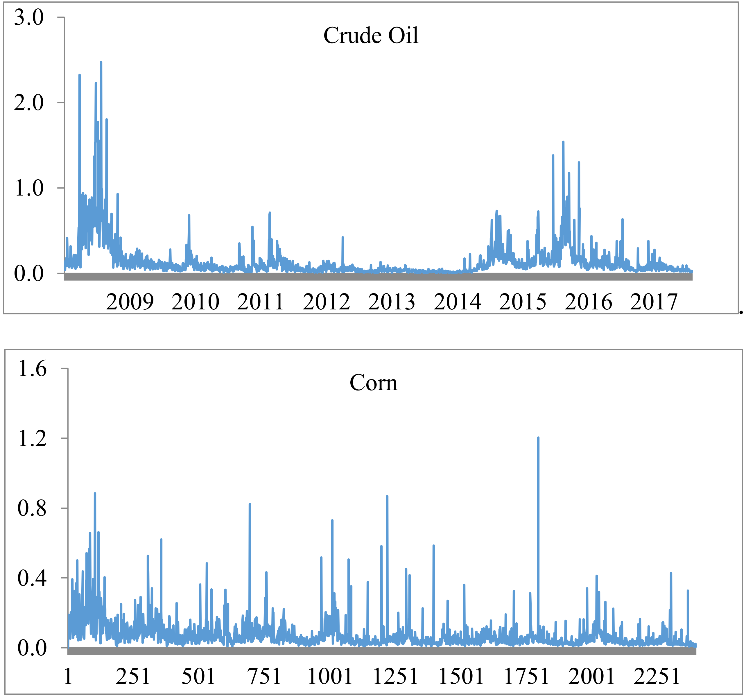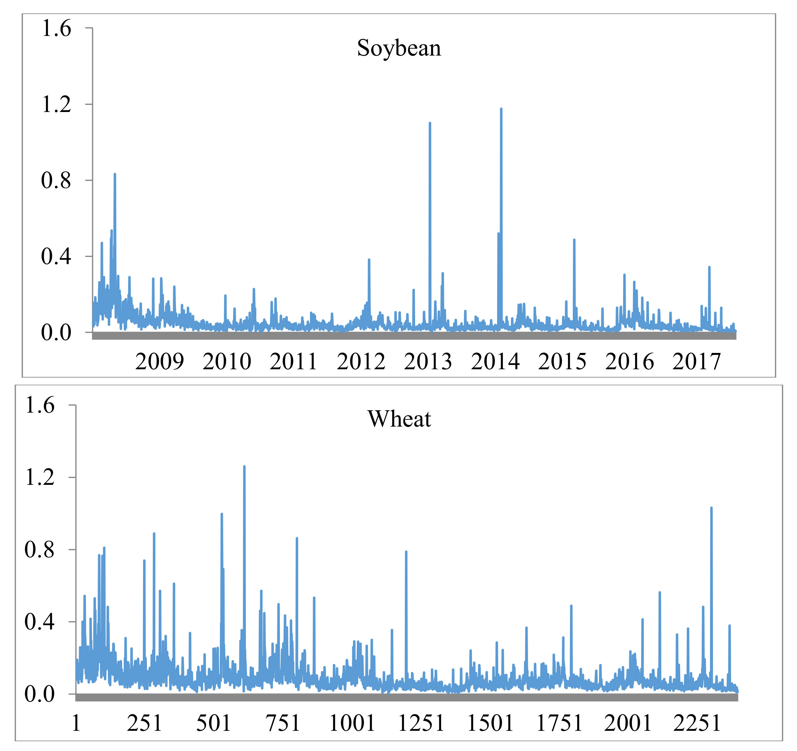Figure 1 presents the development of realized volatilities for the four commodities being analyzed. All of the series exhibited the widely-documented volatility clustering effect. A high volatility during the crisis period was observed for each of the four commodities.

3. Results

The presence of potential structural breaks implies that the volatility linkages among commodity markets may experience different features in their dynamics. To identify structural breaks, we used the Quandt–Andrews breakpoint test, which is a test for one or more unknown structural breakpoints in the sample for a specified equation. Quandt [25] generalized the Chow method to test for an unknown breakpoint by considering the F-statistic with the largest value over all possible breakdates. Andrews [26] derived the limiting distribution of the Quandt and related test statistics. Given that each bivariate HAR model contains crude oil, we tested for Equation (5) when the dependent variable was crude oil prices, and found that a break point exists on 8 December 2009. The financial crisis is often assumed to have ended in December 2009. (Friedrich [27] also regarded the fourth quarter of 2009 as the starting point of the post-crisis period when explaining puzzling global inflation dynamics.) Thus, we analyzed volatility spillovers separately for two sub-periods: the crisis period from 1 July 2008 to 7 December 2009, and the post-crisis period from 8 December 2009 to 29 December 2017. The tremendous decrease in the crude oil price started in mid-2008, which is considered to be the starting point of the 2008–09 financial crisis.

3.1. Crisis Period

The Granger causality tests (

Table 2. Granger causality tests.

	Crisis Period			Post-Crisis Period
	Corn	Soybean	Wheat	Corn	Soybean	Wheat
Oil	3.42 **	2.32 *	2.40 **	0.44	1.33	0.26
Ag.	4.41 ***	4.12 ***	4.17 ***	2.52 **	1.77	0.96

Note: This table presents the F-statistics of the Granger causality tests. The Ag. (agricultural commodity) row tested whether the agricultural commodity variable in the corresponding column caused the volatility of crude oil futures. Asterisks indicate statistical significance at the 10% (*), 5% (**), and 1% (***) levels, respectively.

) show that, in the crisis period, there were bidirectional volatility spillovers between crude oil and agricultural commodities. This bidirectional volatility spillover could very well be explained by the financialization channel. Investors sought exposure to commodity prices through speculative activity as part of a broader portfolio strategy. The effects of speculation were especially prominent before the crisis. Speculators engaged in transactions to profit from short-term market fluctuations, and paid more attention to price movements than to supply–demand fundamentals. This excessive speculation distorted prices away from the fundamental values. In this vein, the financial crisis resulted in a large outflow of investment capital from speculators for safe havens, which induced commodity markets to be subject to similar dynamics. That the price volatility in one market worried investors in other markets caused the bidirectional causality between the markets. Our finding of bidirectional volatility spillovers between crude oil and agricultural commodities is almost consistent with Nazlioglu et al. [6]. Nazlioglu et al. [6] found bidirectional volatility spillovers between oil–soybean and oil–wheat markets, but only a unidirectional volatility spillover from the oil market to the corn market. However, that volatility spills over to the oil market from the soybean and wheat markets instead of the corn market seems to make little sense, since corn is more connected with crude oil.

The estimation results from the restricted HAR models further uncover the pattern of volatility spillover (

Table 3. Estimation results of the restricted bivariate heterogeneous autoregressive (HAR) models for the crisis period.

	Oil–Corn Pair		Oil–Soybean Pair		Oil–Wheat Pair
	Oil	Corn	Oil	Soybean	Oil	Wheat
${\beta }_0$	0.19(0.08) **	−0.43(0.16) ***	0.21(0.09) **	−0.27(0.19)	0.17(0.31)	−0.37(0.15) **
${\beta }_1$		0.29(0.05) ***		0.21(0.07) ***
${\beta }_2$	0.62(0.13) ***		0.63(0.13) ***	0.42(0.12) ***	0.65(0.13) ***	0.38(0.10) ***
${\beta }_3$	0.34(0.14) **	0.53(0.08) ***	0.32(0.14) **	0.27(0.12) **	0.31(0.14) **	0.44(0.14) ***
${\beta }_4$	0.12(0.03) ***	−0.19(0.07) ***	0.11(0.03) ***	−0.15(0.07) **		−0.14(0.07) *
${\beta }_5$		0.48(0.16) ***		0.15(0.07) **	0.12(0.06) **	0.14(0.08) *
${\beta }_6$		−0.32(0.14) **
$R^2$	0.72	0.28	0.72	0.37	0.72	0.18

Note: The corresponding Newey–West standard errors are given in parentheses. Asterisks indicate statistical significance at the 10% (*), 5% (**), and 1% (***) levels, respectively.

). We observed that the short-term volatility components of corn and soybean, and the mid-term component of wheat, affected the volatility of crude oil, while other volatility components did not exhibit any impact on the volatility of crude oil. Furthermore, the magnitude of the volatility spillover of each agricultural commodity was similar. These comparable effects imply that volatility transmission might be mediated by the financialization channel when investors act in all of the commodity markets of the portfolio at the same time. However, volatility spillover effects would be more likely to be different across agricultural commodities if they were the result of the biofuel channel. Similarly, the short- and mid-term volatility components of crude oil played an important role in determining the volatility of agricultural commodities. This is consistent with the nature of speculative activities in response to short-term shocks.

3.2. Post-Crisis Period

In the post-crisis period, the Granger causality tests revealed a different picture. We only observed significant volatility spillovers from corn to crude oil prices, not the reverse. Furthermore, we did not find any volatility effects from crude oil to any of the agricultural commodities. The finding that corn volatility was unaffected by crude oil volatility via input prices can be explained by the buffer provided by government subsidies for biofuel production. While the interaction between crude oil and corn is strengthened through the biofuel production linkage, U.S. government subsidies designed to support U.S. biofuel production can actually result in corn prices being less dependent on oil prices, particularly when oil prices are at relatively low levels. Natanelov et al. [28] found that biofuel subsidies buffer the co-movement of the two markets when crude oil futures prices are below the level of $75/barrel, which was the case throughout most of the post-crisis period. Rather, the volatility spillover from corn to crude oil was a result of major events that disturbed U.S. corn production. The U.S. agriculture sector entered 2012 with corn stocks already low, followed by a severe drought in the 2012–13 production season that lowered corn stocks even further. The low stocks during this period led to corn prices exceeding $8 per bushel. High corn prices increased the cost of producing ethanol under the biofuels mandate, and pushed up the crude oil price through biofuel substitution effects.

The estimation results of the restricted HAR models reported in

Table 4. Estimation results of the restricted bivariate HAR models for the post-crisis period.

	Oil–Corn Pair		Oil–Soybean Pair		Oil–Wheat Pair
	Oil	Corn	Oil	Soybean	Oil	Wheat
${\beta }_0$	−0.08(0.08)	−0.37(0.09) ***	−0.11(0.04) ***	−0.46(0.10) ***	−0.11(0.04) ***	−0.28(0.08) ***
${\beta }_1$	0.24(0.03) ***	0.18(0.03) ***	0.25(0.03) ***	0.11(0.03) ***	0.25(0.03) ***	0.16(0.03) ***
${\beta }_2$	0.48(0.05) ***	0.34(0.05) ***	0.50(0.05) ***	0.44(0.06) ***	0.50(0.05) ***	0.38(0.05) ***
${\beta }_3$	0.24(0.04) ***	0.36(0.06) ***	0.21(0.04) ***	0.32(0.06) ***	0.21(0.04) ***	0.36(0.05) ***
${\beta }_4$
${\beta }_5$	0.11(0.04) ***
${\beta }_6$	−0.10(0.05) **
$R^2$	0.71	0.35	0.71	0.33	0.71	0.40

Note: The corresponding Newey-West standard errors are given in parentheses. Asterisks indicate statistical significance at the 10% (*), 5% (**), and 1% (***) levels, respectively.

show that both the mid-term and long-term volatility components of corn have affected the current volatility of crude oil, which is in line with the time horizons of the shocks from the 2012–13 drought. Overall, the results for the equations (Table 4) reveal that during the post-crisis period, the volatilities of all four commodities chiefly reflected their own history. The lack of effects from neighboring markets might be a sign of less speculative effects on commodity markets. Additionally, crude oil’s own short-term volatility component played a significant role, which was different from that observed during the crisis period. We also observed a decline in the importance of both the mid-term and long-term own volatility components of crude oil relative to the crisis period. As for the corn volatility equation, we found that among its own volatility components, the mid-term and long-term volatility components had comparable impacts in terms of magnitude, followed by the short-term component. In contrast, we observed no effect of the mid-term volatility component on the present volatility of corn during the crisis period. The case of soybean was similar during and after the crisis. The mid-term component played the most significant role in explaining the current volatility. Finally, the results for the wheat equation reveal a statistically significant impact of its own mid-term and long-term volatility components. The effect corresponding to the short-term component of wheat, which had no impact during the crisis period, is relatively small but positive.

3.3. Robustness Checks

The consistency of the realized volatility estimator hinges on the observability of the true (or efficient) price process. However, it is well known that a host of market microstructure effects, such as price discreteness and separate trading prices for buyers and sellers, may contaminate the true price process, and consequently, the true return data. If that occurs, the realized volatility will be a biased and inconsistent estimator of the unobservable volatility. To investigate the robustness of our findings based on five-minute returns with respect to this issue, we re-estimated our model with realized volatilities constructed from kernel-based estimators [29]. The kernel-based approach uses the first-order autocorrelation to bias correct the realized volatility, that is:

$$R{V}_t={{\displaystyle \sum }}_{i=1}^I{r}_{t,i}^2+{{\displaystyle \sum }}_{i=1}^{I-1}{r}_{t,i}{r}_{t,i+1}.$$

(6)

Hansen and Lunde [29] compared this measure to the standard measure of realized volatility (Equation (2)), and found a substantial improvement in precision under the independent noise assumption.

As seen in

Table 5. Granger causality tests for the alternative realized volatility.

	Crisis Period			Post-Crisis Period
	Corn	Soybean	Wheat	Corn	Soybean	Wheat
Oil	3.00 **	2.21 *	2.22 *	0.51	1.08	0.23
Ag.	3.30 **	4.10 ***	4.65 ***	2.78 **	1.45	1.39

Note: This table presents the F-statistics of the Granger causality tests. The Ag. (agricultural commodity) row tested whether the agricultural commodity variable in the corresponding column caused the volatility of crude oil futures. Asterisks indicate statistical significance at the 10% (*), 5% (**), and 1% (***) levels, respectively.

, the Granger causality test results were all largely unaffected. This supports the finding that there were bidirectional volatility spillovers between crude oil and agricultural commodity markets during the crisis period, while there existed only unidirectional volatility spillovers from corn to crude oil during the post-crisis period.

Table 6. Estimation results using the alternative realized volatility for the crisis period.

	Oil–Corn Pair		Oil–Soybean Pair		Oil–Wheat Pair
	Oil	Corn	Oil	Soybean	Oil	Wheat
${\beta }_0$	0.12(0.09)	−0.50(0.18) ***	0.17(0.10) *	−0.27(0.21)	0.15(0.13)	−0.38(0.19) **
${\beta }_1$		0.23(0.06) ***		0.25(0.06) ***		0.12(0.07) *
${\beta }_2$	0.65(0.14) ***		0.64(0.13) ***	0.30(0.13) **	0.66(0.14) ***	0.26(0.11) **
${\beta }_3$	0.31(0.15) **	0.56(0.08) ***	0.31(0.14) **	0.35(0.13) ***	0.30(0.15) **	0.44(0.13) ***
${\beta }_4$	0.08(0.03) ***	−0.19(0.07) ***	0.10(0.03) ***	−0.15(0.07) **		−0.19(0.08) **
${\beta }_5$		0.52(0.18) ***		0.15(0.07) **	0.10(0.06) *	0.19(0.09) **
${\beta }_6$		−0.36(0.16) **
$R^2$	0.71	0.24	0.71	0.35	0.71	0.19

Note: The corresponding Newey–West standard errors are given in parentheses. Asterisks indicate statistical significance at the 10% (*), 5% (**), and 1% (***) levels, respectively.

and

Table 7. Estimation results using the alternative realized volatility for the post-crisis period.

	Oil–Corn Pair		Oil–Soybean Pair		Oil–Wheat Pair
	Oil	Corn	Oil	Soybean	Oil	Wheat
${\beta }_0$	−0.09(0.08)	−0.37(0.10) ***	−0.12(0.04) ***	−0.48(0.11) ***	−0.12(0.04) ***	−0.31(0.09) ***
${\beta }_1$	0.22(0.03) ***	0.18(0.03) ***	0.22(0.03) ***	0.12(0.03) ***	0.22(0.03) ***	0.15(0.03) ***
${\beta }_2$	0.49(0.05) ***	0.32(0.05) ***	0.51(0.05) ***	0.42(0.06) ***	0.51(0.05) ***	0.39(0.05) ***
${\beta }_3$	0.25(0.04) ***	0.39(0.06) ***	0.22(0.04) ***	0.33(0.06) ***	0.22(0.04) ***	0.36(0.05) ***
${\beta }_4$
${\beta }_5$	0.11(0.04) ***
${\beta }_6$	−0.10(0.04) **
$R^2$	0.70	0.35	0.69	0.32	0.69	0.37

Note: The corresponding Newey–West standard errors are given in parentheses. Asterisks indicate statistical significance at the 10% (*), 5% (**), and 1% (***) levels, respectively.

present the estimation results of the restricted bivariate HAR models for both periods. The sign and significance of the parameter estimates are qualitatively and quantitatively very similar to the previous findings, and the $R^2$s for the overall goodness-of-fit of the models are also remarkably close. The only difference is that the own short-term volatility component of wheat contributed to the present volatility of wheat during the crisis period. Nonetheless, overall, the results clearly confirm the robustness of our previous findings with respect to the estimator of the realized volatility.

4. Conclusions

Volatility spillovers are a temporal concept. This study investigated the nature and dynamics of volatility spillovers between crude oil and three selected agricultural commodity markets (corn, soybean, and wheat) since the 2008–09 financial crisis. The assessment was conducted using a bivariate extension of the HAR model for the two sub-periods: the 2008–09 crisis period and the post-crisis period. The realized volatility estimator was used to measure price variation. The realized volatility based on intraday data covered a substantially larger extent of the underlying price process, and subsumed a more comprehensive information set than returns sampled at a daily or lower frequency. Therefore, the use of an advanced volatility measure ensured a far more precise analysis of the potential spillover patterns. In addition, we have contributed to the existing literature on the links between U.S. crude oil and agricultural commodity markets by using the Granger causality tests. The HAR model was used to identify the spillover effects between markets. More importantly, this methodology was able to reveal the role of volatility components established over different time periods, which cannot be done by means of the widely established GARCH framework and its variations. Moreover, this method contributed to investigating the changes of spillover patterns and identifying channels through which the changes are caused.

Our results show that the volatility relationship between crude oil and agricultural commodities has changed greatly over time. In the crisis period, there were bidirectional volatility spillovers between crude oil and agricultural commodity markets. We link this result with the financialization of commodities. It is well known that the commodity boom and the later sharp drop in prices during the global financial crisis were accompanied by an unprecedented increase in activity among financial investors in the commodity markets. Financial investors may have to unwind their positions in one-commodity markets if sudden price drops in other markets lead them to reduce risk. Therefore, the increased presence and importance of financial investors in the commodity markets has created a channel to transmit shocks across markets. The results reveal that short-term or mid-term volatility components of each commodity in a pair play a role in the other commodity, which is consistent with the characteristics of financial investor trading. In the post-crisis period, only the mid-term and long-term volatility components of corn were transmitted to crude oil, and no spillovers existed from the crude oil market to the agricultural commodity markets. We attribute the lack of volatility spillovers from crude oil to agricultural commodities to government subsidies for biofuel production. The subsidies mitigate the signal from market demand and supply and function as a buffer for volatility transmission from crude oil markets to agricultural commodities.

After the crisis, we observed an increase in the importance of commodities’ own volatility components, suggesting that these markets were restored to domination by their own economic fundamentals. That crude oil and agricultural commodity markets have become less integrated after the 2008/09 crisis is of potential interest to a variety of economic agents, including international investors and portfolio risk managers. This provides them with an opportunity to build new diversification strategies after periods of turmoil, or they could again seek exposure to commodity prices as part of a risk-reducing portfolio strategy. A good understanding of the intensity of volatility spillovers will assist them in forecasting portfolio market risk exposures among these commodity assets. For policymakers, the dynamics of spillovers among commodity markets that we present in this study will help them develop government regulations for protecting against contagion risk and fostering market stability.