Article

Remote Sensing-Based Quantification of the Relationships between Land Use Land Cover Changes and Surface Temperature over the Lower Himalayan Region

1
Department of Environmental Sciences, COMSATS University Islamabad (CUI), Abbottabad Campus, Abbottabad 22060, Pakistan
2
Department of Civil Engineering, COMSATS University Islamabad (CUI), Abbottabad Campus, Abbottabad 22060, Pakistan
3
Department of Geomatics Engineering, Schulich School of Engineering, University of Calgary, 2500 University Dr. NW, Calgary, AB T2N 1N4, Canada
4
Spatial Sciences Discipline, School of Earth and Planetary Sciences, Curtin University, Kent St, Bentley WA 6102, Australia
*
Authors to whom correspondence should be addressed.
Sustainability 2019, 11(19), 5492; https://doi.org/10.3390/su11195492
Submission received: 22 July 2019 / Revised: 28 September 2019 / Accepted: 30 September 2019 / Published: 3 October 2019
(This article belongs to the Special Issue Modelling Land Use Change and Environmental Impact)

Abstract

:
Population growth and population inflow from other regions has caused urbanization which altered land use land cover (LULC) in the lower Himalayan regions of Pakistan. This LULC change increased the land surface temperature (LST) in the region. LULC and LST changes were assessed for the period of 1990–2017 using Landsat data and the support vector machine (SVM) method. A combined cellular automata and artificial neural network (CA-ANN) prediction model was used for simulation of LULC changes for the period of 2032 and 2047 using transition potential matrix obtained from the data years of 2002 and 2017. The accuracy of the CA-ANN model was validated using simulated and classified images of 2017 with correctness value of 70% using validation modules in QGIS. The thermal bands of Landsat images from the years 1990, 2002 and 2017 were used for LST derivation. LST acquired for this period was then modeled for 2032 and 2047 using urban indices (UI) and linear regression analysis. The SVM land cover classification results showed a 5.75% and 4.22% increase in built-up area and bare soil respectively, while vegetation declined by 9.88% during 1990–2017. The results of LST for LULC classes showed that the built-up area had the highest mean LST as compared to other classes. The future projection of LULC and LST showed that the built-up area may increase by 12.48% and 14.65% in 2032 and 2047, respectively, of the total LULC area which was ~11% in 2017. Similarly, the area with temperature above 30 °C could be 44.01% and 58.02% in 2032 and 2047, respectively, of the total study area which was 18.64% in 2017. This study identified major challenges for urban planners to mitigate the urban heat island (UHI) phenomenon. In order to address the UHI in the study area, an urban planner might focus on urban plantation and decentralization of urban areas.

1. Introduction

The land use land cover (LULC) changes have become a source of concern because of its role in reducing biodiversity and altering regional climate and creating an urban heat island (UHI) in cities [1]. Rapid urbanization caused LULC changes which increased land surface temperature (LST) [2]. The land cover indicates the biophysical properties of the land surface and land use is the anthropogenic activity placed on a specific land; due to their interconnectivity they are studied together [3]. Human migration to cities causes urbanization which brings rapid changes in the ecosystem, biodiversity and the environment [4]. Rapid urbanization has both positive and negative impacts. The benefits include additional job opportunities and better life quality. The negative impacts are environmental pollution, burden on city infrastructure and health problems. The increase in built up areas in the urban center could cause an increase in LST which could be a concern for geographers, climatologists and urban planners [5,6].
The land surface consists of vegetation, water surfaces, impervious surface materials, soil and rocks. The higher trend of land surface temperature of urban areas was due to impervious surfaces which contribute towards the formation of an urban heat island (UHI) [7]. Tropical and sub-tropical climate urban areas LST depend on LULC, where built-up areas have the highest LST in comparison with arid environments in which bare soil had the highest LST [8,9]. Urban warming increased air temperature in the Himalayan region by affecting humidity and temperature of the lower boundary layer of air [10,11]. Also, the increase in LST regimes would cause the formation of an UHI [12]. The urban areas were projected to increase as they occupied only 3% of total land cover in 1950 but expected to cover 66% by 2050 [13] globally. Such rapid urban expansions may replace vegetation with built-up areas which increases LST. This results in UHI creation in urban areas of the world [14,15,16].
Many methods and algorithms were developed for LULC modeling. The most common LULC prediction models are the Markov chain [17], cellular automata (CA) [18,19] and artificial aeural network (ANN) [20]. The Markov chain is a stochastic-based model and commonly used for short term projection of a large area [21,22,23]. The CA model is a model with set transition rules and work on the principle of a neighborhood where the current state of each cell depends on the previous one and its functionality pattern is similar to LULC [24,25,26]. The validation of the CA model is done through Kappa coefficient by comparing observed and simulated LULC map [27]. The simulation of LULC changes using a cellular regression model in the lower Himalayan region for the year 2032 and 2047 showed 84% accuracy [28]. The combination of models such as CA-Markov, CA-Stochastic and CA-ANN could predict multi-directional change and give better results as compared to previously used models because the latter only deal with one-way transitional change [29,30].
Many studies indicated the relationship between LULC and LST [25,31,32,33,34]. Some researchers studied long-term and seasonal changes in temperature in relation to urban growth [35,36]. Other studies showed the quantitative relationship between LULC and temperatures without future temperature prediction [37,38,39]. The relationship between LST and a variety of LULC indices were known to be strong. Therefore, LULC indices such as normalized difference built-up index (NDBI) and fractional vegetation cover can be used for future LST projection. However only a few researchers used LULC indices for future LST projection.
Although strong correlation between LST and LULC indices were reported in several studies, only a few researchers used LULC indices for LST projection. For example, normalized difference vegetation index (NDVI) was used for simulation of urban LULC indices and LST in Dhaka Bangladesh [40]. It was reported that NDVI is not a good predictor of LST in comparison to NDBI and the percentage of impervious surface area (ISA) [32,41]. The combination of indices such as normalized difference bareness index (NDBaI), soil adjusted vegetation index, NDBI, NDVI, urban index (UI), water index, bareness index and enhanced built-up was also used for LST projection [42]. The results showed that a combination of indices in regression analysis affected model predication accuracy due to multicollinearity [40]. Several indices which included both vegetation and non-vegetation were used for LST prediction and it was found that the UI is a better predictor of LST as compared to other indices [43].
There was huge influx of population in the study area from the neighboring districts in the past three decades which caused LULC changes. Therefore, it was important to detect the past patterns of LULC and LST in this region and predict the future changes for a proper urban planning and natural resource management. This study was designed to estimate the current and future LULC and LST using a combination of remote sensing data, urban indices, modeling techniques and linear regression methods. The specific objectives of this study were to: (i) assess LULC and LST changes using Landsat data and support vector machine (SVM) method, and (ii) simulate/predict the future changes in LULC and LST regimes using the CA-ANN model and indices-based regression analysis, respectively, for the years 2032 and 2047.

2. Materials and Methods

2.1. Study Area

This study considers parts of Mansehra and Battagram districts (Figure 1) situated in Northern Pakistan, at 34°15′ to 34°45′ N latitude and 72°45′ to 73°20′ E longitude. It is located in the lower Himalayan region on the route of the China–Pakistan Economic Corridor. It has a total area of 1802 km² with a population of 1.8 million [44]. According to Köppen and Geiger, the climate of the study area is classified as Cfa which is humid subtropical or mild temperate climate [45]. The mean annual temperature is 18.5 °C and the total amount of annual rainfall is 1445 mm [46]. The study area is a tourist spot and works as a transit point to Northern Pakistan. The Karakoram Highway (KKH; Figure 1) passes through this region, which was a part of the famous ancient silk road. The people migrated from earthquake-affected districts and Afghanistan due to the Soviet–Afghan War. This migration brought significant LULC changes in the study area.

2.2. Data

In this study, three Landsat images available from the United States Geological Survey were used during 1990, 2002 and 2017 (see Table 1 for details) for evaluating changes in LULC and LST regimes. The entire Landsat scene cloud cover for the years of 1990, 2002 and 2017 was about 1%–13% but it was less than 1% in the study area (Table 1). Before LULC classification, a pretreatment process was applied in order to remove the atmospheric effects from Landsat images [47]. For LULC classification accuracy, a ground survey was conducted to collect 40 points for each land cover class. The classification accuracy was above 90% for all three classified images. The spatial variables data for LULC simulation such as road shape file and DEM was collected from local administration and the United States Geological Survey online data portal.

2.3. Methods

2.3.1. Classification Schema for LULC and Assessment of Its Accuracy

The Anderson classification scheme (Level 1) was used for LULC classification which is a commonly used classification system for Landsat data [48,49]. The acquired Landsat images were classified for the years of 1990, 2002, and 2017 using the SVM method [50,51] to generate the following land cover target classes: (i) build-up (consisting of industrial, residential, commercial infrastructure, and transportation networks); (ii) bare soil (fallow land, sand, and vacant land); (iii) vegetation (parks, trees, grasslands, and playgrounds); and (iv) water body (coastal water, lakes, canals, and streams). In order to evaluate the classification accuracy, ground truth data was obtained from the 40 land cover reference points for validation and these were overlaid on high resolution satellite images of Google Earth. For better accuracy both spectral and spatial profiles and ancillary information such as Google Earth images were used for training site development. The accuracy of the classification was assessed with kappa coefficient and overall accuracy was obtained using a confusion matrix which is a widely used method for classification accuracy [52].

2.3.2. Estimation of LST

The LST was derived from geometrically corrected Landsat satellite images for the years of 1990, 2002 and 2017. The following set of equations was used for LST calculation [53]. Firstly, the pixel-specific digital number (DN) was transformed into the radiance (Lλ) as follows:
L λ = L m a x λ L m i n λ 255 D N + L m i n λ
where Lmaxλ and Lminλ are the maximum and minimum radiance values, respectively; and their values were available from the metadata of the Landsat images. Secondly, the Lλ values were converted into brightness temperature (TB) as follows:
T B = K 2 l n K 1 L λ + 1 273.15
where K1 and K2 are constant and available from the United States Geological Survey. Thirdly, the TB values were translated into LST as follows:
L S T = T B 1 + λ   T B   σ h   c   l n ε
where λ is the center of the wavelength, σ is the Boltzmann constant (= 1.380 649 × 10−23 J/K), h is the Planck’s constant (= 6.626 × 10⁻³⁴ J/s), c is the velocity of light (= 2.998 × 10⁸ m/s), and ε is the emissivity that is being derived as follows [54]:
ε = 0.004   P V + 0.986
where PV is the proportion of vegetation and calculated as a function of NDVI values as follows:
P V = N D V I N D V I m i n N D V I m a x N D V I m i n 2
where NDVImax and NDVImin are the image-specific maximum and minimum of the NDVI values, respectively. Also, the calculation of NDVI is found in Table 2.
Note that the Landsat 8 has two thermal bands centered at 10.9 µm and 12 µm. Therefore, LST for Landsat 8 was calculated by averaging LST values from both of the bands.

2.3.3. Normalization of LST

As the LST images were generated for three different years, normalizing them prior to further analysis was required. The LST image of 2017 was used as the reference in this normalization process. The z-score method was employed for this purpose with the following expression as modified after Salama et al. [55]:
L S T n j = L S T j L S T j ¯ L S T σ j L S T σ i + L S T i ¯
where L S T n j is the pixel-specific normalized LST values for the year j (= 1990 or 2002); L S T j is the pixel-specific LST values in the original image prior to normalization; L S T j ¯ is the image-specific average LST values for either 1990 or 2002; L S T σ j is the image-specific standard deviation of the LST values for either 1990 or 2002; L S T σ i is the image-specific standard deviation of the LST values for the reference year i (= 2017); and L S T i ¯ is the image-specific average LST value for 2017.
Upon execution of the above-mentioned normalization, LST values were classified into six target categories as: (i) <15, (ii) 15 to <21, (iii) 21 to <24, (iv) 24 to <27, (v) 27 to <30 and (vi) ≥30 °C. Subsequently, calculations were done to determine the proportion of areas under each of these categories. Such analysis, in fact, evaluated the temporal variability/trends in each LST categories.

2.3.4. Modeling of LULC Changes for 2032 and 2047

Several prediction models were employed previously for modeling the future LULC [56]. In the current study, modeling of LULC changes for 2032 and 2047 was completed using a combined CA-ANN model in QGIS. It first modeled the transition potential matrix using ANN, then predicted future LULC changes using the CA model. A combination of models such as CA and ANN (CA-ANN) can predict multi-directional change and give better results than the models which deal only with one-way transitional change [29,30]. The LULC for the years 2032 and 2047 was predicted using the 2002 and 2017 year-specific classified images. A similar method was used by [57] for prediction of LULC for the year 2028 using classified images from 2002 and 2015 in the Coastal Assasuni Upazila area in south-western Bangladesh. Variables of elevation and distance from main roads were used as land use dynamics or drivers. The land use drivers and classified images from 2002 and 2017 were used to generate a transition potential matrix using the QGIS MOLUSCE tool. Once the transition potential matrix was generated then this was modeled using ANN. Finally, LULC projection for 2032 and 2047 was obtained by the CA model. The validation of the CA-ANN model is important; therefore, the CA-ANN model was validated by comparing simulated LULC for 2017 with estimated LULC of 2017 using MOLUSCE QGIS validation.

2.3.5. Modeling of LST for 2032 and 2047

After simulating the LULC for 2032 and 2047, the LULC indices-based methodology proposed by [43] was modified in this study to project LST for the years 2032 and 2047. The different indices which were used for forecasting LST change were NDBaI, NDVI, NDBI and UI. The indices-specific equations are provided in Table 2.
After derivation of LULC indices, correlation (bivariate) analysis between indices and LST was performed in order to select the indices that had strong correlation with LST. The correlation analysis between indices and LST showed that the UI significantly correlated with LST (p < 0.05). The values of correlation coefficient (R) and Root Mean Square Error (RMSE) were 0.410 and 0.094, respectively. A regression model with a selected index (i.e., UI), was then used to project the LST for 2032 and 2047. The regression analysis was conducted between UI and LST in order to formulate the regression equation. The following regression equation was formulated using UI and LST from the year 2017.
LST = 24.25 + (12.41 UI)
Since the CA-ANN model determines classes, thus UI indices were recategorized so that they could determine <15, 15 to <21, 21 to <24, 24 to <27, 27 to 30 and ≥30 °C surface temperature classes. The selected UI indices from 2002 and 2017 were simulated using the CA-ANN to project their changes in 2032 and 2047. Finally, Equation (6) and predicted/simulated UI indices were employed to calculate LST for the years 2032 and 2047.

3. Results

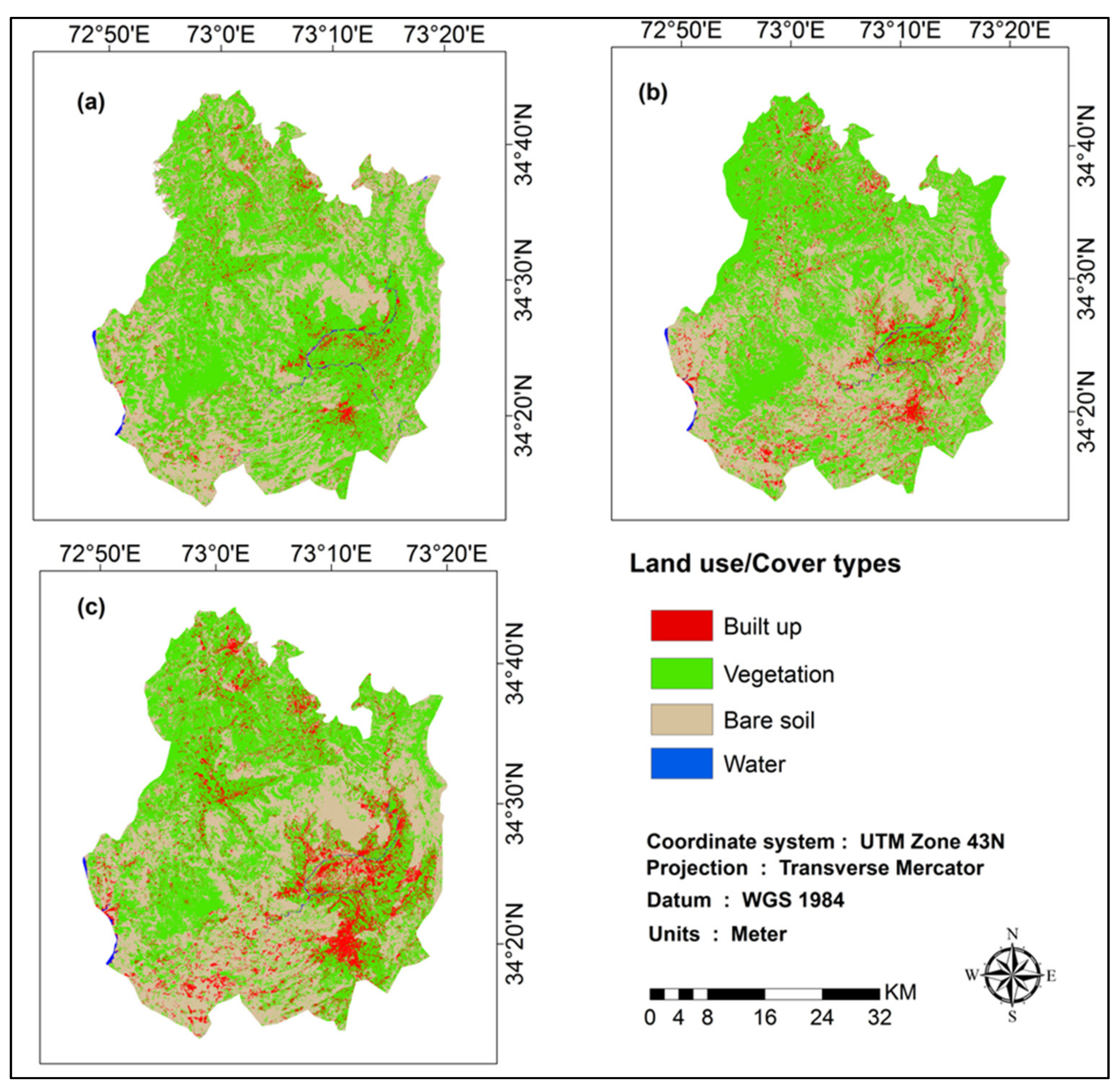
3.1. Past Pattern of LULC Classes

LULC maps were classified using the SVM method, and its accuracy was evaluated by kappa coefficient using the confusion matrix (see Table 3 for details). The kappa coefficient value was above 0.87 for all three classified images. The overall classification accuracy was 94.96%, 92.26% and 91.35% for the years of 1990, 2002 and 2017, respectively (Table 3). The results are given in Figure 2 and Table 4. The outcomes indicated that most of the built-up area increase happened in the urban parts of the districts of Mansehra and Battagram (Figure 2). The built-up area increased from 5.75% to 10.87% of total area during the period of 1990–2017 (Table 4). Table 4 indicated that vegetation declined significantly by 175.77 km2 (−9.88%) during the study period. The built-up area was expanded by 103.87 km2 (5.75%). The amount of bare soil increased by 77.8 km2 (4.22%) from the year of 1990 to 2017.

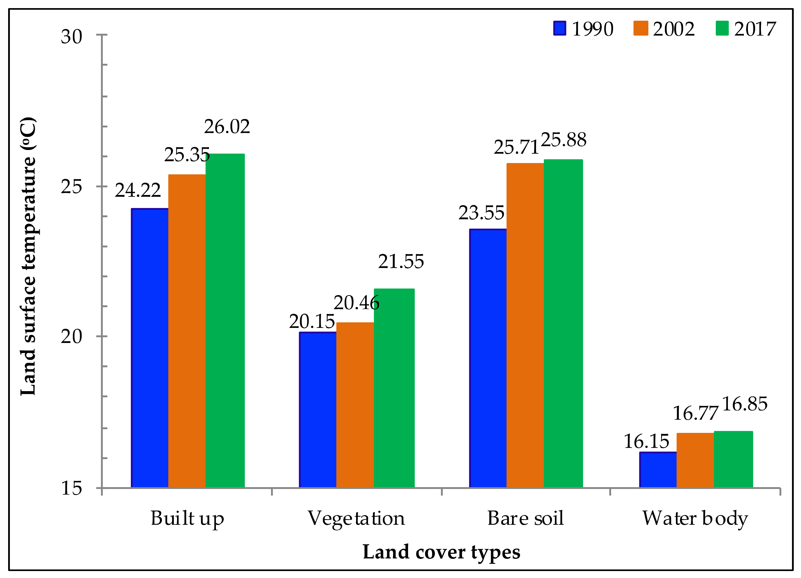
3.2. Past Pattern of LST

The mean LST of individual LULC classes are given in Figure 3. Overall its trend from higher to lower range was for built-up, bare soil, vegetation and water body. The mean LST for built-up areas expanded from 24.22 °C to 26 °C during the 1990‒2017 period. Similarly, LST for vegetation and bare soil increased from 20.15 °C to 21.55 °C and 23.5 °C to 25.8 °C, respectively, during this period. The mean LST for water body increased from 16.15 °C to 16.85 °C during the same data period. When the average decadal temperature per class was examined, there was a significant temperature increase (by ~1 °C) from 2002 to 2017 for the built-up area. A similar trend was observed for vegetation, bare soil and water body.
The areal distribution of LST among the different temperature ranges for 1990, 2002 and 2017 is given in Figure 4. The results indicated that in 1990 only 0.8% area had a temperature above 30 °C which increased to 18.64% in 2017. The LST increased from 10.53% to 16.54% for the temperature of 27 °C to 30 °C. The decreasing trend was observed for temperature below 24 °C. For example, the temperature ranged from 21 °C to 24 °C decreased from 31.52% to 20.04%. A similar trend was observed with temperature range of 15 °C to 21 °C. The increase in LST from 2002 to 2017 was greater than from 1990 to 2002. The spatial distribution of the LST in the study area for 1990, 2002 and 2017 is given in Figure 5. It showed that high temperature regimes were mostly found in the urban area (Tehsil Mansehra) as compared to sub-urban area such as Oghi and Battagram (Figure 1).

3.3. Modeling of LULC Changes for the Year 2032 and 2047

Figure 6 demonstrates the simulated/predicted LULC patterns for the years 2032 and 2047 and areal statistics are given in Table 5. The accuracy of the CA-ANN model showed %-correctness value of 70% which is an acceptable accuracy level. The results showed that the total built-up area could be ~12.5% and ~15% in 2032 and 2047, respectively, which was ~11% in 2017. The projected results indicated that vegetation could be 45.03% and 42.61% in 2032 and 2047, respectively, which was ~47% in 2017. The bare soil could change to almost 42.35% and 42.63% of the total area in 2032 and 2047, respectively, which was 42.14% in 2017. The bare soil showed an increasing trend for the projected time period. There was no significant change in water body from the base year of 2017. The water content will be 0.12% and 0.08% in 2032 and 2047, respectively, which was 0.23% of the total land cover in 2017.

3.4. Modeling of LST Changes for the Years 2032 and 2047

Figure 7 shows the simulated LST for 2032 and 2047 and areal statistics are provided in Table 6. The LST range above 30 °C was 44.01% and 58.02% in 2032 and 2047, respectively, which was 18.64% in 2017. The mean LST for 2032 and 2047 was above 30 °C for the study area which was 18.64 °C in 2017. The results indicated that the area in the LST range less than 30 °C decreased while above 30 °C showed an increasing trend in the modeling forecast.

4. Discussions

4.1. Change in LULC

The current research study examined LULC changes during the 1990‒2017 period. The results indicated a 2.31% increase in built-up area from 2002 and 2017. The built-up area was increased by 5.75% from 1990 to 2017. The built-up and bare soil increased at the expense of vegetation which declined by −9.98% during the 1990‒2002 period, and the built-up area expanded from 93.11 km2 to 134.85 km2 which was less as compared to the built-up during the period of 2002–2017. Similar decadal growth was noted in other South Asian cities such as Kathmandu [61] and Dhaka [62]. Several factors contributed to urbanization such as population growth, the political and economic situation, and the migration of people from surrounding areas especially Balakot after the 2005 earthquake [63]. The natural increase in Pakistan’s general population could also be a major reason for urbanization. The population of Pakistan has been growing by 2% on a yearly basis (four children per mother); if this remains constant, Pakistan’s population could be nearly 300 million by 2030, and 450 million by 2050. The Soviet–Afghan War from 1979‒1989 in Afghanistan led to a massive influx of migrants from across the border into urban areas of Pakistan. Nearly four million Afghans migrated into north-western Pakistan during the Soviet–Afghan War. Initially they settled in border refugee camps, but later on they migrated into cities. As suggested by different authors, a combination of political and economic factors [64] and high population growth rate [65] were the major reasons for the urban growth in general, with our study area as not an exception, but rather a hot spot. These factors caused a speedy growth of urban areas and a combination of urban and rural LULC categories became the key features in our area of interest. The newly built-up areas were more frequently witnessed, specifically in the sub-urban zones. Built-up areas and bare soil mostly replaced the areas previously covered by vegetation but located at a lower altitude near the built-up areas.

4.2. Change in LST

Our study found that built-up areas had the highest land surface temperature followed by bare soil, vegetation and water. Similar findings were reported by [64] who assessed the LULC impact on the land surface temperature in Zhujiang (China), in order to assess LULC and thermal signature relationship. These outcomes were similar to [66], who found that bare soil and built-up area had a higher LST as compared to water bodies and vegetation categories. The current study showed that the LST regimes expanded due to conversion of vegetative surfaces into non-vegetated areas. The findings of the current study also indicated that LST increased for all LULC classes from 1990 to 2017 (Figure 3 and Figure 5) which was probably due to global warming and surface modification. According to Terando et al. [67], LST could increase when urban expansion cascaded with climate change [68]. Similar findings in the lower Himalayan region were also reported [28]. The increase in LST in the study area was higher due to speedy urbanization from 1990 to 2017. Another fact, such as different temporal resolution of Landsat images could contribute for the LST increase beyond the built-up area; however, the outcomes showed that the area was affected by both local warming and/or climate change.

4.3. Modeling of LULC Changes for the Year 2032 and 2047

The LULC of the study area is expected to change over the next three decades, as 12.48% and 14.65% of the current land use land cover could be transformed into a built-up class in 2032 and 2047, respectively, which was 10.87% in 2017. A similar trend of built-up areas was also noticed in future forecasting for other growing cities, like Beijing in China [69]. The increasing built-up areas might be associated with the population growth during different decades since 1990, as found in the case of Bangladesh [70]. Rapid urbanization creates an urban sprawl which has both positive and negative impacts. The positive impacts include industrialization which increases employment opportunities to local residents and others living in the surrounding areas. The urban expansion could increase business opportunities and improve health facilities. The construction and establishment of new housing societies could increase in the study area as well. The construction of new luxurious residential societies could provide comfortable and improved living standards to people.
Some of the negative impacts of urbanization include unemployment, extra fuel consumption and several health- and environment-related issues. With the growing population, there is an increasing need of employment opportunities as Pakistan’s population is projected to be 306 million in 2050, which could be 3.6% of the total world population [71]. Similarly, the population increase and city expansion increases traveling distance for residences which may cause additional fuel usage and traffic jams. It could increase air pollution and impact numerous health-related issues, especially for the children and the senior citizens in our area of interest. This could also increase pressure on public services. Urbanization also causes social disparities among residents [72].

4.4. Modeling of LST Changes for the Year 2032 and 2047

The LST modeled in this study for 2032 and 2047 demonstrated that the LST regimes could be over 27 °C for most of the study area. The predicted temperature increase due to rapid urban growth concurs with the variety of regional and global models which predicted similar scenarios for urban growth [73,74,75]. This is due to high energy demands caused by population increase. The urban expansion effects greenhouse gases which are mostly released from different human activities. In fact, enormous amounts of anthropogenic carbon dioxide emissions are usually the case in urban areas as a result of burning of fossil fuels for: (i) both cooling and heating; (ii) industrial production; (iii) vehicles. For example, Kahn [76] noted that the greenhouse gas concentration and anthropogenic heat emissions could intensify due to urbanization as the population may grow in the middle class. The income increment in the middle class could raise the consumption of gadgets such as air conditioners, fridges, stoves and heaters. Forest work as a major carbon sink which was affected by LULC changes primarily by deforestation at the regional scale, caused changes in surface characteristics which could be the reason for an increase in LST along with other factors such as land utilization for roads and cities and goods and services demands by urban residents [77]. The mean annual temperature in Pakistan has increased by 0.57 °C during the past 100 years and it will further increase by 3 °C to 5 °C as per central global emissions scenario, while as per higher global emissions scenario, it will rise by 4 °C to 6 °C [78]. Since air temperature and LST are correlated, therefore an increase in air temperature would lead to an increase in LST and land surface temperature would be greater than air temperature [79]. The increase in temperature could have negative impacts on plants and animal species as well as human health.

5. Conclusions

The main purpose of this study was to assess the effect of LULC on LST during the period 1990‒2017 in the study area. Landsat data and support vector machine method were used to generate LULC classification maps. The past trends of LULC and LST were employed in CA-ANN and regression models to predict the future trends of these two variables. The results indicated significant changes in the LULC, in particular the built-up and bare soil area were amplified by 5.75% and 4.22% respectively, while vegetation declined by 9.88% during the past data period of 1990‒2017. The zonal analysis between LST and LULC indicated that the mean LST for a built-up area was high as compared to other classes. The land surface temperature increased for all land cover classes which was due to both urban warming and climate change. The future simulation results showed that the built-up area is expected to encompass 12.48% and 14.65% of the total study area in 2032 and 2047, respectively, as compared to ~11% in 2017. Similarly, the area with an LST above 30 °C could increase to ~44% and ~58% of the total area in 2032 and 2047, respectively, as compared to ~18% in 2017. It was noted that lower temperature zones are shifting towards higher temperatures which could lead to large-scale UHI formation. This study identified major challenges for urban planners to mitigate UHIs in the study area. Urban plantation and decentralization of urban areas are two possible solutions in order to mitigate the UHI and its consequences. Future urban research could focus on the issue of public health and infrastructure burden associated with rapid urbanization.

Author Contributions

Conceptualization, S.U. and A.A.T.; formal analysis, S.U., A.A.T., T.A.A., A.J.K. and M.K.; methodology, S.U., A.A.T., T.A.A., Q.K.H., A.D. and M.K.; validation, A.A.T.; writing—original draft, S.U., A.A.T., T.A.A. and Q.K.H.; writing—review and editing, A.D., A.J.K. and M.K.

Funding

This research received no external funding.

Acknowledgments

The authors would like to thank the United States Geological Survey for providing satellite data.

Conflicts of Interest

The authors have no conflicts of interest.

References

  1. Aguilar, A.G.; Ward, P. Globalization, regional development, and mega-city expansion in Latin America: Analyzing Mexico City’s peri-urban hinterland. Cities 2003, 20, 3–21. [Google Scholar] [CrossRef]
  2. Yuen, B.; Kong, L. Climate change and urban planning in Southeast Asia. SAPI EN. S. Surv. Perspect. Integr. Environ. Soc. 2009, 2, 3. [Google Scholar]
  3. Verburg, P.H.; Van De Steeg, J.; Veldkamp, A.; Willemen, L. From land cover change to land function dynamics: A major challenge to improve land characterization. J. Environ. Manag. 2009, 90, 1327–1335. [Google Scholar] [CrossRef] [PubMed]
  4. Uttara, S.; Elliot, S. Impacts of urbanization on environment. Int. J. Res. Eng. Appl. Sci. 2012, 2, 1637–1645. [Google Scholar]
  5. Maimaitiyiming, M.; Ghulam, A.; Tiyip, T.; Pla, F.; Latorre-Carmona, P.; Halik, Ü.; Sawut, M.; Caetano, M. Effects of green space spatial pattern on land surface temperature: Implications for sustainable urban planning and climate change adaptation. ISPRS J. Photogramm. Remote Sens. 2014, 89, 59–66. [Google Scholar] [CrossRef] [Green Version]
  6. Gaffin, S.R.; Rosenzweig, C.; Khanbilvardi, R.; Parshall, L.; Mahani, S.; Glickman, H.; Goldberg, R.; Blake, R.; Slosberg, R.B.; Hillel, D. Variations in New York city’s urban heat island strength over time and space. Theor. Appl. Climatol. 2008, 94, 1–11. [Google Scholar] [CrossRef]
  7. Zhang, Y.; Balzter, H.; Liu, B.; Chen, Y. Analyzing the impacts of urbanization and seasonal variation on land surface temperature based on subpixel fractional covers using Landsat images. IEEE. J. Sel. Top. Appl. Earth Obs. Remote Sens. 2017, 10, 1344–1356. [Google Scholar] [CrossRef]
  8. Xiao, R.B.; Weng, Q.H.; Ouyang, Z.Y.; Li, W.F.; Schienke, E.W.; Zhang, Z.M. Land surface temperature variation and major factors in Beijing, China. Photogramm. Eng. Remote Sens. 2008, 74, 451–461. [Google Scholar] [CrossRef]
  9. Li, X.; Zhou, W.; Ouyang, Z.; Xu, W.; Zheng, H. Spatial pattern of greenspace affects land surface temperature: Evidence from the heavily urbanized Beijing metropolitan area, China. Landsc. Ecol. 2012, 27, 887–898. [Google Scholar] [CrossRef]
  10. Boos, W.R.; Kuang, Z. Dominant control of the south Asian monsoon by orographic insulation versus plateau heating. Nature 2010, 463, 218. [Google Scholar] [CrossRef] [PubMed]
  11. Cao, W.; Huang, L.; Liu, L.; Zhai, J.; Wu, D. Overestimating impacts of urbanization on regional temperatures in developing megacity: Beijing as an example. Adv. Meteorol. 2019, 2019, 3985715. [Google Scholar] [CrossRef]
  12. Lai, L.W.; Cheng, W.L. Urban heat island and air pollution—An emerging role for hospital respiratory admissions in an urban area. J. Environ. Health 2010, 72, 32–35. [Google Scholar] [PubMed]
  13. United Nations, Department of Economic and Social Affairs. P.D. World Urbanization Prospects: The 2018 Revision; United Nations, Department of Economic and Social Affairs: New York, NY, USA, 2018. [Google Scholar]
  14. Yang, C.; He, X.; Yan, F.; Yu, L.; Bu, K.; Yang, J.; Chang, L.; Zhang, S. Mapping the influence of land use/land cover changes on the urban heat island effect—A case study of Changchun, China. Sustainability 2017, 9, 312. [Google Scholar] [CrossRef]
  15. Ahmed, S. Assessment of urban heat islands and impact of climate change on socioeconomic over Suez governorate using remote sensing and GIS techniques. Egypt. J. Remote Sens. Space Sci. 2018, 21, 15–25. [Google Scholar] [CrossRef]
  16. Balzter, H. Markov chain models for vegetation dynamics. Ecol. Model. 2000, 126, 139–154. [Google Scholar] [CrossRef] [Green Version]
  17. Santé, I.; García, A.M.; Miranda, D.; Crecente, R. Cellular automata models for the simulation of real-world urban processes: A review and analysis. Landsc. Urban Plan. 2010, 96, 108–122. [Google Scholar] [CrossRef]
  18. Zenil, H. Compression-based investigation of the dynamical properties of cellular automata and other systems. arXiv 2009, arXiv:0910.4042. [Google Scholar]
  19. Civco, D.L. Artificial neural networks for land-cover classification and mapping. Int. J. Geogr. Inf. Sci. 1993, 7, 173–186. [Google Scholar] [CrossRef]
  20. Agarwal, C.; Green, G.M.; Grove, J.M.; Evans, T.P.; Schweik, C.M. A Review and Assessment of Land-Use Change Models: Dynamics of Space, Time, and Human Choice; Gen. Tech. Rep. NE-297; Newton Square, U.S. Department of Agriculture, Forest Service, Northeastern Research Station: Washington, DC, USA, 2002; 61p. [Google Scholar]
  21. Weng, Q. Land use change analysis in the Zhujiang Delta of China using satellite remote sensing, GIS and stochastic modelling. J. Environ. Manag. 2002, 64, 273–284. [Google Scholar] [CrossRef] [Green Version]
  22. Kumar, S.; Radhakrishnan, N.; Mathew, S. Land use change modelling using a markov model and remote sensing. Geomat. Nat. Hazards Risk 2014, 5, 145–156. [Google Scholar] [CrossRef]
  23. Parsa, V.A.; Salehi, E. Spatio-temporal analysis and simulation pattern of land use/cover changes, case study: Naghadeh, Iran. J. Urban Manag. 2016, 5, 43–51. [Google Scholar] [CrossRef] [Green Version]
  24. Hadi, S.J.; Shafri, H.Z.M.; Mahir, M.D. Modelling LULC for the period 2010–2030 using GIS and remote sensing: A case study of Tikrit, Iraq. In IOP Conference Series: Earth and Environmental Science; IOP Publishing: Bristol, UK, 2014; Volume 20, p. 12053. [Google Scholar]
  25. Rahaman, K.R.; Ahmed, M.R.; Hassan, Q.K. Using satellite-borne remote sensing data in generating local warming maps with enhanced resolution. ISPRS Int. J. Geo-Inf. 2018, 7, 398. [Google Scholar] [CrossRef]
  26. Eastman, J.R. Idrisi Taiga; Clark Labs Clark University: Worcester, MA, USA, 2009. [Google Scholar]
  27. Ullah, S.; Ahmad, K.; Sajjad, R.U.; Abbasi, A.M.; Nazeer, A.; Tahir, A.A. Analysis and simulation of land cover changes and their impacts on land surface temperature in a lower Himalayan region. J. Environ. Manag. 2019, 245, 348–357. [Google Scholar] [CrossRef] [PubMed]
  28. Guan, D.; Li, H.; Inohae, T.; Su, W.; Nagaie, T.; Hokao, K. Modeling urban land use change by the integration of cellular automaton and markov model. Ecol. Model. 2011, 222, 3761–3772. [Google Scholar] [CrossRef]
  29. Keshtkar, H.; Voigt, W. A spatiotemporal analysis of landscape change using an integrated markov chain and cellular automata models. Model. Earth Syst. Environ. 2016, 2, 10. [Google Scholar] [CrossRef]
  30. Hu, Y.; Jia, G. Influence of land use change on urban heat island derived from multi-sensor data. Int. J. Climatol. 2010, 30, 1382–1395. [Google Scholar] [CrossRef]
  31. Li, J.; Wang, X.; Wang, X.; Ma, W.; Zhang, H. Remote sensing evaluation of urban heat island and its spatial pattern of the Shanghai Metropolitan Area, China. Ecol. Complex. 2009, 6, 413–420. [Google Scholar] [CrossRef]
  32. Xu, L.Y.; Xie, X.D.; Li, S. Correlation analysis of the urban heat island effect and the spatial and temporal distribution of atmospheric particulates using TM images in Beijing. Environ. Pollut. 2013, 178, 102–114. [Google Scholar] [CrossRef]
  33. Jiang, J.; Tian, G. Analysis of the impact of land use/land cover change on land surface temperature with remote sensing. Procedia Environ. Sci. 2010, 2, 571–575. [Google Scholar] [CrossRef]
  34. Mushore, T.D.; Mutanga, O.; Odindi, J.; Dube, T. Assessing the potential of integrated Landsat 8 thermal bands, with the traditional reflective bands and derived vegetation indices in classifying urban landscapes. Geocarto Int. 2017, 32, 886–899. [Google Scholar] [CrossRef]
  35. Sung, C.Y. Mitigating surface urban heat island by a tree protection policy: A case study of the Woodland, Texas, USA. Urban Green. 2013, 12, 474–480. [Google Scholar] [CrossRef]
  36. Odindi, J.O.; Bangamwabo, V.; Mutanga, O. Assessing the value of urban green spaces in mitigating multi-seasonal urban heat using MODIS land surface temperature (LST) and Landsat 8 data. Int. J. Environ. Res. 2015, 9, 9–18. [Google Scholar]
  37. Xiao, H.; Kopecká, M.; Guo, S.; Guan, Y.; Cai, D.; Zhang, C.; Zhang, X.; Yao, W. Responses of urban land surface temperature on land cover: A comparative study of Vienna and Madrid. Sustainability 2018, 10, 260. [Google Scholar] [CrossRef]
  38. Yuan, F.; Bauer, M.E. Comparison of impervious surface area and normalized difference vegetation index as indicators of surface urban heat island effects in Landsat imagery. Remote Sens. Environ. 2007, 106, 375–386. [Google Scholar] [CrossRef]
  39. Tran, H.; Uchihama, D.; Ochi, S.; Yasuoka, Y. Assessment with satellite data of the urban heat island effects in Asian Mega Cities. Int. J. Appl. Earth Obs. Geoinf. 2006, 8, 34–48. [Google Scholar] [CrossRef]
  40. Ahmed, B.; Kamruzzaman, M.; Zhu, X.; Rahman, M.S.; Choi, K. Simulating land cover changes and their impacts on land surface temperature in Dhaka, Bangladesh. Remote Sens. 2013, 5, 5969–5998. [Google Scholar] [CrossRef]
  41. Weng, Q.; Lu, D.; Schubring, J. Estimation of land surface temperature-vegetation abundance relationship for urban heat island studies. Remote Sens. Environ. 2004, 89, 467–483. [Google Scholar] [CrossRef]
  42. Hasanlou, M.; Mostofi, N. Investigating urban heat island estimation and relation between various land cover indices in Tehran city using Landsat 8 imagery. In Proceedings of the 1st International Electronic Conference on Remote Sensing, Basel, Switzerland, 22 June–5 July 2015; pp. 1–11. [Google Scholar]
  43. Mushore, T.D.; Odindi, J.; Dube, T.; Mutanga, O. Prediction of future urban surface temperatures using medium resolution satellite data in Harare Metropolitan City, Zimbabwe. Build. Environ. 2017, 122, 397–410. [Google Scholar] [CrossRef]
  44. Pakistan Bureau of Statistics. District Wise Census Results [WWW Document]. Available online: http://www.pbscensus.gov.pk/sites/default/files/bwpsr/kp/ABBOTTABAD_SUMMARY.pdf (accessed on 20 January 2019).
  45. Kottek, M.; Grieser, J.; Beck, C.; Rudolf, B.; Rubel, F. World map of the Köppen-Geiger climate classification updated. Meteorol. Z. 2006, 15, 259–263. [Google Scholar] [CrossRef]
  46. Afzaal, M.; Haroon, M.A.; Zaman, Q. Interdecadal oscillations and the warming trend in the area-weighted annual mean temperature of Pakistan. Pak. J. Meteorol. 2009, 6, 13–19. [Google Scholar]
  47. Landsat, N. Science Data Users Handbook; NASA: Washington, DC, USA, 2019. [Google Scholar]
  48. Anderson, J.R. A Land Use and Land Cover Classification System for Use with Remote Sensor Data; US Government Printing Office: Washington, DC, USA, 1976; Volume 964.
  49. Rozenstein, O.; Karnieli, A. Comparison of methods for land-use classification incorporating remote sensing and GIS inputs. Appl. Geogr. 2011, 31, 533–544. [Google Scholar] [CrossRef]
  50. Vapnik, V.N.; Chervonenkis, A.Y. The uniform convergence of frequencies of the appearance of events to their probabilities. In Doklady Akademii Nauk; Russian Academy of Sciences: Moscow, Russia, 1968; Volume 181, pp. 781–783. [Google Scholar]
  51. Vapnik, V.N. An overview of statistical learning theory. IEEE Trans. Neural Netw. 1999, 10, 988–999. [Google Scholar] [CrossRef] [PubMed]
  52. Foody, G.M. Status of land cover classification accuracy assessment. Remote Sens. Environ. 2002, 80, 185–201. [Google Scholar] [CrossRef]
  53. Artis, D.A.; Carnahan, W.H. Survey of emissivity variability in thermography of urban areas. Remote Sens. Environ. 1982, 12, 313–329. [Google Scholar] [CrossRef]
  54. Sobrino, J.A.; Jiménez-Muñoz, J.C.; Paolini, L. Land surface temperature retrieval from Landsat TM 5. Int. J. Appl. Sci. Technol. 2004, 90, 434–440. [Google Scholar] [CrossRef]
  55. Salama, M.S.; Van der Velde, R.; Zhong, L.; Ma, Y.; Ofwono, M.; Su, Z. Decadal variations of land surface temperature anomalies observed over the Tibetan plateau by the special sensor microwave imager (SSM/I) from 1987 to 2008. Clim. Chang. 2012, 114, 769–781. [Google Scholar] [CrossRef]
  56. Triantakonstantis, D.; Mountrakis, G. Urban growth prediction: A review of computational models and human perceptions. J. Geogr. Inf. Syst. 2012, 4, 555–587. [Google Scholar] [CrossRef]
  57. Sarkar, L.; Rasheduzzaman, M.; Zahedul Islam, A.Z.M.; Tabassum, F.; Saba, H.; Uddin, S.Z.; Rahman, M.T.U.; Ferdous, J. Temporal dynamics of land use/land cover change and its prediction using CA-ANN model for southwestern coastal Bangladesh. Environ. Monit. Assess. 2017, 189, 565. [Google Scholar] [CrossRef]
  58. Chen, X.-L.; Zhao, H.-M.; Li, P.-X.; Yin, Z.-Y. Remote sensing image-based analysis of the relationship between urban heat island and land use/cover changes. Remote Sens. Environ. 2006, 104, 133–146. [Google Scholar] [CrossRef]
  59. Zha, Y.; Gao, J.; Ni, S. Use of normalized difference built-up index in automatically mapping urban areas from TM imagery. Int. J. Remote Sens. 2003, 24, 583–594. [Google Scholar] [CrossRef]
  60. Katayama, R.; Shozi, M.; Tokiya, Y. A research on the urban disaster prevention plan concerning earthquake risk forecast by remoto sensing in the Tokyo Bay Area. ISPRS 2000, B7, 669. [Google Scholar]
  61. Thapa, R.B.; Murayama, Y. Examining spatiotemporal urbanization patterns in Kathmandu Valley, Nepal: Remote sensing and spatial metrics approaches. Remote Sens. 2009, 1, 534–556. [Google Scholar] [CrossRef]
  62. Dewan, A.; Corner, R. Dhaka Megacity: Geospatial Perspectives on Urbanisation, Environment and Health; Springer Science and Business Media: Berlin, Germany, 2013. [Google Scholar]
  63. Pakistan Bureau of Statistics. Tehsil Wise Census Results [WWW Document]. Available online: http://www.pbscensus.gov.pk/sites/default/files/bwpsr/kp/ABBOTTABAD_SUMMARY.pdf (accessed on 20 January 2019).
  64. Weng, Q. A remote sensing? GIS evaluation of urban expansion and its impact on surface temperature in the Zhujiang Delta, China. Int. J. Remote Sens. 2001, 22, 1999–2014. [Google Scholar]
  65. Abou-Korin, A.A. Impacts of rapid urbanisation in the Arab World: The case of Dammam metropolitan area, Saudi Arabia. In Proceedings of the 5th International Conference and Workshop on Built Environment in Developing Countries (ICBEDC 2011), Penang, Malaysia, 6–7 December 2011; pp. 1–25. [Google Scholar]
  66. Adegoke, J.O.; Pielke, S.R.A.; Eastman, J.; Mahmood, R.; Hubbard, K.G. Impact of irrigation on midsummer surface fluxes and temperature under dry synoptic conditions: A regional atmospheric model study of the US high plains. Mon. Weather Rev. 2003, 131, 556–564. [Google Scholar] [CrossRef]
  67. Terando, A.J.; Costanza, J.; Belyea, C.; Dunn, R.R.; McKerrow, A.; Collazo, J.A. The southern megalopolis: Using the past to predict the future of urban sprawl in the Southeast US. PLoS ONE 2014, 9, e102261. [Google Scholar] [CrossRef]
  68. Ren, G.; Zhou, Y.; Chu, Z.; Zhou, J.; Zhang, A.; Guo, J.; Liu, X. Urbanization effects on observed surface air temperature trends in North China. J. Clim. 2008, 21, 1333–1348. [Google Scholar] [CrossRef]
  69. Han, H.; Yang, C.; Song, J. Scenario simulation and the prediction of land use and land cover change in Beijing, China. Sustainability 2015, 7, 4260–4279. [Google Scholar] [CrossRef]
  70. Hasan, S.; Deng, X.; Li, Z.; Chen, D. Projections of future land use in Bangladesh under the background of baseline, ecological protection and economic development. Sustainability 2017, 9, 505. [Google Scholar] [CrossRef]
  71. DESA, U.N. United Nations Department of Economic and Social Affairs/Population Division (2009b): World Population Prospects: The 2008 Revision. Available online: http//esa.un.org/unpp (accessed on 25 May 2019).
  72. Bhatta, B. Causes and consequences of urban growth and sprawl. In Analysis of Urban Growth and Sprawl from Remote Sensing Data; Advances in Geographic Information Science; Springer: Berlin/Heidelberg, Germany, 2010; pp. 17–36. [Google Scholar]
  73. Isaac, M.; Van Vuuren, D.P. Modeling global residential sector energy demand for heating and air conditioning in the context of climate change. Energy Policy 2009, 37, 507–521. [Google Scholar] [CrossRef]
  74. Satterthwaite, D. Climate change and urbanization: Effects and implications for urban governance. In United Nations Expert Group Meeting on Population Distribution, Urbanization, Internal Migration and Development; DESA: New York, NY, USA, 2008; pp. 21–23. [Google Scholar]
  75. Pilli-Sihvola, K.; Aatola, P.; Ollikainen, M.; Tuomenvirta, H. Climate change and electricity consumption—Witnessing increasing or decreasing use and costs? Energy Policy 2010, 38, 2409–2419. [Google Scholar] [CrossRef]
  76. Kahn, M.E. Urban growth and climate change. Annu. Rev. Resour. Econ. 2009, 1, 333–350. [Google Scholar] [CrossRef]
  77. Svirejeva-Hopkins, A.; Schellnhuber, H.J.; Pomaz, V.L. Urbanized territories as a specific component of the global carbon cycle. Ecol. Model. 2004, 173, 295–312. [Google Scholar] [CrossRef]
  78. Chaudhry, Q.U.Z. Climate Change Profile of Pakistan; Asian Development Bank: Metro Manila, Philippines, 2017. [Google Scholar] [CrossRef]
  79. Li, Z.; Guo, X.; Dixon, P.; He, Y. Applicability of land surface temperature (LST) estimates from AVHRR satellite image composites in northern Canada. Prairie Perspect. 2008, 11, 119–130. [Google Scholar]
Figure 1. (a) The study area’s (i.e., Mansehra and Battagram districts) location in Pakistan; (b) elevation map of the study area along with major roads.
Sustainability 11 05492 g001
Figure 2. Land use land cover (LULC) classification results for the years: (a) 1990, (b) 2002 and (c) 2017.
Sustainability 11 05492 g002
Figure 3. Mean LST (°C) for different land use land cover classes in the years 1990, 2002 and 2017.
Sustainability 11 05492 g003
Figure 4. Areal distribution (%) of LST among the different temperature ranges.
Sustainability 11 05492 g004
Figure 5. Landscape patterns of LST during the 1990–2017 period.
Sustainability 11 05492 g005
Figure 6. Modeled LULC for the study area for (a) 2032 and (b) 2047.
Sustainability 11 05492 g006
Figure 7. Modeled LST for the study area for years (a) 2032 and (b) 2047.
Sustainability 11 05492 g007
Table 1. Details of the Landsat data used in this study.
DateSensorCloud Cover (%)
24 April 1990Landsat 5 TM ~1%
19 May 2002Landsat 7 ETM+ ~8%
20 May 2017Landsat 8 OLI ~13%
Table 2. Indices for forecasting of land surface temperature (LST) for 2032 and 2047 [58,59,60]. NDBaI: normalized difference bareness index; NDVI: normalized difference vegetation index; NDBI: normalized difference built-up index; UI: urban index.
IndexEquation
Landsat 5 and 7Landsat 8
NDBaI B 5 B 6 B 5 + B 6 B 6 B 10 B 6 + B 10
NDVI B 4 B 3 B 4 + B 3 B 5 B 4 B 5 + B 4
NDBI B 5 B 4 B 5 + B 4 B 6 B 5 B 6 + B 5
UI B 7 B 4 B 7 + B 4 B 7 B 5 B 7 + B 5
Table 3. Accuracy evaluation of the classified land use land cover maps for 1990, 2002 and 2017.
YearUser Accuracy (%)Producer Accuracy (%)Overall Accuracy (%)Kappa Coefficient
199096.3493.1594.960.92
200296.3486.2492.260.88
201793.6792.8491.350.87
Table 4. Area for each of the LULC classes during the years 1990, 2002 and 2017.
Class Name199020022017Change (km2)Net Change (%)
(1990‒2002)(2002‒2017)(1990‒2017)
Built-up Area93.11134.85196.98+41.74+62.13+5.75
Vegetation1017.66933.25841.89−85.14−90.36−9.88
Bare Soil681.61730.23759.41+48.62+29.18+4.22
Water Body5.864.244.18−1.62−0.06−0.001
Table 5. Areal statistics (in %) of land cover for the study area for years 2032 and 2047.
Land ClassArea (%) During Projected Years
20322047
Built-up12.4814.65
Vegetation45.0342.61
Bare soil42.3542.63
Water body0.120.08
Table 6. Areal distribution of different LST ranges for the years 2032 and 2047.
LST RangesAreal Coverage (%) During Projected Years
20322047
<1500
15 to <2100
21 to <2400
24 to <275.180
27 to <3050.7941.97
=>3044.0158.02

