Article

Supply Chain Risk of Obsolescence at Simultaneous Robust Perturbations

by
Francisco Campuzano-Bolarín
1,
Fulgencio Marín-García
1,
José Andrés Moreno-Nicolás
1,
Marija Bogataj
2 and
David Bogataj
3,*
1
Campus Muralla del Mar, Universidad Politécnica de Cartagena, 30202 Cartagena (Murcia), Spain
2
SEB & INRISK, University of Ljubljana, 1000 Ljubljana, Slovenia
3
Department of Management and Engineering, Università di Padova, Str. S. Nicola, 3-36100 Vicenza, Italy
*
Author to whom correspondence should be addressed.
Sustainability 2019, 11(19), 5484; https://doi.org/10.3390/su11195484
Submission received: 14 August 2019 / Revised: 21 September 2019 / Accepted: 29 September 2019 / Published: 3 October 2019
(This article belongs to the Section Economic and Business Aspects of Sustainability)

Abstract

:
The earlier planning methods of supply chains (SC) in the skeleton of the extended material requirements planning (EMRP), where the time horizon of the reverse Laplace is infinite, were not convenient to estimate the impact of the technical obsolescence of the product or technology involved, which has economic, environmental, and social consequences. Therefore, the perturbations of timing are presented until the possible obsolescence, with parallel execution of the network simulation model (NSM) to evaluate the impact of the finite lifespan on the value of the chain. The EMRP, as well as the NSM, are based on the skeleton of the material requirements planning model, where delays and their perturbations are presented transparently. Contrary to the previous studies of the net present value (NPV) in the EMRP skeleton, where the infinite horizon is assumed, the impact of shortening the horizon of activities is shown here, in order to also evaluate the risk of financing investments in the SC with a shorter lifespan of products or technology. Owing to the simultaneous appearances of the stochastic variables, the parallel execution and exchanging of data, using NSM is advised. The procedures for estimation of correction factors of the NPV and their values are given.

1. Introduction

1.1. The Perturbed Flows in Global Supply Chains

The value chain as a process and activities by which a supply chain adds value to a final article or the components, including production, distribution, or even reverse logistics, should be presented in a transparent way for to analyse the sustainable performance of a global supply chain [1], as also modelled by the authors of [2,3]. Three flows in a global supply chain (SC) are often subject to interference. Therefore, the flow of items, the flow of information, and the financial stream are exposed to unexpected delays in a chain; thus, a timing should be introduced in the model, presenting time-dependent activities and the net present value (NPV) and other economic consequences. The impact of a schedule on the value chain can be well estimated if the criterion function consists of the net present value data on activities in a supply chain [4]. Multi-regional input–output databases contain much information to assess impacts along the value chain, but routines to track the implications of any spatially dispersed sector along the global upstream and downstream value chain are missing [1], and the impact of perturbations in timing [2,3,4] when considering location, global resources, reverse logistics, and economic performances of increasingly globalised supply chains is often ignored. Also, the impact of changing technology and obsolescence [5] is mainly neglected. Goods supply chain planning and management also strongly affect related obsolescence costs [6]. Producing a line of new and remanufactured products can be an effective strategy for improving the sustainability of a business, but the potential cannibalisation of new product sales and the technological obsolescence of used products can influence optimal decision making and have an impact on the environment [7].
Evaluation of sustainability is enabled when the economic consequences are also a subject of criterion function [8] and could be easily extended to a multi-criteria decision-making model for material flows, like in case of Alac and Culik [9]. The NPV approach is convenient for the assessment of financial flows exposed to risk on a time horizon. Therefore, we concentrate our study of the risk management of the total supply chains through the identification of risk drivers that could appear simultaneously, reflecting in delays of flows and early obsolescence, according to the previous results of the extended material requirements planning model (EMRP) developed by Bogataj and Grubbström [2,3] and the risk analysis given in the work of [4], when considering location and economic performance of increasingly globalised supply chains.

1.2. Supply Chain Finances and Recommendations of the World Economic Forum

According to Harvey, financial resources are the lifeblood of any supply chain [10]. A quantity of money is a stock of purchasing power of any company involved in a supply chain and could influence the perturbation of material flows in timing and extent. Therefore, supply chain investors and managers should not neglect the availability of financial resources as much as they should not ignore the safety stock. While researchers have intensively studied the controllability, observability, and optimisation of safety stock and the environmental consequences, supply chain finance (SCF) has become one of the hottest topics among supply chain researchers only in the recent decade. The financial crisis in 2008 confirmed how essential liquidity conditions are for the sustainability of any supply chain. Following the historical pattern, we can realise that the crises had become both more frequent and more in-depth over the years since last big crisis in the 1970s, when the research on the SCF was also intensified [11,12]. The trend of publications is growing, especially after the crisis in 2007–2008. In the supply chain, as a network of companies connected in the production of items, their transportation, and services, capital is the most crucial resource among several funds used by these companies. Capital provides a means to buy other resources, and through the NPV, we can evaluate a company and a supply chain (SC). When we assess the total SC, we estimate it through the worth of the involved companies and their willingness to cooperate in the chain [13]. As reported by Culp in the work of [13] about the conclusions of WEF Annual Meeting in Davos, 2013, significant supply chain disruptions reduced the share price of affected companies by as much as 7% on average. Therefore, “to maintain effectiveness, supply chain managers can arrange to share strategic stocks or to enter into joint supply agreements”, which can be made transparently, when they evaluate the potential changes on the NPV of the total supply chain, exposed to risks. Namely, the value of these companies is as high as the NPV of their assets and their future cash flow. Therefore, the individual company in the SC can use its future cash flows, evaluated as an NPV, to obtain financing by selling claims on its future cash flows to banks, like considered in the works of [8] or [4]. The banks, therefore, require an interest, part of which is also the risk’s premium. Risk premium depends on the reliability of the cash flow in the chain. To know the expected cash flow and to provide a lower premium, the financial institutions require higher transparency and controllability of a supply chain, as well as lower exposure to risk. As stated, and strongly advised by the World Economic Forum at the Annual Meeting 2013, companies in a supply chain are recommended to support each other by declaring a future payment to another company, enabling a custom credit to offer to a company in an SC. For such arrangements, transparency is needed, and risk should be mitigated, as also suggested in Davos WEF in 2013 [13] and first developed as an approximation by the authors of [4].
In the article, the approach developed in the work of [4] will be improved on with the introduction of parallel network simulation model (NSM) assessments that could support the investment decisions and sustainability of the chain. After reviewing the literature in Section 2, the approach to the evaluation of the supply chain activities in the infinite horizon is presented, as developed in the work of [4], in Section 3.1 and Section 3.2 as it gradually evolved. This leads to the description of the improved evaluation of the NPV in the finite horizon, given in Section 3.3. The numerical example and the assessment of the improvements with the calculation of the correction factors are given in Section 4. After the discussions in Section 5, suggestions for new directions of the investigation are given in Section 6.

2. Literature Review

Economic and Technological Components of Sustainable Development

According to the World Commission on Environment and Development definition of sustainability [14], there are three main components of sustainable development. These are the social component, the economic component, and the environmental component, which is in the heart of the study. Also, the United Nations [15] have declared these three components as three pillars of sustainable development that might be mutually reinforcing [16]. However, these three pillars are not the only components of supply chain sustainability. Eslami et al. analysed how sustainability is defined through its nine dimensions, as recognised on the bases of the literature review [17]. One of the essential components is technology, being studied in many recently published papers [18,19,20,21,22,23]. The authors exposed the fact that technology is a relevant element of the concept of sustainability. They believe that further development of technology is crucial for the modern industrialised world. Therefore, it should also be developed and evaluated in the context of economic, social, and environmental dimensions. Haanstra et al. exposed findings, that “implementing sustainability principles of the circular economy and associated transitions tend to transcend the boundaries of individual businesses. This calls for a shift in traditional sustainability thinking by transitioning from business-oriented sub-optimisation to collaborative value chain optimisation” [18]. Similar conclusions are also drawn from the works of Kovačić and Bogataj [24]. From the viewpoints of technology, some other dimensions of sustainability can also be evaluated, like energy, quality, and efficiency and other performance measures [17,20].
Supply chain risks have been characterised as circumstances in which “unexpected events might disrupt the flow of materials on their journey from initial suppliers to final customers” [25]. The obsolescence risk is one of such events. In the last 30 years, the uncertainty of SC increased by the increasing globalisation and fast development of the new technology, which influence obsolescence risk. The risk of obsolescence means that the processes in the SC or the manufactured products or the entire production or technological solutions in the SC will become obsolete, losing the ability to compete in the market. The obsolescence would reduce the NPV of an SC. In the world of the fast development of technologies, the obsolescence risk is very significant for technology-based SC or their parts when competing in the economy of innovations. This risk should be evaluated when members of an SC are deciding how much to invest in new technology. The SC is exposed to the risk that this technology will not remain on the market long enough for the investment to pay off. Mitigating the obsolescence risk means that members of an SC are prepared to make more substantial capital expenditures when, at an unknown moment in the future, the SC production become obsolete. Therefore, the question exposed here is how to predict obsolescence and to determine the required budget accordingly. A sudden liquidity problem in an activity cell in an SC that would disrupt material flows could constitute such an event. Such disruptions frequently occurred during the 2008–2009 period corresponding to the 2008 financial crisis [26]. To maintain effectiveness, supply chain managers can arrange to share strategic stocks or to enter into joint supply agreements. Together with the SCF service providers, they can also pre-arrange ways to access critical stocks, as advised at the World Economic Forum (WEF) [13]. To achieve such pre-arrangements, however, the decision support models need to be developed, as suggested by Bogataj et al. [4], for better understanding the risks of systemic financial disruptions. In another article [4], the method was developed for assessing risks and determining the amount of money that could mitigate a given risk using an approach in which NPV appears as a criterion function, but the obsolescence risk was not considered in that paper; therefore, the NPV was overestimated for the cases in which the obsolescence risk would be realized. Now, we wish to develop further this approach to also answer the question of how to mitigate the obsolescence risk.
The skeleton of the model in the work of [4] was the multistage MRP model, developed by Grubbström [27,28] (see the overview in the works of [29,30] for the articles published before 2007 and the outline of the recent achievements in the work of [31]). This skeleton has been extended by the transportation timing matrix and the transportation costs matrix to supply chain (EMRP) by the first attempts in Bogataj and Bogataj [32,33,34] and by Bogataj et al. [35], and further developed by Bogataj and Grubbström [2,3]. Namely, locations of activities in a chain influence time delays, and therefore, the NPV of a chain, as well as the exposure to risk.
In supply chain management, the risk of cascading failures of activity cells can cause a catastrophic failure, often referred to as systemic risk [19]. Catastrophic failure is a sudden and total failure of a system, from which recovery is impossible [20]. There is a long list of papers describing supply chain disruption risks in another article [36] representing the diversity of approaches to supply chain risk management (SCRM) and evaluation of the financial consequences. For better supply chain management, financial and physical flows must be merged and studied dependently, considering possibilities of simultaneous perturbation. Without proper formalisation of such supply networks, the mitigation of cascading risk is impossible.
When developing EMRP based on Grubbström’s MRP theory, the authors in [4] have shown how this basic model could help us to solve the problems of the proper presentation and analysis of the potential of the system failure and evaluation of NPV in case of the exposure to risk. Based on MRP theory, the study of the impact of the simultaneous perturbations in a supply chain on the NPV was presented as a novelty in the analysis of the supply chain risk. Although, the risk of obsolesce, which is very important and could influence interest rate and NPV evaluation for financing the SC, was not considered there. Owing to the assessment of the system in the frequency domain using Laplace transforms, where the time horizon of the reverse is infinite, it is not very convenient to study the impact of frequent changes of parameters on the NPV. It was especially difficult to examine the time to the technical obsolescence of the final product or some components in the SC. Therefore, the perturbations of delays in an SC under an uncertain time to the obsolescence of the items in a chain are studied still on the skeleton of MRP theory, using the network simulation model (NSM) approach. The results developed in natural science and technology [37,38,39,40,41,42] have been modified, which can help close the gap in meeting the requirements of the sustainable supply chain of the Basel Committee on Banking Supervision [43].

3. Methods

3.1. Disruption of Supply Chains on the Infinite Horizon

The critical questions concerning supply chain risk management (SCRM) are as follows:
  • What are potential sources of disruption; and
  • How can this disruption be avoided or mitigated?
Three main tasks in the risk management of supply chains are also interesting for our research:
  • Specifying sources of risk and vulnerabilities in a chain;
  • Risk assessment; and
  • Risk mitigation [43,44,45].
Depending on the product and supply chain characteristics, robustness is characterised by the weakest link in the chain. This principle requires that vulnerabilities be identified across the entire supply chain. For such structural identification, the bill of materials known and used in Grubbström’s MRP theory is a good foundation and will be used in this paper as an upgrade of the theory developed in the work of [4], in which the problem of obsolescence was not considered. The trade-off is analysed between the investment in risk mitigation and the disruption loss, weighted by the probability of disruption (i.e., the expected value of loss). The optimal level is achieved when the total cost that influences all activities in the chain is such that NPV reduced for investments is maximal.

3.2. Extended MRP Theory as a Framework for Risk Analysis in an SC

Perturbations of SC influence NPV. NPV is crucial for the ability of companies aligned in SC to get financing. To better evaluate the simultaneous perturbations of the intensity of flows, perturbed delays and their cumulative impact on the risk realisation are enabled by Grubbström’s basic MRP theory. The first ingredients of MRP theory were introduced 1967 and later developed in the theoretical background for multi-level, multi-stage production-inventory systems to analyse essential decisions—in particular, order quantity and safety-stock/safety-lead-time planning decisions for the deterministic and stochastic behaviour of a production-inventory system. In such a multi-level, multi-stage production-inventory system, volume—the intensity of flows and timing perturbations at all stages and their impact on NPV—can be studied simultaneously, straight through the input-output matrices and their time dimensions, because of the properties of the Laplace transforms and their reverse.
The essential elements of MRP theory, developed for study production-inventory systems “under one roof”, where transportation time is negligible, are the rectangular input and output matrices H and G, respectively. Different rows correspond to different items, and different columns correspond to various activities that transform the input items to the new things. The basic notation is given in Table 1.
One of the item characteristics could also be the location where the items are produced. If the j th process at the site j is running on the activity level P j , the volume of required inputs of the item i is h i j P j , and the amount of produced (transformed) outputs of the thing k is g k j P j . The total of all inputs is collected into the column vector HP, and the whole outputs are assembled into the column vector GP, from which the net production is determined as (GH) P.
In general, P (and thereby net production) will be a time-varying, vector-valued function. For the details, see Grubbström’s papers and the overview of Bogataj and Bogataj (2019). For the sake of simplicity, we often assume G = I.
In MRP systems, lead times are essential ingredients, influencing losses (negative added values). They appear in activity cells and later when we introduced transportation matrices (Bogataj, Grubbström, 2012, 2013), as well as on links between two activity cells. The volume h i j P j of an item i , previously having been a part of the available inventory, is reserved at the end of the production of the item i at a time ( t τ j τ i j ) for the specific production intensity P j ( t ) , and thereby moved into work-in-process. At the time t , when this production is completed, the identity of the items of type i disappears; instead, the newly produced items g k j P j ( t ) appear. Because of the stochastic nature of timing, the production can have additional delays τ j d if the delay appears in an activity cell, or τ i j d if it appears during the transportation of the procedure from i to j , respectively. τ j d And τ i j d are in general random variables, influencing future states of the supply chain added value or NPV. Consider an assembly system for which the components of the process j need to be sent from i at least τ i j + τ i j d time units before they must arrive to activity cell j and in place j at least τ j + τ j d time units before completion. Applying the time-translation theorem, the input requirements as transforms will be (see the works of [2,3]) the following, where τ ˜ d ( s ) is the perturbed lead-time matrix and H ˜ ( s ) ω d is the generalised perturbed input matrix capturing the volumes of requirements and their advanced perturbed timing:
H ω d = [ 0 0 0 0 0 .... ..................... h i j e s ( τ i j + τ i j d ) h m 1 e s ( τ m 1 + τ m 1 d ) h m 2 e s ( τ m 2 + τ m 2 d ) 0 ] τ ˜ d ( s ) = [ e s ( τ 1 + τ 1 d ) 0 0 e s ( τ m + τ m d ) ] H ω d τ ˜ d ( s ) P ˜ ( s ) = H ˜ ω d ( s ) P ˜ ( s )
This vector compactly described all of the component volumes that must be in place for the production plan P ˜ ( s ) , as described in the works of [2,3] and analysed in the study of disruptions in another paper [4]. The net production of such a system will conveniently be written as follows:
( I H ω d τ ˜ d ( s ) ) P ˜ ( s ) = ( I H ˜ ω d ( s ) ) P ˜ ( s )
and the inventory of items behaves as follows:
R ˜ ( s ) = R ( 0 ) + ( I H ˜ ω d ( s ) ) P ˜ ( s ) F ˜ ( s ) s ,
where R(0) collects the initially available inventory levels. F ˜ ( s ) represents exports from the system. If demand is reduced, delivery is also reduced. Substantially reduced demand could influence disruption risk, while high-frequency, small-severity changes of order here are supposed to influence operational risk. For the plan P ˜ ( s ) to be feasible, we must always have £ 1 { R ˜ ( s ) } 0 .
In his MRP model, Grubbström [28] also introduced cyclical processes, repeating themselves in constant time intervals T j , j = 1, 2, …, m. In the case that we should formalise cyclical flows, repeating themselves in the time interval T j , j = 1, 2, …, m, the series expansion of T ˜ ( s ) describes the cyclical production in the frequency domain, as detailed in Bogataj et al. [35], developing the series expansion of T ˜ ( s ) P ^ = [ P ^ 1 / ( 1 e s T 1 ) , P ^ 2 / ( 1 e s T 2 ) , , P ^ m / ( 1 e s T m ) ] T and t j j = 1 , 2 , , m are delays between the moment when the first activity in the cycle starts, and when the j-th action starts. These delays are distributed in the time cycle and described in the frequency domain in a straightforward matrix way.
t ˜ ( s ) = [ e s t 1 0 0 e s t m ] .
We may write the plan P ˜ ( s ) in the following way, using two diagonal matrices t ˜ ( s ) and T ˜ ( s ) :
T ˜ ( s ) = [ ( 1 e s T 1 ) 1 0 0 ( 1 e s T m ) 1 ] ,
P ˜ ( s ) = [ e s t 1 0 0 e s t m ] [ ( 1 e s T 1 ) 1 0 0 ( 1 e s T m ) 1 ] P ^ = t ˜ ( s ) T ˜ ( s ) P ^ ,
where P ^ is a vector of constants describing, for instance, the total amounts (i.e., batch sizes) in production (or delivering) in each process during one of the periods T j , j = 1, 2, …, m and t j , j = 1, 2, …, m are the points in time when the first of each respective cycle starts. Matrix t ˜ ( s ) could also be considered perturbed as exposed to high-frequency small-severity risk. In our case, the expected value of T j will be assumed to be constant, equal at all activity cells, but could be perturbed with exponentially distributed perturbations. For making the analysis more effective, without losing the generality of the solution, because the only thing that matters here is the relationship between the cycle length and the duration of the activity, the time unit can be equal to the expected length of a cycle: T j = T = 1 time unit, but we should expect that it will be perturbed.

3.3. The Analysis of the Simultaneously Realised Risks in a Global Supply Chain

In the case of demand disruptions, caused because of crises, obsolescence, or any other reason, we can say that
F ˜ ( s ) > D ˜ ( s ) = D ^ / s ,
where D ^ is a stochastic vector with mean D ^ ¯ influencing disruption risk if demand is under the critical value D ^ ¯ Δ , where Δ is still an acceptable reduction of the average demand. If we wish to have a probability P that demand is not falling under the critical value higher than 1 α , we have to put the following requirements:
P ( ( I H ω d ) [ P ^ 1 T 1 P ^ m T m ] > D ^ ¯ Δ ) > 1 α .
Here, the condition is valid for each component of the production flow. If the probability that the supply will be higher than demand should be less than 0.005 (like in the Solvency and Basel requirements), than we shall write the following:
P ( ( I H ω d ) [ P ^ 1 T 1 P ^ m T m ] > D ^ ¯ Δ ) > 0.995 .
If we turn now our attention to the financial consequences, which influence the decision on financing of a supply chain, the price vector p should be described as a row vector:
p = [ p 1 , p 2 , , p n ] .
The perturbation of it will not be considered in this paper.

3.4. The Infinite Time Horizon and the NPV of the Costs as Presented in Bogataj et al. (2016)

The chain could be exposed to operational risk because of low-severity, high-frequency perturbations of H ˜ ω d ( s ) (also t ˜ ( s ) ) and disruption costs when demand or lead times exceed the critical value. Therefore, the overall NPV at still constant prices may be written as follows:
N P V = p ( I H ˜ ω d ( ρ ) ) P ˜ ( ρ ) ( K + Π ) ν ˜ ( ρ ) ,
where ( K + Π ) is a row vector of setup costs K and transportation Π costs, which accrue to the NPV when the activity starts. The probability that NPV will be higher than a critical value N P V c r i t i c a l in the critical value of demand given in (6) should be higher than 1 α , which means higher than 0.995 if we follow the Solvency II requirements of Basel Committee on Banking Supervision [22]:
N P V c r i t i c a l = p ( ( I H ˜ ω d ( ρ ) ) ( P ˜ ( ρ ) Δ ) ) ( K + Π ) ν ˜ ( ρ ) ) .
Like in the work of [7], we put the demand that the quantitative requirements of the amount q should be reserved (i.e., the amount of capital in combination with the additionally carefully reserved inventories of items in individual activity cells of the total supply chain should compose reservations to cover at least one-year costs with a probability of 0.995).
p H ˜ ω d ( ρ ) P ˜ ( ρ ) + ( K + Π ) ν ˜ ( ρ ) = q 1 + r ( ρ ) r ( ρ ) ,
where r is the effective interest rate per year. The quantitative requirements of the amount that should be reserved were derived as follows:
q = ( p H ˜ ω d ( ρ ) P ˜ ( ρ ) + ( K + Π ) ν ˜ ( ρ ) ) r ( ρ ) 1 + r ( ρ ) .

3.5. The Risk Realisation on the Finite Horizon as a New Approach—The Network Simulation Model

In case of the supply chain risk of obsolescence in an unknown future when the distribution of the time to obsolescence is known, the SC managers should compare the investments in a supply chain with the NPV, which should be considered on the finite time horizon. In this case, NPV evaluated based on the MRP theory should be corrected with the correction factor λ and compared with the investments in new technology. Here, λ depends on the simultaneous perturbations of lead times in SC, where these perturbations are summarised in the frequency domain, and the assumed distribution of the time to obsolescence. By simulation based on the network simulation model (NSM), λ can be evaluated.
The formal approach that serves as the basis for the network simulation method (NSM) is Peusner’s ‘Theory of Networks’ [23], on which its ‘Network Thermodynamics’ is based. This theory, in turn, is based on the Theory of Circuits from a generalisation of its conjugate variables: electric current and potential difference. The network models are for Peusner an exact representation of the mathematical characteristics of the processes they describe. Thus, the characteristic variables of each problem must satisfy Kirchhoff’s laws, and their relationships will determine the corresponding circuit elements. Now, in each concrete process and once the conjugated variables have been chosen, the information of which circuit elements intervene in the network model and how they connect is obtained from the mathematical model and not from physical considerations about the role that these variables play.
In the text by González-Fernández [38] and Sanchez-Perez et al. [42], a detailed description of the fundamentals of the NSM and the first applications in various fields of science and engineering can be found: electrochemical processes, transport through membranes, heat transmission, and so on. After the work of [37], the network simulation method (NSM) had already been applied successfully in several fields of engineering, such as heat transfer, electrochemical reactions, transport through membranes, inverse problems, ion transport, and others; all of these works describe non-linear transport processes. It has also been implemented to deformable solid mechanics, dry friction problems and oxidation processes [39,40,41,42].

4. Results—Mitigating the Supply Chain Risk of Obsolescence at the Simultaneous Robust Perturbations on the Finite Horizon

4.1. The SC without Perturbations of Lead Times on the Infinite Time Horizon—Numerical Example

Let us take a numerical example of the production part of the supply chain described in the work of [2], as presented in Figure 1 and analysed for the perturbations on the infinite horizon in a further paper [4].
Activity cell D assembles two units of E and one unit of F; activity cell B requires three units of D for the production of one unit of B; and at the end, A requires one unit of B and two units of C for the production of one unit of A. The bill of materials (BOM) of this example is presented in Figure 1. To the previous model, which is explained in detail in the paper of Bogataj and Grubbström [2], we can add the matrices of perturbation of production and transportation lead times. Their values can be higher with a certain probability. Data (12) present the average production lead times τ ¯ and variations are added. Exponential distribution of perturbation of delays is assumed; therefore, all parameters are known. The data are now given in Figure 1 for all nodes from A to F.
According to the bill of materials (BOM), which determines input matrix H, and timing in Figure 1, which together with BOM also determine H ω and perturbed H ω d , we can write the generalised input matrices using production and transportation averages of delays, when frequency s is equal to the continuous interest rate ρ , as follows:
H ω τ ˜ ( s = ρ ) = [ 0 0 0 0 0 0 1 e 4 ρ 0 0 0 0 0 2 e 3 ρ 0 0 0 0 0 0 3 e 2 ρ 0 0 0 0 0 0 0 2 e 3 ρ 0 0 0 0 0 1 e 1 ρ 0 0 ] [ e 3 ρ 0 0 0 0 0 0 e 4 ρ 0 0 0 0 0 0 e 3 ρ 0 0 0 0 0 0 e 2 ρ 0 0 0 0 0 0 e 2 ρ 0 0 0 0 0 0 e 1 ρ ] = [ 0 0 0 0 0 0 1 e 7 ρ 0 0 0 0 0 2 e 6 ρ 0 0 0 0 0 0 3 e 6 ρ 0 0 0 0 0 0 0 2 e 5 ρ 0 0 0 0 0 1 e 3 ρ 0 0 ] .
We assume that production takes place in cycles T i and that the first batch starts at t i , i = 1 , 2 , , 6 , so that the regular timing in repeated cycles of flows of items is presented by ν ˜ ( ρ ) , where ρ replaces the Laplace frequency s to couple the events with the realisation of payments in the financial streams. Therefore, we are using the same data as in the works of [2,4], where delays are deterministic values, but the delays are not deterministic in our further considerations, where they are exponentially distributed with the same mean as in the work of [4], as well as the equal variance regarding the characteristics of the exponential distribution. In a stable (deterministic, not perturbed) supply chain, the values for the price vector and cost vector are given as follows:
p = [ 560 , 38 , 25 , 34 , 14 , 15 ] .
K + Π = [ 200 180 210 195 175 215 ] .
The cost vector includes setup and transportation cost parameters, which also consist of the realisation of transportation payments when they appear simultaneously. In our case study, we shall assume t ˜ ( s ) and T ˜ ( s ) of the same values, as in the deterministic case of Bogataj and Grubbström [2] and Bogataj et al. [4], such that for P ˜ 0 ( ρ ) realisation, at the continuous interest rate ρ = 0.065 , we obtain the following:
P ^ 0 = [ 100 100 200 300 600 300 ] , P ˜ 0 ( ρ ) = t ˜ ( ρ ) T ˜ ( ρ ) P ^ 0 = [ 38.4 54.4 168.4 274.5 849.9 461.8 ] ν ˜ ( ρ ) = [ e ρ t 1 / ( 1 e ρ T 1 ) e ρ t 6 / ( 1 e ρ T 6 ) ] = [ 0.384 0.544 0.842 0.915 1.417 1.539 ]
Using Equation (8) for the net present value (NPV) of production activities, we can now calculate NPV when transportation time delays are included as follows:
N P V = p ( I H ˜ ω ( ρ ) ) P ˜ 0 ( ρ ) ( K + Π ) ν ˜ ( ρ ) = = [ 560 , 38 , 25 , 34 , 14 , 15 ] [ 1 0 0 0 0 0 e 7 ρ 1 0 0 0 0 2 e 6 ρ 0 1 0 0 0 0 3 e 6 ρ 0 1 0 0 0 0 0 2 e 5 ρ 1 0 0 0 0 e 3 ρ 0 1 ] [ 38.4 54.4 168.4 274.5 849.9 461.8 ]
[ 200 180 210 195 175 215 ] [ 0.384 0.544 0.842 0.915 1.417 1.539 ] = 25 , 858
In supply chains without perturbations, NPV arising from production on the infinite time horizon is equal to 25,858 monetary units.

4.2. The SC with Perturbations of the Lead Times and Expected Obsolescence on the Finite-Time Horizon

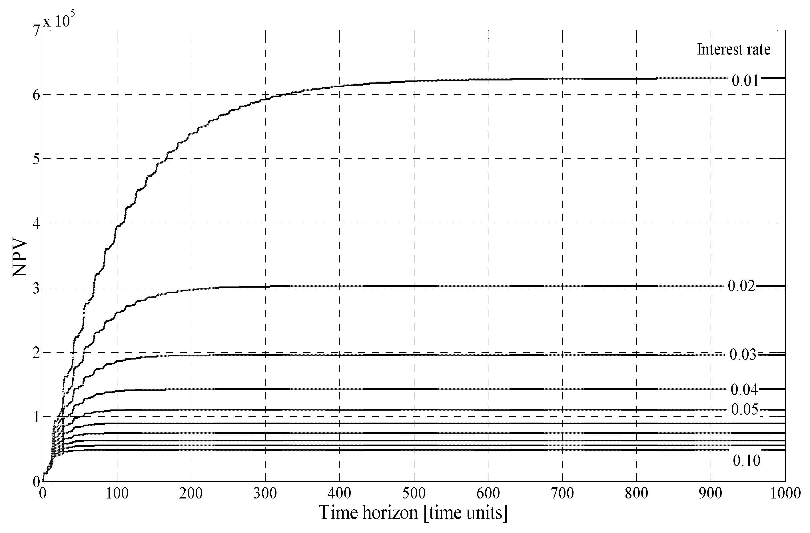
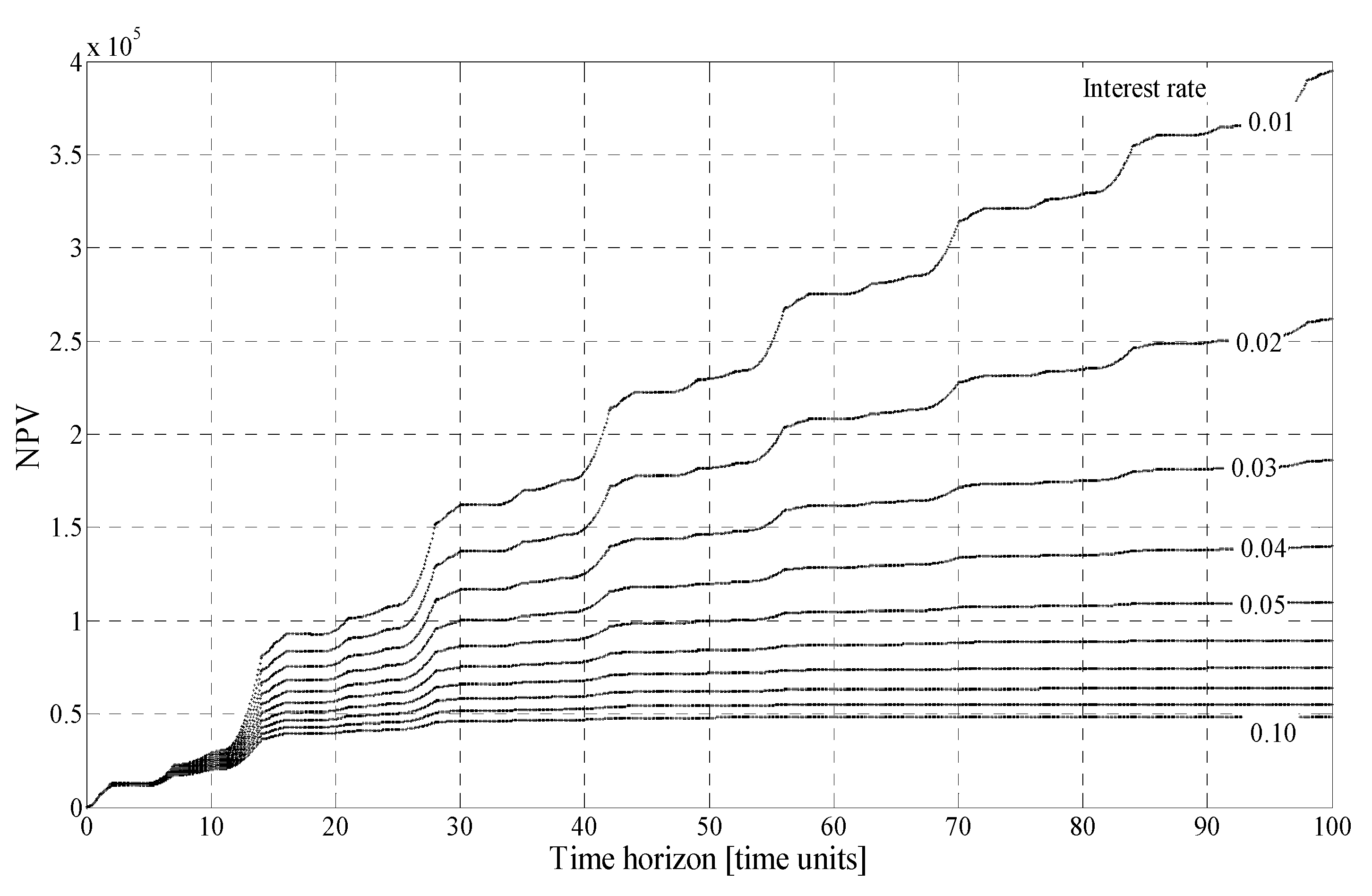
Let us now introduce our novelty, if the time to obsolescence is not known, but would be estimated when considering investments, and that the interest rate could be varying on this time horizon. Using NSM tools, the growth of the NPV to the time to the obsolescence at various interest rates was obtained and is presented in Figure 2, first shown on the time horizon up to 1000. For a shorter time horizon, the details for early obsolescence are given in Figure 3.
The interest rate varies from 0.01 to 0.10 in steps of 0.01. Here, the time delays are not perturbed. The transportation costs are added to the costs of production. Therefore, the NPV on the infinite horizon at different interest rates is very close to the values at the time to obsolescence equal to 1000 time units.
The correction factor for NPV on the finite time horizon was calculated, derived from Table 2. We can see that it is significant at the lower interest rate, but it goes rapidly to 1 when the interest rate is increasing.
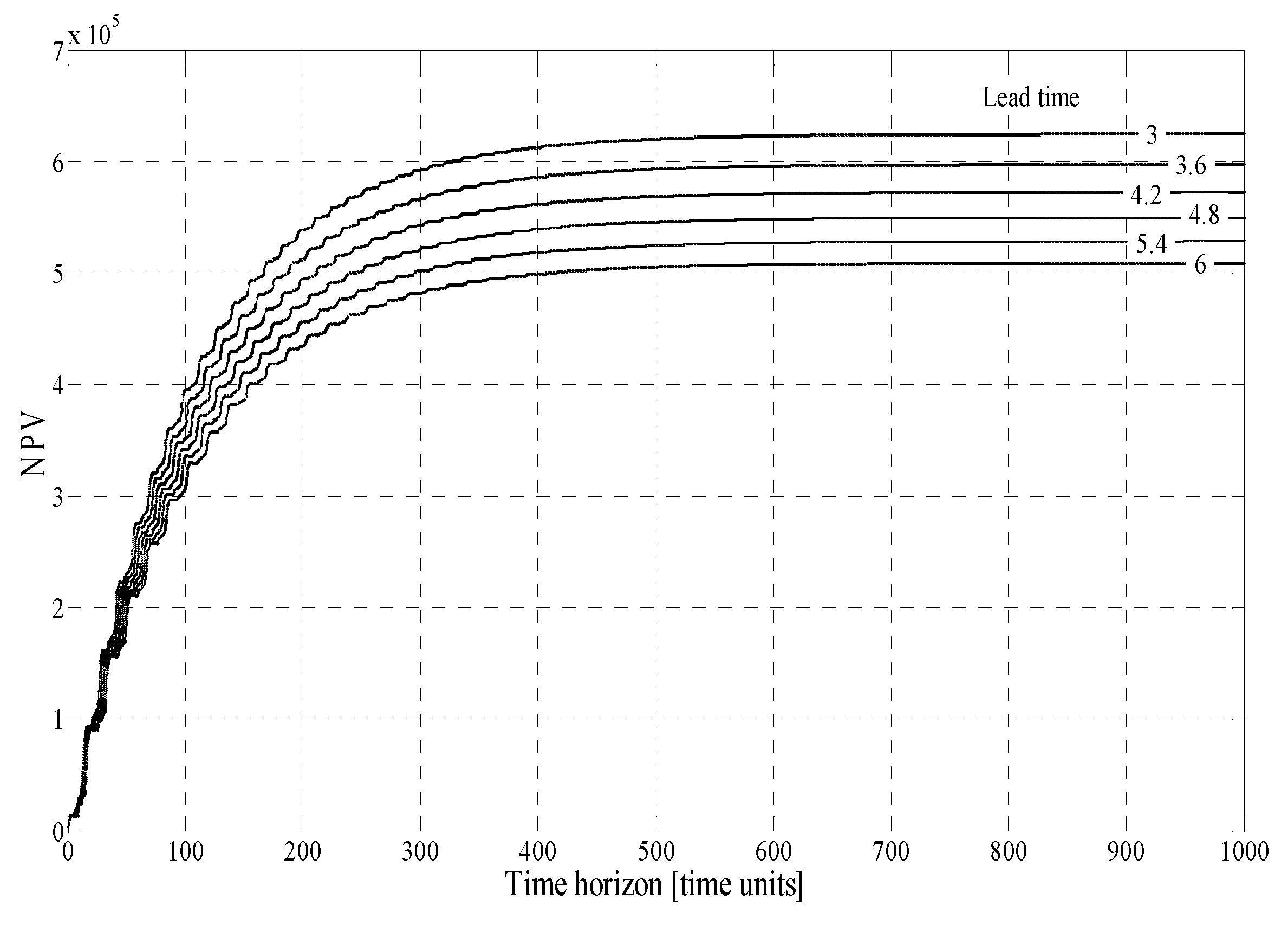
We also analysed the impact of lead time perturbation of different activity cells (production units at various distant locations) on the NPV for the case of obsolescence on the specified time horizon (TTO) given on the abscissa of the figure. Figure 4 shows an example of a variation of NPV when the lead time of D is increasing. Figure 5 shows the details on the shorter time horizon to the obsolescence—a similar approach to statistics that we can use when all activities are delayed simultaneously. From Table 3, we can see that, in the case of a low interest rate, if the time to the obsolescence is only 500 cycles and the interest rate only 1%, then NPV decreases by 1%. If the interest rate is 2% and the time to the obsolescence is only 100 cycles, then NPV reduces by 14%.
We can see in Table 4 that NPV decreases when the lead time is increasing. The relative decrease expressed with the coefficient ϑ was calculated for the perturbation of delays at D and given time to the obsolescence, as presented in Table 5. A similar calculation can also be given for any simultaneous appearance of obsolescence and known distribution of delays.
Using NSM, the behaviour of the NPV can be analysed, when the distribution density functions of lead times or any other time delay, as well as the distribution of the time to obsolescence, is known, and the perturbations appear simultaneously.

5. Discussion

In the case of an SC exposed to the risk of obsolescence in an unknown future, we can judge the time to obsolescence only roughly. The MRP or EMRP evaluation of the NPV under the uncertainty of obsolescence without embedded NSM procedure could be quite highly overestimated, as we can see for our case study in Table 3 and Table 5. For example, if the time to the obsolescence is high enough (1000 time units), then the NPV is well evaluated even if we do not make corrections with the NSM obtained correction factor, as presented in Table 2. Also, at higher interest rates, NSM adjustments are negligible, and the model, presented by Bogataj et al. in [4], is good enough even for the NPV evaluation and evaluation of changes in the NPV at a lower interest rate. However, for a short time to the obsolescence and at a meagre interest rate, which could be cases nowadays, we cannot neglect the correction factor in the NPV estimation. For example, if the interest rate is 2% and obsolescence appears already after 100 time units, NPV in our model is 14% lower than estimated by the extended MRP model, which means that the correction factor λ is 0.86. If the interest rate is 4%, the correction factor is 0.98. Like in the case of our supply chain, for any SC, such estimations can be made and then investments compared with the corrected NPV, like in Table 2, to decide to invest or not in the SC.
On the same way, we can estimate the needed corrections of NPV achieved by the MRP method if the obsolescence appears sooner, but lead times increase. For the case of perturbations in one node (D) of our case study, the correction factors are given in Table 5. If the time to the obsolescence is only 100 time units, and the time delay is equal to 6, the NPV obtained by the MRP model should be corrected by the factor ϑ = 0.777. In case if the time to the obsolescence increases to 1000 time units, however, the correction factor at the same delays is only 0.814. Note also, that while the time to the obsolescence increases to 1000 time units at the delay of 3 time units, NPV obtained by extended MRP method does not need any corrections.

6. Conclusions and Further Research

From the Web of Science Core Collection, there are 71 papers indexed, where the intersection of topics—environment, sustainability, and net present value evaluation of investments—are studied, mainly in journals like Environmental Studies (17), Energy Fuels (11), Engineering Civil (10), Green Sustainable Science Technology (9), and Construction Building Technology (8). The first paper on the intersection of these three topics was published in 2002, but the yearly number of articles is growing rapidly and reached 11 contributions in 2018. Since 2015, in Sustainability, there are 15 papers in which investments have been evaluated using the NPV approach. The articles propose to assess the economic feasibility of environmental protection technology and present the assumptions at which these environment protection systems become economically viable [46]. The profitability analysis is often conducted based on the discounted cash flow method, and the criterion function or a component of it is net present value criterion [8]. In none of these evaluations had the assumption of obsolescence been exposed. As presented in above chapters, however, the obsolescence can significantly reduce NPV and, therefore, the viability of environmental projects.
The uncertainty of viability is increasing by the fast development of the new technologies and increased lead times and their perturbations, owing to the globalisation, which influences obsolescence risks. Obsolescence is only one of the many risks to which supply chains are exposed, but this phenomenon is rarely addressed together with other risks to which production and distribution systems are exposed, as discussed in the work of [47]. The obsolescence risk is the risk that processes in an SC, produced items, total products, or technological solutions in an SC will become obsolete, thus losing the ability to compete on the market. This potential of fast obsolescence reduces the NPV of an SC, and hence the willingness of investors to invest in highly innovative products and banks to give a loan for such investments. In the world of the fast development of technologies, the obsolescence risk is very significant for technology-based SC or their parts when competing in the economy of innovations.
In the article, the need is exposed that this risk should be estimated when members of an SC are deciding how much to invest in new technology. As already mentioned, there is a diverse range of research in financing the supply chain and the impact of the supply chain risks on the financial evaluation of SC. In none of them is the effect of the obsolescence studied systematically. The combination of the MRP method and the NSM can give us a systematic evaluation of risks of obsolescence for any variations of other parameters in the supply chain. In this paper, we have presented the method how to evaluate the perturbations of delays and uncertain value of money (the volatile interest rate) on the finite time horizon concerning total SC through considering the risk drivers and mitigating supply chain risk when one or several parameters are exposed to risk simultaneously and the time to obsolescence is uncertain. The realisation of a supply chain risk influences perturbations in lead times, appearing in transportation routes and nodes of a network, which can be better evaluated in a complex domain for SC operation on the infinite horizon, where they can be summarised and, after this procedure, transformed back to the time domain. In the case in which the time horizon is finite, however, the detailed analysis can be achieved only with a good simulation of the joint perturbations in the SC. Therefore, the simulation tool like that used in our presentation is advised to be embedded in the basic extended MRP model for studying more complex supply chains exposed to the obsolescence.
To include all three main pillars of sustainability in the model, supporting decisions on investments where the impact of innovations in technology are crucial, and the obsolescence is to be expected soon, the presented model should be extended in two directions.
(a)
To study the impact of obsolescence, together with environmental issues, the extension of the presented network is needed, as explained by Bogataj and Grubbström in the article “On the representation of timing for different structures within MRP theory”, where the close loop analysis is given on the infinite horizon [2]. In such cases, some considerations by Kwak and Kim, regarding green profit maximisation through integrated pricing and production planning [48], would also be further studied and evaluated with the NPV criterion, and environmental constraints and penalties.
(b)
Among the social sustainability issues, the main challenges are rising because of the ageing of the European workforce. Therefore, the trade-off between investments in ergonomics and pension schemes for earlier retirement, as presented by Bogataj et al. [49], and other ergonomic improvements should be studied on the finite horizon, which might give different optimal policies for the cases with a smaller ratio between the obsolescence horizon and the value of the length of a cycle. In this case, as well as some other solutions, listed in the articles of Calzavara et al. [50], Battini et al. [51], and Andriolo et al. [52], would be included in the model.

Author Contributions

The initial analysis of the usefulness of the NSM for evaluation of NPV in case of stochastic cash flows on a finite horizon is the result of the joint work of F.C.-B. and J.A.M.-N., while F.M.-G. was also involved in programming the NSM functions. Further studies were developed by all five authors together at facilities of Universidad Politécnica de Cartagena. M.B. and D.B. developed the extension of the MRP model in the way that they were able to evaluate the risks of obsolescence. The final computer program was executed by J.A.M.-N., while D.B. and M.B. wrote this paper.

Funding

This research was partly funded by the Slovenian Research Agency, grant P5-0364 and J6-9396, and partly by the University of Padua.

Conflicts of Interest

The authors declare no conflict of interest.

References

  1. Cabernard, L.; Pfister, S.; Hellweg, S. A new method for analyzing sustainability performance of global supply chains and its application to material resources. Sci. Total Environ. 2019, 684, 164–177. [Google Scholar] [CrossRef] [PubMed]
  2. Bogataj, M.; Grubbström, R.W. On the representation of timing for different structures within MRP theory. Int. J. Prod. Econ. 2012, 140, 749–755. [Google Scholar] [CrossRef] [Green Version]
  3. Bogataj, M.; Grubbström, R.W. Transportation delays in reverse logistics. Int. J. Prod. Econ. 2013, 143, 395–402. [Google Scholar] [CrossRef]
  4. Bogataj, D.; Aver, B.; Bogataj, M. Supply chain risk at simultaneous robust perturbations. Int. J. Prod. Econ. 2016, 181, 68–78. [Google Scholar] [CrossRef]
  5. Despeisse, M.; Baumers, M.; Brown, P.; Charnley, F.; Ford, S.J.; Garmulewiczx, A.; Knowles, S.; Minshall, T.H.W.; Mortara, L.; Reed-Tsochas, F.P.; et al. Unlocking value for a circular economy through 3D printing: A research agenda. Technol. Forecast. Soc. Chang. 2017, 115, 75–84. [Google Scholar] [CrossRef]
  6. Battini, D.; Calzavara, M.; Isolan, I.; Sgaebossa, F.; Zangaro, F. Sustainability in Material Purchasing: A Multi-Objective Economic Order Quantity Model under Carbon Trading. Sustainability 2018, 10, 4438. [Google Scholar] [CrossRef]
  7. Kwak, M. Optimal Line Design of New and Remanufactured Products: A Model for Maximum Profit and Market Share with Environmental Consideration. Sustainability 2018, 10, 4283. [Google Scholar] [CrossRef]
  8. Lin, T.T.; Hsu, S.Y.; Chang, C.C. Evaluation of Decision-Making for the Optimal Value of Sustainable Enterprise Development under Global 100 Index Thinking. Sustainability 2019, 11, 1106. [Google Scholar] [CrossRef]
  9. Alac, P.; Culik, M. Multi-Criteria Decision-Making Model for the Material Flow of Resonant Wood Production. Sustainability 2017, 9, 502. [Google Scholar] [CrossRef]
  10. Harvey, D. The Enigma of Capital and the Crises of Capitalism; Profile Books: London, UK, 2010. [Google Scholar]
  11. Xu, X.; Chen, X.; Jia, F.; Brown, S.; Gong, Y.; Xu, Y. Supply chain finance: A systematic literature review and bibliometric analysis. Int. J. Prod. Econ. 2018, 204, 160–173. [Google Scholar] [CrossRef]
  12. Yan, N.; Sun, B.; Zhang, H.; Liu, C. A partial credit guarantee contract in a capital-constrained supply chain: Financing equilibrium and coordinating strategy. Int. J. Prod. Econ. 2016, 173, 122–133. [Google Scholar] [CrossRef]
  13. Culp, S. Supply Chain Disruption a Major Threat to Business. Forbes 2013. [Google Scholar]
  14. WCED. Our Common Future; Oxford University Press: Oxford, UK, 1987. [Google Scholar]
  15. UN. World Summit Outcome; The United Nations General Assembly; The United Nations: New York, NY, USA, 2005. [Google Scholar]
  16. Faezipour, M.; Ferreira, S. A System Dynamics Approach for Sustainable Water Management in Hospitals. IEEE Syst. J. 2018, 12, 1278–1285. [Google Scholar] [CrossRef]
  17. Eslami, Y.; Dassisti, M.; Lezoche, M.; Panetto, H. A survey on sustainability in manufacturing organisations: Dimensions and future insights. Int. J. Prod. Res. 2019, 57, 5194–5214. [Google Scholar] [CrossRef]
  18. Haanstra, W.; Toxopeus, M.E.; van Gerrevink, M.R. Product life cycle planning for sustainable manufacturing: Translating theory into business opportunities. Procedia CIRP 2017, 61, 46–51. [Google Scholar] [CrossRef]
  19. Dewulf, J.; Mancini, L.; Blengini, G.A.; Sala, S.; Latunussa, C.; Pennington, D. Toward an Overall Analytical Framework forthe Integrated Sustainability Assessment of the Production and Supply of Raw Materials and Primary Energy Carriers. J. Ind. Ecol. 2015, 19, 963–977. [Google Scholar] [CrossRef]
  20. Joung, C.B.; Carrell, J.; Sarkar, P.; Feng, S.C. Categorization of Indicators for Sustainable Manufacturing. Ecol. Indic. 2013, 24, 148–157. [Google Scholar] [CrossRef]
  21. Holton, I.; Glass, J.; Price, A.D.F. Managing for Sustainability: Findings from Four Company Case Studies in the UK Precast Concrete Industry. J. Clean. Prod. 2010, 18, 152–160. [Google Scholar] [CrossRef]
  22. Arena, M.; Duque Ciceri, N.; Terzi, S.; Bengo, I.; Azzone, G.; Garetti, M. A State-of-the-art of Industrial Sustainability: Definitions, Tools and Metrics. Int. J. Prod. Lifecycle Manag. 2009, 4. [Google Scholar] [CrossRef]
  23. Balkema, A.; Preisig, H.; Otterpohl, R.; Lambert, A.J.D. Augmenting Design with Sustainability. Comput. Aided Chem. Eng. 2003, 15, 714–719. [Google Scholar]
  24. Kovačić, D.; Bogataj, M. Net present value evaluation of energy production and consumption in repeated reverse logistics. Technol. Econ. Dev. Econ. 2017, 23, 877–894. [Google Scholar]
  25. Waters, D. Supply Chain Risk Management: Vulnerability and Resilience in Logistics; Kogan Page: Philadelphia, PA, USA, 2007. [Google Scholar]
  26. Yorulmazer, T. Case Studies on Disruptions During the Crisis. In Economic Policy Review; Federal Reserve Bank: New York, NY, USA, 2014; Available online: http://www.newyorkfed.org/research/epr/2014/1402yor1.pdf (accessed on 1 October 2019).
  27. Grubbström, R.W. On the Application of the Laplace Transform to Certain Economic Problems. Manag. Sci. 1967, 13, 558–567. [Google Scholar] [CrossRef]
  28. Grubbström, R.W. Stochastic Properties of a Production-Inventory Process with Planned Production Using Transform Methodology. Int. J. Prod. Econ. 1996, 45, 407–419. [Google Scholar] [CrossRef]
  29. Grubbström, R.W.; Tang, O. An Overview of Input-Output Analysis Applied to Production-Inventory Systems. Econ. Syst. Rev. 2000, 12, 3–25. [Google Scholar] [CrossRef]
  30. Grubbström, R.W. Transform Methodology Applied to Some Inventory Problems. Z. Betr. 2007, 77, 297–324. [Google Scholar] [CrossRef]
  31. Bogataj, D.; Bogataj, M. NPV approach to material requirements planning theory: A 50-year review of these research achievements. Int. J. Prod. Res. 2019, 57, 5137–5153. [Google Scholar] [CrossRef]
  32. Bogataj, L.; Bogataj, M. The study of optimal additional investments in capacities for reduction of delays in the value chain. Int. J. Prod. Econ. 2007, 108, 281–290. [Google Scholar] [CrossRef]
  33. Bogataj, M.; Bogataj, L. Supply chain coordination in spatial games. Int. J. Prod. Econ. 2001, 71, 277–286. [Google Scholar] [CrossRef]
  34. Bogataj, M.; Bogataj, L. On the compact presentation of the lead time perturbations in distribution networks. Int. J. Prod. Econ. 2003, 88, 145–155. [Google Scholar] [CrossRef]
  35. Bogataj, M.; Grubbström, R.W.; Bogataj, L. Efficient location of industrial activity cells in a global supply chain. Int. J. Prod. Econ. 2011, 133, 243–250. [Google Scholar] [CrossRef]
  36. Hudnurkar, M.; Deshpande, S.; Rathod, U.; Jakhar, S.K. Supply Chain Risk Classification Schemes: A Literature Review. Oper. Supply Chain Manag. 2017, 10, 182–199. [Google Scholar] [CrossRef] [Green Version]
  37. Peusner, L. The Principles of Network Thermodynamics: Theory and Biophysical Applications; Entropy Limited: Lincoln, MA, USA, 1987. [Google Scholar]
  38. González-Fernández, C.F. Network simulation method for solving phase-change heat transfer problems with variable thermal properties. Heat Mass Transf. 2002, 38, 327–335. [Google Scholar]
  39. Alhama, F.; Marín, F.; Moreno, J.A. An efficient and reliable model to simulate microscopic mechanical friction in the Frenkel-Kontorova-Tomlinson model. Comput. Phys. Commun. 2011, 182, 2314–2325. [Google Scholar] [CrossRef]
  40. Marín, F.; Alhama, F.; Moreno, J.A. Modelling of stick-slip behaviour with different hypotheses on friction forces. Int. J. Eng. Sci. 2012, 60, 13–24. [Google Scholar] [CrossRef]
  41. Marín, F.; Alhama, F.; Moreno, J.A. Modelling of stick-slip behaviour in a Girling brake using network simulation method. Nonlinear Dyn. 2016, 84, 153–162. [Google Scholar] [CrossRef]
  42. Sanchez-Perez, J.F.; Marín, F.; Morales, J.L.; Canovas, M.; Alhama, F. Modeling and simulation of different and representative engineering problems using Network Simulation Method. PLoS ONE 2018, 13, e0193828. [Google Scholar] [CrossRef]
  43. Basel Committee on Banking Supervision. Guidance on the Application of the Core Principles for Effective Banking Supervision to the Regulation and Supervision of Institutions Relevant to Financial Inclusion; Basel Committee on Banking Supervision: Basel, Switzerland, 2016; Available online: https://www.bis.org/bcbs/publ/d351.pdf (accessed on 1 October 2019).
  44. Hua, Z.; Sun, Y.; Xu, X. Operational causes of bankruptcy propagation in supply chain. Decis. Support. Syst. 2011, 51, 671–681. [Google Scholar] [CrossRef]
  45. Kleindorf, P.R.; Saad, G.H. Managing Disruption Risks in Supply Chains. Prod. Oper. Manag. 2005, 14, 53–68. [Google Scholar] [CrossRef]
  46. Cucchiella, F.; D’Adamo, I.; Gastaldi, M.; Storneli, V. Solar Photovoltaic Panels Combined with Energy Storage in a Residential Building: An Economic Analysis. Sustainability 2018, 10, 3117. [Google Scholar] [CrossRef]
  47. Bogataj, D.; Bogataj, M. Measuring the supply chain risk and vulnerability in frequency space. Int. J. Prod. Econ. 2004, 108, 291–301. [Google Scholar] [CrossRef]
  48. Kwak, M.; Kim, H. Green profit maximization through integrated pricing and production planning for a line of new and remanufactured products. J. Clean. Prod. 2017, 142, 3454–3470. [Google Scholar] [CrossRef] [Green Version]
  49. Bogataj, D.; Battini, D.; Calzavara, M.; Persona, A. The ageing workforce challenge: Investments in collaborative robots or contribution to pension schemes, from the multi-echelon perspective. Int. J. Prod. Econ. 2019, 210, 97–106. [Google Scholar] [CrossRef]
  50. Calzavara, M.; Battini, D.; Bogataj, D.; Sgarbossa, F.; Zennaro, I. Ageing workforce management in manufacturing systems: State of the art and future research agenda. Int. J. Prod. Res. 2019. [Google Scholar] [CrossRef]
  51. Battini, D.; Glock, C.H.; Grosse, E.H.; Persona, A.; Sgarbossa, F. Ergo-lot-sizing: An approach to integrate ergonomic and economic objectives in manual materials handling. Int. J. Prod. Econ. 2017, 185, 230–239. [Google Scholar] [CrossRef]
  52. Andriolo, A.; Battini, D.; Persona, A.; Sgarbossa, F. A new bi-objective approach for including ergonomic principles into EOQ model. Int. J. Prod. Res. 2016, 54, 2610–2627. [Google Scholar] [CrossRef]
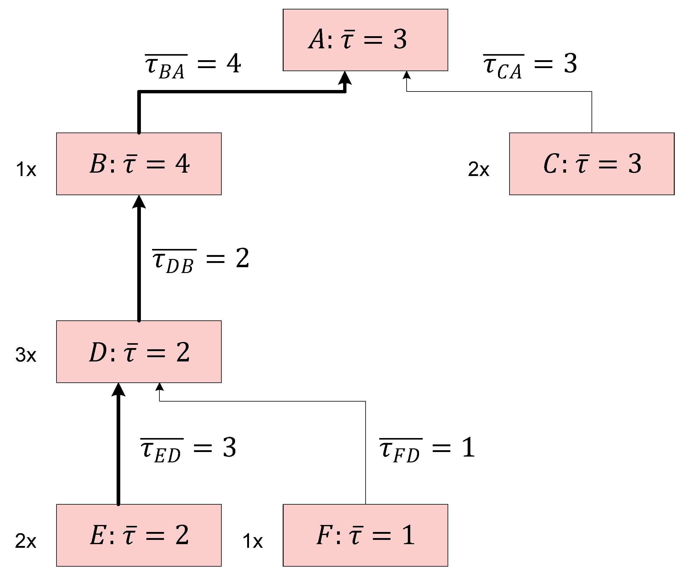
Figure 1. Example of the production in a global supply chain: product structure tree with lead-times shown in the activity cells and on the transportation lines (average lead time τ ¯ . The longest path is denoted by the bold lines).
Sustainability 11 05484 g001
Figure 2. Net present value (NPV) on the time horizon to the time of obsolescence when the interest rate takes a value on the interval [0.01, 0.1].
Sustainability 11 05484 g002
Figure 3. NPV in details on the time horizon lower than 100. The interest rate takes a value on the interval [0.01, 0.1].
Sustainability 11 05484 g003
Figure 4. NPV on the time horizon to the time of obsolescence when the lead time of D is increasing on the interval [3,6].
Sustainability 11 05484 g004
Figure 5. NPV in details when the led time of D is increasing on the interval [3,6].
Sustainability 11 05484 g005
Table 1. The basic notation in extended material requirements planning (EMRP). NPV, net present value.
H; h i , j   HInput matrix (bill-of-materials) describing how many items ( h i , j ) from activity cell i are needed to produce or to package one item in activity cell j
i , j Index of fixed activity cell in a supply chain
G; g i , j GOutput matrix. In our model, we shall assume that G is the identity matrix I
PjPThe intensity of activities in j-th activity cell as a component of production vector P
h i , j   PjThe intensity of flow from i to j
τ j Lead time for the manipulation of the item inside activity cell j
τ i , j Lead time for transportation of items from i to j  
τ Diagonal lead time matrix with element e s τ j in its j -th diagonal position
τ ˜ d ( s ) Perturbed diagonal lead time matrix
s The Laplace (complex) frequency in the Laplace transformed frequency domain
τ j d , τ i j d Additional delays inside the activity cell and transportation line, respectively
H ( s ) ; H ˜ ( s ) ω d Generalised input matrix and the generalised perturbed input matrix
T j Length of the j-th cycle
p , K , Π Price vector, setup cost vector, and transportation cost vector, respectively
F ˜ ( s ) , D, Δ Vector of delivery, the vector of demand and reduction of demand respectively
R(0) R ˜ ( s ) Initial available inventory level and the available interest rate at s
ρ , r Continuous and yearly interest rate, respectively
λThe correction factor for the NPV for various time to obsolescence and various values of the interest rate
ϑThe correction factor for the NPV at different perturbations of lead times and increasing time to the obsolescence
Table 2. NPV in 10,000 € for a different time to obsolescence at a variable interest rate.
Interest RateTime to Obsolescence [Time Units]
[%]1002003004005001000
139.553.859.261.362.062.5
226.229.730.230.330.330.3
318.619.519.619.619.619.6
414.014.214.314.314.314.3
511.011.111.111.111.111.1
68.958.978.978.978.978.97
77.487.497.497.497.497.49
86.386.386.386.386.386.38
95.535.535.535.535.535.53
104.864.864.864.864.864.86
Table 3. Correction factor λ for calculation of NPV for a different time to obsolescence and various values of the interest rate.
InterestTime to Obsolescence [Time Units]
Rate1002003004005001000
0.010.630.860.950.980.991.00
0.020.860.981.001.001.001.00
0.030.950.991.001.001.001.00
0.040.980.991.001.001.001.00
0.050.991.001.001.001.001.00
0.061.001.001.001.001.001.00
0.071.001.001.001.001.001.00
0.081.001.001.001.001.001.00
0.091.001.001.001.001.001.00
0.101.001.001.001.001.001.00
Table 4. NPV in 100,000 € for different perturbed lead times of D and increasing time to the obsolescence.
Lead TimeTime to the Obsolescence TTO [Time Units]
[Time Units]1002003004005001000
3.003.955.385.926.136.206.25
3.603.635.125.675.865.945.98
4.203.524.955.435.625.65.73
4.803.424.715.225.405.465.50
5.403.354.575.025.195.255.29
Table 5. The correction factor ϑ for the NPV at different perturbations of lead times and increasing time to the obsolescence.
Lead TimeTime to the Obsolescence TTO [Time Units]
[Time Units]1002003004005001000
3.001.0001.0001.0001.0001.0001.000
3.600.9190.9520.9580.9560.9580.957
4.200.8910.9200.9170.9170.9180.917
4.800.8660.8750.8820.8810.8810.880
5.400.8480.8490.8480.8470.8470.846
6.000.7770.8090.8140.8140.8150.814