1. Introduction
Understanding urban mobility patterns is important for transportation planning and transportation demand management policy designation. Regular commuting travel demands and irregular leisure travel demands in the subdivisions of a specific geographical area (e.g., traffic analysis zones or grids) can result in different urban mobility patterns [
1]. For example, commuting-related trips represent regular flows between residential areas and business areas, and leisure-based trips that occur in off-work hours are often stochastic movements. Regional-oriented demand strategies may efficiently alleviate traffic congestion. To this end, knowledge of regional-based human mobility patterns could contribute toward establishing planning and management policies.
Currently, urban mobility patterns are generally based on digital footprints, which have benefited from the development of information and communication technology (ICT). Data sources, such as cellular networks [
1], GPS devices [
2], and Wi-Fi hotspots [
3], provide a new opportunity to study the underlying urban mobility patterns. In the existing literature, there are many studies of mobility patterns. Studies can be largely categorized into three groups from the perspective of the research focus: (i) studies of individual mobility mechanisms from a micro-perspective [
4,
5,
6], (ii) studies of aggregate mobility characteristics [
7,
8,
9,
10,
11], and (iii) studies of the interactions between mobility patterns and land use characteristics [
12,
13,
14]. These three categories are not independent. We review some typical works in the remainder of this section.
For the first two categories, mobility patterns are usually studied via metrics derived from individual trips [
15,
16]. Large-scale and high-dimension spatiotemporal datasets are regarded as a reasonable proxy of human mobility. Oliveira showed that human mobility habits are similar regardless of the nature of the dataset, which was based on datasets from eight major world cities [
17]. Many studies have investigated the characteristics of regularity in urban areas. For example, Ma proposed a framework that is capable of identifying the travel patterns of individual transit riders and grouping the corresponding regularity patterns [
18]. Ma focused on transit commuters, identified their travel regularities based on continuous long-term observations, and extracted individual-level residence and workplace data [
19]. Yan and Jiang studied the aggregate mobility patterns by exploring the distance distribution at different spatial scales [
7,
9]. Zhang investigated the statistical properties of taxi trips to characterize travel patterns at seasonal, weekly, and daily time scales [
8]. Yang proposed a method to measure the regularity of travelers and to predict travelers’ future movement between visited locations [
10], whereas Mendoza discovered the regularity mobility patterns for identifying a predictable aggregate ridesharing supply [
11]. Identifying and explaining individual mobility patterns are priorities in studies of collective mobility patterns. However, these studies focus on human-based mobility patterns, and regional mobility patterns and macro-perspective patterns have been less studied.
To contribute to transportation planning over a longer time window, studies have focused on geographical area subdivision-based travel patterns and labeled geographical area subdivisions with distinct characteristics. Clustering algorithms and feature extraction methods are the most popular methods of grouping different geographical area subdivisions. Kang developed a framework to detect spatial taxi operation patterns using matrix factorization, and several typical taxi demand regions and taxi supply regions were investigated [
20]. Demissie applied the fuzzy c-means clustering algorithm to categorize locations with the same features using cellphone data instead of trip data [
21]. The pattern and intensity of urban activities with similar features were detected. However, the detected locations were only a reflection of a subset of the population during a given time window, and the travel tendencies associated with this location were ignored. Alexander clustered locations into groups given the observed duration at each location; these locations were inferred to be a home, workplace, or other location depending on the day of the week and time of day [
22]. Yong used matrix factorization and correlation analysis to extract the stable/occasional components from the collective human mobility data for the Beijing subway [
23]. Although these findings provide insights into the subway’s operations and management, subway networks are biased samples. Call detail records (CDRs) can be regarded as the most complete record of daily mobility, which covers all travel modes. Aniello revealed the demand distribution among different zones and identified the land use through analyzing the outgoing calls for each zone [
24]. Wang revealed hidden patterns in urban road usage for reducing travel time via using CDRs [
25].
Urban activities result in different travel patterns over different time windows, and heterogeneous travel patterns departing from or arriving at different geographical area subdivisions reflect urban land use characteristics. To further explain travel patterns, cellular phone data, GPS data, auto fare collection system (AFC) datasets, and land use characteristic datasets can be combined to assess the relations among land use and travel patterns. Notably, land use characteristics affect physical activity [
26]. Thus, detailed insight into spatiotemporal travel patterns can be obtained by considering a land use dataset [
27,
28]. The relationships between land use characteristics and bus rapid transit (BRT) station demands were examined in [
28], and the results suggested that the extent of developable land around a station determines the BRT traffic flow. After mining passenger routes among all metro stations and exploring the spatial heterogeneity of the dynamic space, Gong found that check in/out passenger flows are highly related to the land use structure around metro stations [
13]. Gan studied the relationship between mobility patterns and land use in the Nanjing metro, and metro stations were classified into classes with different travel characteristics [
29]. The relations between land use characteristics and mobility patterns can be investigated using correlation analysis. Correlation analysis can identify the mobility patterns at a given location specifically due to the existing land use characteristics. Thus, the influence of land use characteristics on mobility patterns should be further discussed at a large geographical scale.
In summary, most studies have focused on investigating mobility patterns. Groups of individuals with different mobility patterns and their corresponding impact factors have been extensively studied. However, there is still room for improvement in research on this topic.
- i
Regional-based mobility patterns, which can provide macro-insights into mobility patterns, have not been fully analyzed.
- ii
The influence of regional land use on mobility patterns has not been studied from a quantitative perspective.
To achieve these improvements, we develop and implement a multistep method using mobile phone data and point-of-interest (POI) data to analyze traffic analysis zone (TAZ)-based mobility patterns and explore the relations between land use characteristics and mobility patterns. The contributions of this work are as follows.
We categorize the TAZs with similar daily TAZ-based mobility patterns into different groups. The travel intensity and differences in departure and arrival are used to separate each group.
We investigate the relations between land use characteristics and mobility patterns. The occurrence probability of different mobility patterns with respect to the relevant land use characteristics is explored from a quantitative perspective.
We apply our workflow to a real-world dataset in a selected metropolitan area of Beijing, China.
The remainder of the paper is organized as follows. The next section presents the methodology, followed by empirical analysis. Finally, we conclude the paper.
2. Methodology
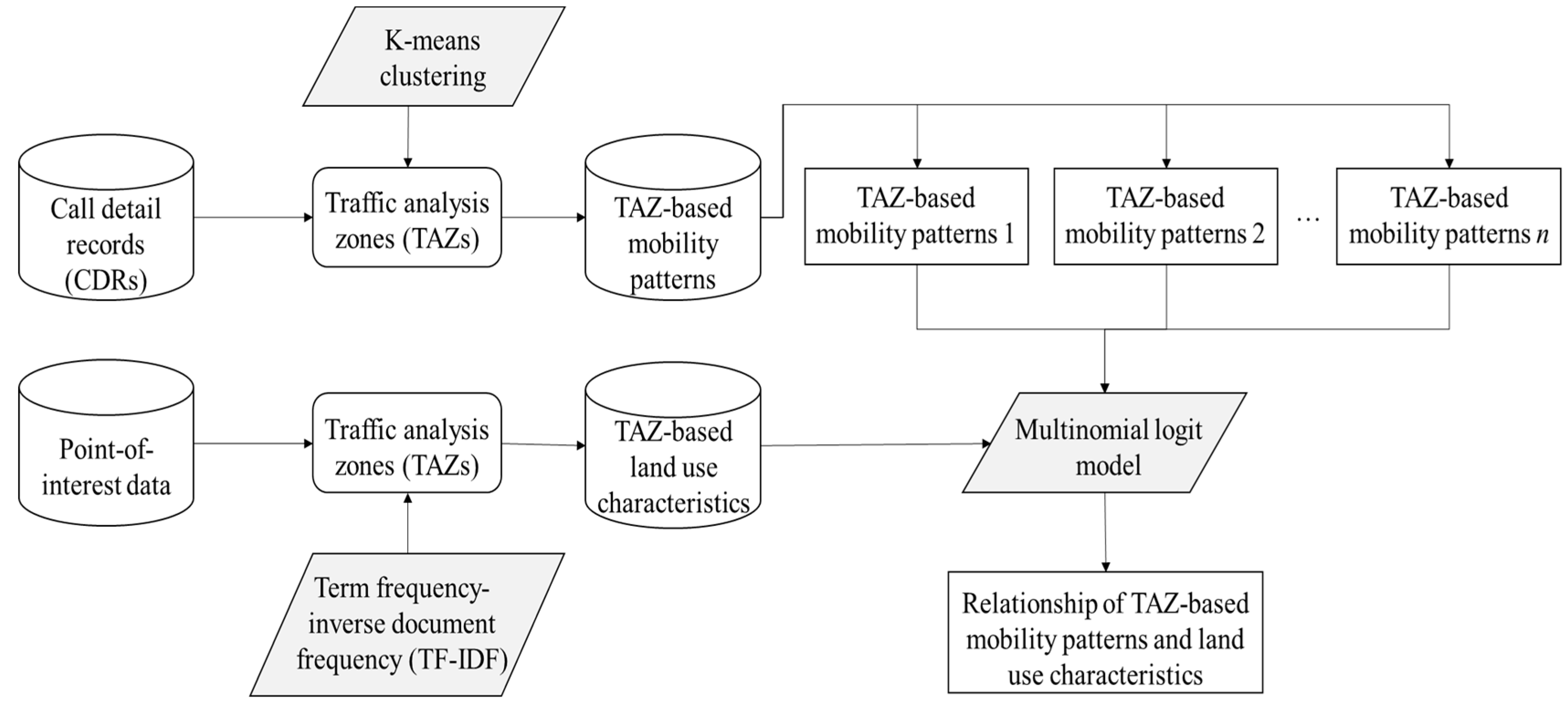
To assess the relationship of TAZ-based mobility patterns and land use characteristics, TAZ-based mobility patterns identification and land use characteristics representation are the preliminary methods. A clustering method is an efficient method to distinguish TAZ-based mobility patterns while considering hourly generation and attraction mobility trips in each TAZ. We first used cluster analysis to categorize TAZs into different groups based on arrival and departure mobility patterns with similar temporal profiles. Then, we needed to find a good representation of a TAZ’s land use characteristics due to the urban planning map not being publicly available. Based on this, we introduced a method to characterize the land use type within TAZs using POI data. As for the relationship of discretized TAZ-based mobility patterns and land use characteristics corresponding to each TAZ-based mobility pattern group, multinomial logit regression could interpret its interactions. Finally, we investigated the possibility of creating different mobility pattern groups with respect to different land use characteristics using a multinomial logit model. The workflow of this study is shown in
Figure 1.
2.1. Cluster Analysis
In general, popular approaches to defining the variables in a time series cluster analysis consist of using the statistical characteristics of mobility patterns or directly using the mobility patterns. The first type of approach extracts key features from mobility patterns as candidate variables. The latter is a straightforward method of representing the daily mobility patterns of a TAZ.
Let denote a mobility pattern observation for TAZ i, where n represents the dimension of the attributes being clustered and d = 1, …, n denotes the indices of the attributes. Specifically, may indicate the departure/arrival trips in time window d. We use to represent all the mobility patterns, with I = 1, …, m denoting the TAZ index.
Mobility patterns vary by TAZ over the course of the day, and the mobility patterns in all time windows can be combined to obtain the overall mobility pattern information. Because hourly mobility patterns are corresponding to each TAZ, hourly departure and arrival trips can be used as variables. Here, we use the number of hourly arrival and departure trips as candidate variables in cluster analysis. To this effect, each TAZ has 48 (departure/arrival trips × 24-h time windows) variables for the cluster analysis. It is necessary to perform normalization to account for the different land use characteristics among TAZs. The normalization equation is expressed as follows:
where
is the
-th hourly number of trips being normalized in TAZ
is the arithmetic mean of the hourly number of trips in TAZ
, and
is the standard deviation of the hourly number of trips in TAZ
.
Among all clustering methods, K-means clustering is generally considered one of the most basic clustering algorithms based on the centroid model [
30]. One weakness of the K-means method is the number of clusters that need to be predetermined. As a result, an objective criterion is required to assess clustering performance because the optimal value of K is often difficult to constrain. Therefore, we applied the Davies and Bouldin [
31] index and Silhouette [
32] index to determine the optimal cluster number K. Then, we applied the K-means algorithm to partition the observations into K clusters.
2.2. Constructing Land Use Vectors Using POI Data
To assess the relations between mobility patterns and land use characteristics, a land use characteristic dataset is needed. In general, the POI dataset collected by the Google Place API [
33] has been used to represent land use characteristics.
A POI consists of a category, name, and location (latitude and longitude). For each TAZ, we can learn the land use structure in a TAZ by computing the term frequency-inverse document frequency (TF-IDF) using POIs [
34]. Specifically, this variable is calculated as follows.
For a given TAZ
,
a POI vector,
, can be obtained, where
(
j = 1, …,
C) is the TF-IDF value of the
j-th POI category and
C is the number of POI categories. The TF-IDF value
is given as follows:
The TF term is on the left-hand side of Equation (2), where represents the number of POIs belonging to the j-th category and represents the number of POIs in TAZ . The IDF term is the total number of TAZs m divided by the number of TAZs that include the j-th POI category. Then, the logarithm of that result is calculated. indicates the number of TAZs that include the j-th POI category.
2.3. Multinomial Logit Model
Land use characteristics are coupled with human travel patterns [
26]. To this end, the regional mobility patterns can be changed when the land use characteristics are changed in the long time window. Note that the change of land use characteristics results from the urban long-term dynamic mechanism, which involves many factors, such as policy, population changes, traffic network, and so forth. Building a model that explains this complex mechanism requires more data and more comprehensive knowledge, which was not available to this study. Therefore, we attempted to establish the relations between traffic analysis zone-based mobility patterns and land use characteristics rather than discussing urban long-term dynamic mechanisms.
In this study, we defined the relations as the probability of different mobility patterns being associated with different land use types. The relations could be captured by a discrete choice model, such as a logit or multinomial logit model. As discretized TAZ-based mobility patterns in urban areas may be more than two categories, a multinomial logit model can generalize logit regression for multivariable problems. Specifically, it is a model that is used to predict the probabilities of the different possible outcomes of a categorically distributed dependent variable, given a set of independent variables. A multinomial logit model with
j dependent variables is:
where
is utility functions of a multinomial logit model and
is the vector of independent variables. The utility function indicates the utility extent of independent variables
being causally linked to a
j-th dependent variable, and it can be formulated as:
where
is the coefficient, and
is an error term subjected to the Gumbel distribution. Parameters can be estimated using the maximum likelihood. The fitness of the model can be evaluated using pseudo-
R2, which is as follows:
In general,
R2 ranges from 0 to 1. A higher
R2 indicates a good fitness of the model, and vice versa. Mcfadden found that a model has a good interpretation and prediction performance when
R2 is bigger than 0.2 [
35].
This model can predict the probabilities of the different possible outcomes of a categorically distributed dependent variable given a set of independent variables. The results can show how mobility patterns and land use are causally linked. Here, clusters of TAZs with different mobility patterns are categorically distributed dependent variables, and land use characteristics are a set of independent variables. By combining the cluster results and POI vectors in TAZs, a multinomial logit model was established to investigate the relations between land use and TAZ-based mobility patterns. The probability of a TAZ being categorized into a given cluster is described as follows:
where
indicates TAZ
i being categorized into cluster
j, and
J is the number of categorized TAZ-based mobility patterns. In this approach, the relationship between mobility patterns and land use characteristics can be reflected by this coefficient. Moreover, a multinomial logit model is a nonlinear model, and the coefficient could not represent the marginal utility of each land use characteristic for TAZ-based mobility patterns. In fact, the marginal utility of the independent variable is the partial derivative of the probability of categorized TAZ-based mobility patterns. For the marginal influence of a certain independent variable, its value is when other variables remain unchanged and the independent variable changes 1 unit for the TAZ-based mobility patterns.
3. Case Study
3.1. Study Area and Data Description
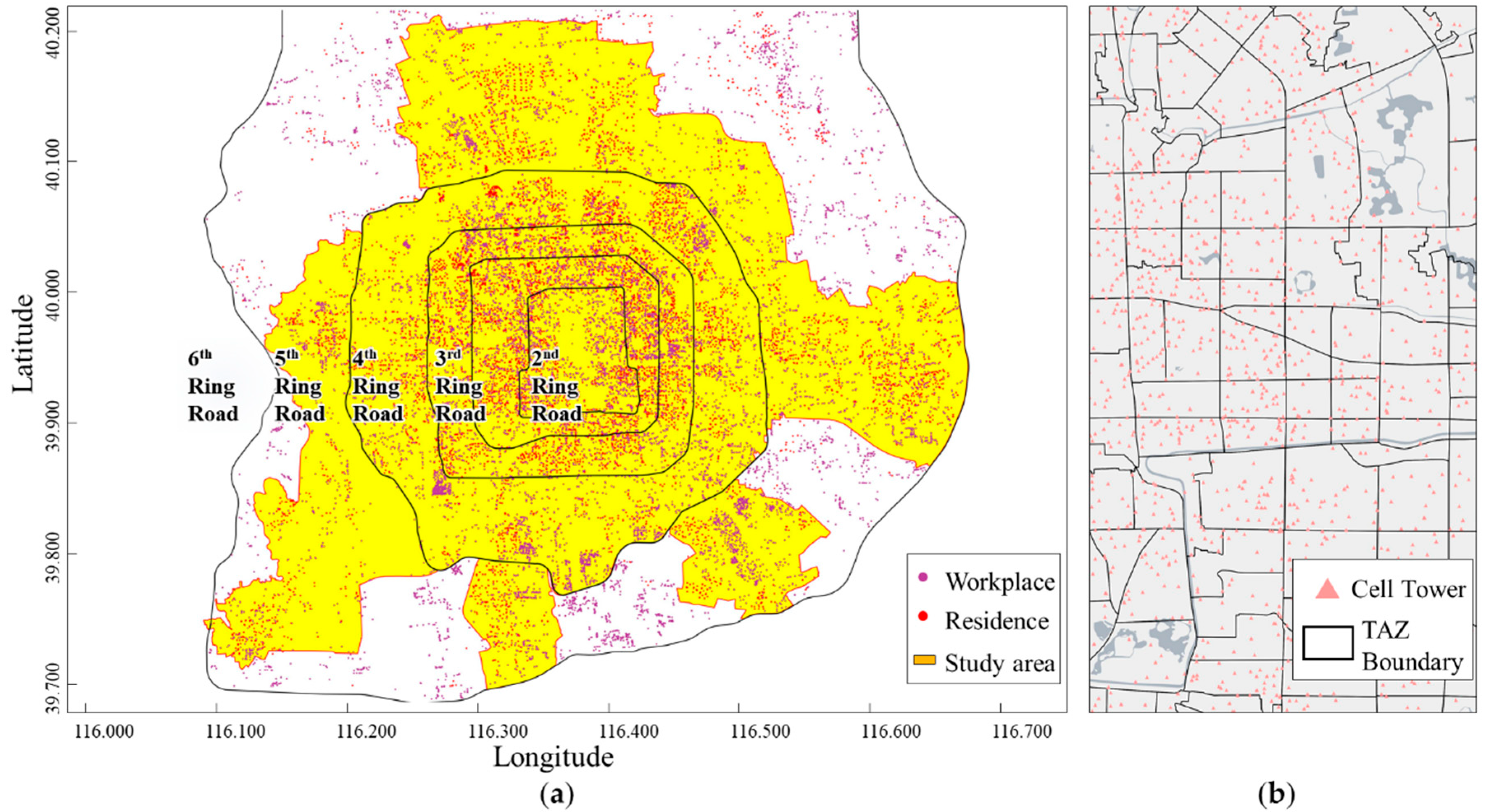
Beijing covers a total area of 16,410.54 square kilometers. Six ring roads segment urban areas into several subdivisions with unbalanced job and housing distributions. Inhabitants within the Sixth Ring Road account for 78% of the total permanent population in the city, and 43% of this population is within the Fifth Ring Road. Inhabitants between the Fifth Ring Road and Sixth Ring Road are centrally distributed around several large residential communities. Additionally, 80% of workplaces are located within the Sixth Ring Road, and 51% are within the Fifth Ring Road. Few workplaces are available between the Fifth and Sixth Ring Roads [
36]. In this context, urban areas within the Fifth Ring Road and some large residential communities between the Fifth Ring Road and the Sixth Ring Road were selected as the study area.
Figure 2a shows the spatial residence and workplace distributions within the Sixth Ring Road from the POI dataset.
We investigated the relationship between TAZ-based mobility patterns and land use characteristics based on large-scale, high-penetration mobile phone data and POI data. Data descriptions are given below, and the preparation of each dataset is described.
Beijing has a high number of mobile phone users. By the end of 2018, the average number of mobile phones owned per 100 persons among inhabitants was 172.9 [
37]. Here, we first used anonymized mobile phone CDRs from Beijing for the period from 1 June to 7 June 2015 as our original trajectory dataset. The data were collected by one large mobile operator in Beijing whose subscribers account for 67% of all mobile phone users. CDRs are made up of millions of records that are triggered by events such as calls and short messaging services (SMS), or by regular updates of the network. Each record has an anonymized user ID, cell location, and timestamp.
TAZ is a spatial unit of planning area used for Beijing transportation planning purposes by the Beijing transportation institute. There are 1127 TAZs in the study area with sizes ranging from 0.13 square kilometers to 10.31 square kilometers.
Figure 2b exhibit the relationship between TAZs and cell towers. As the number of cell towers in a TAZ depends on the land use type and population within a TAZ, the TAZ boundary is used for dividing the cell towers into different TAZs. We analyzed the phone users at the tower level to estimate generation/attraction at the TAZ level.
In this study, we only focused on the mobility patterns on weekdays, and we adopted 18 million anonymous user records from 1 June to 5 June 2015 to extract traveler trip information. The mobile phone data were cleaned and processed as follows.
- Step 1:
We removed records in which the user ID, timestamp, or coordinates were missing.
- Step 2:
Of the selected data records, 18,096,128 unique user IDs were identified. We only used the data from users with more than one base station location recorded. Then, we ranked the records by user ID and timestamp in ascending order.
- Step 3:
Using the records, we could extract trips from mobile phone data by following a commonly used method [
21]. Given that we focused on human mobility pattern profiles within TAZs, if a user was recorded at a mobile phone base station, we simply mapped the user to the TAZ where the base station was located.
- Step 4:
One day was split into 24-time windows. For each hourly time window t, we pinpointed the origin and destination TAZ in which each mobile phone user was located. Then, we aggregated the movements with the same origin and destination TAZs into time window t.
- Step 5:
Inter-TAZ trips were extracted, and trips with the same origin and destination were not considered. In this step, the hourly numbers of arrival and departure trips in each TAZ were determined. The number of trips was scaled by the mobile operator market share (m = 1/0.67 1.5).
3.2. Results of the Cluster Analysis
In this section, we first examined the results of tests for K = 2 to K = 10 derived from the average Silhouette index and Davies–Bouldin index, where the optimal number should be 4 according to the Silhouette index and Davies–Bouldin index. Consequently, 1127 TAZs were categorized into four groups. Then, we built the temporal mobility patterns and spatial distribution profiles of each group of TAZs in
Figure 3 and
Figure 4. The four groups of mobility patterns exhibited different characteristics.
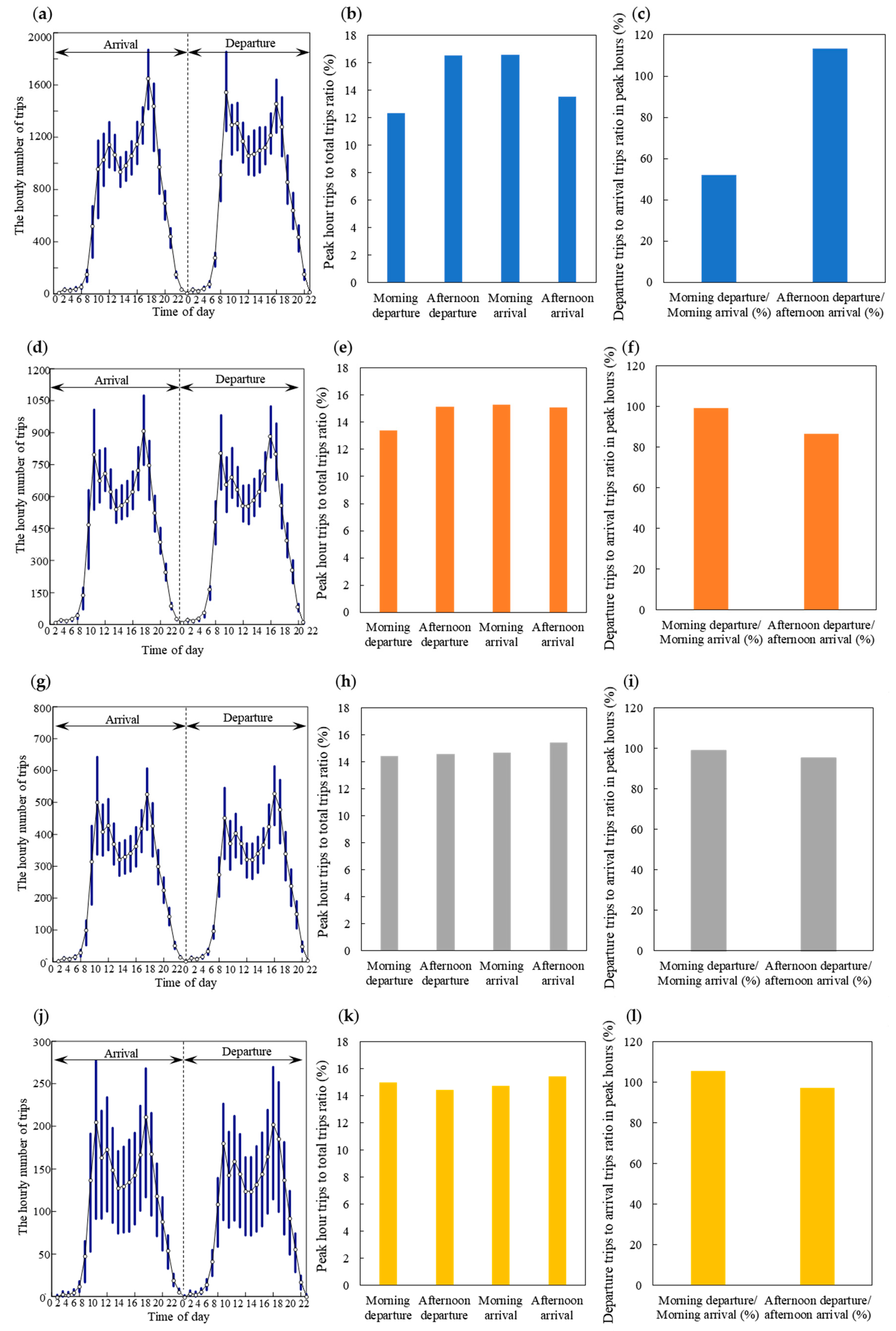
From a temporal perspective,
Figure 3 shows a clear difference in the total amount of travel intensity for each group, and the average travel intensity of TAZs decreased in the order of clusters 1 to 4. Here, travel intensity depicted the total number of hourly departure and arrival trips in a TAZ. Additionally, the variations in mobility patterns during each time window were investigated by presenting the first and third quartiles of the total trips in each panel of
Figure 3. Finally, we defined each group of TAZs based on the corresponding travel intensity as follows:
significant travel intensity TAZs (cluster 1, including 78 TAZs);
normal travel intensity TAZs (cluster 2, including 249 TAZs);
moderate travel intensity TAZs (cluster 3, including 362 TAZs); and
low travel intensity TAZs (cluster 4, including 438 TAZs).
Cluster 1: For both arrival and departure trips in cluster 1, the highest hourly number of trips could reach 2000.
Figure 3a shows that the changes in the number of hourly trips in this cluster were higher than those in other clusters. Thus, the travel intensity of cluster 1 was high, but this value was less distinguishable among other clusters. Additionally, the ratios of departure trips to arrival trips and hourly trips to the total number of trips were the highest among all clusters (
Figure 3b,c). This result suggested that these types of TAZs were attraction-oriented during the morning peak hours and generation-oriented in the afternoon peak hours. In reality, the temporal distribution of trips was unbalanced, and the peak-hour characteristics were prominent in these TAZs compared to those in other types of TAZs. This cluster represented the temporal profile of workplace-oriented TAZs.
Cluster 2: For both the arrival and departure trips in cluster 2, the highest number of hourly trips for normal travel intensity TAZs was less than 1200. The temporal profiles of departure trips and arrival trips exhibited similar peaks, and there was a slight difference between the number of trips in peak hours and the total number of daily trips (
Figure 3d,e). As shown in
Figure 3f, these TAZs shared some common characteristics: the generation and attraction travel intensities were nearly balanced, with a ratio above 85%. Slight differences, however, were observed from departure trips to arrival trips, and this finding was similar to that for cluster 1, but vastly different than the results for the other two groups. With the temporal mobility profiles and travel intensities, we could determine that this cluster reflected the travel activities and patterns in residential areas. Because commuters often made sequentially planned movements for various purposes in the afternoon peak hours [
1], it was unlikely that there would be a significant difference between the average number of departures and arrivals. These TAZs were usually located in urban residential communities or the community outside the Fifth Ring Road, where job housing was relatively abundant. Overall, this cluster mainly included residence-oriented TAZs.
Cluster 3: In this cluster, TAZs with a maximum of 800 average hourly trips were classified as having a moderate travel intensity. For arrival trips, a large variance was observed during morning peak hours, but this variance was still lower than those for cluster 1 and cluster 2 (
Figure 3g). The ratio of the number of trips during peak hours to the total amount of daily trips displayed few differences (
Figure 3h), indicating a balance between departure trips and arrival trips in the same time window. Moreover, the generation and attraction difference between the morning peak and afternoon peak was the smallest among the four groups, as shown in
Figure 3i. As indicated by
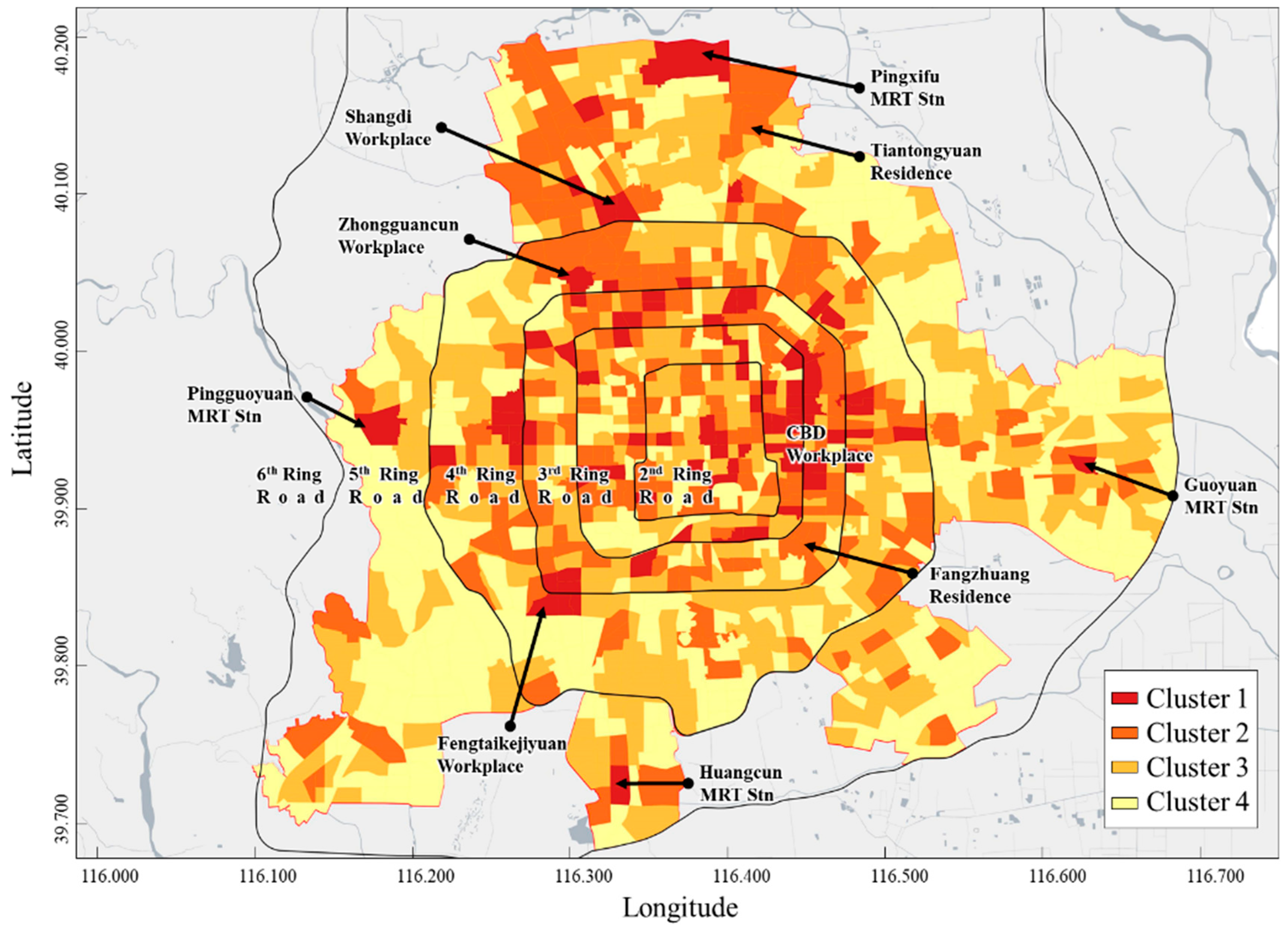
Figure 4, the clusters in this group were mainly located in the areas neighboring residential communities and workplaces. Thus, these TAZs had low population densities and travel intensities, and most trips passed through these areas rather than originating or departing from them. Consequently, the intensity level was moderate for these TAZs.
Cluster 4: The remaining TAZs, with no more than 300 departure and arrival trips on average, were associated with a low travel intensity pattern that varied greatly during a given time window. As shown in
Figure 4, these types of TAZs were located in less-developed urban areas and at the margins of residential communities and some green land use areas. Thus, these TAZs corresponded to few human movements, usually including stochastic trips. Given that the travel intensity of this cluster was markedly lower than those of other clusters, the average hourly numbers of arrival and departure trips accounted for a significant proportion of the total number of daily trips (
Figure 3k). Moreover, the numbers of arrival trips and departure trips during peak hours were nearly the same (
Figure 3l). There was no significant population entering or exiting these TAZs during a given time window, and population changes were relatively stable over the course of a day.
By fixing the peak hours of the day, we determined the ratio of peak-hour trips to the total number of daily trips and the ratio of departure trips to arrival trips, as seen in
Figure 3. Note that the TAZs in cluster 1 tended to have high differences (
Figure 3b,c), indicating that departure trips and arrival trips were imbalanced, particularly during peak hours. Additionally, departure and arrival trips in TAZs with low travel intensities, such as clusters 3 and 4, tended to be relatively balanced.
From a spatial perspective, as shown in
Figure 4, travel activities were concentrated in particular areas of Beijing. The spatial distributions were concentrated within the east Third Ring Road and east Fourth Ring Road, and TAZs with significant travel intensities were observed outside the Fifth Ring Road. For example, there was a higher travel demand within the north Fifth Ring Road than within the Sixth Ring Road because it included a large residential community.
3.3. Relationship between TAZ-Based Mobility Patterns and Land Use Characteristics
Previous studies have been conducted to assess the relationship between traveling activities and land use characteristics [
38]. These studies, which focused on the statistical correlations, identified a close relationship between land use and mobility patterns. This section examines the co-occurrence probabilities among different TAZ-based mobility patterns and land use characteristics derived from POI data.
As TAZ-based mobility patterns are specific to different locations with different urban functions, POI data and clustered TAZs, in combination, can reveal important information about mobility patterns.
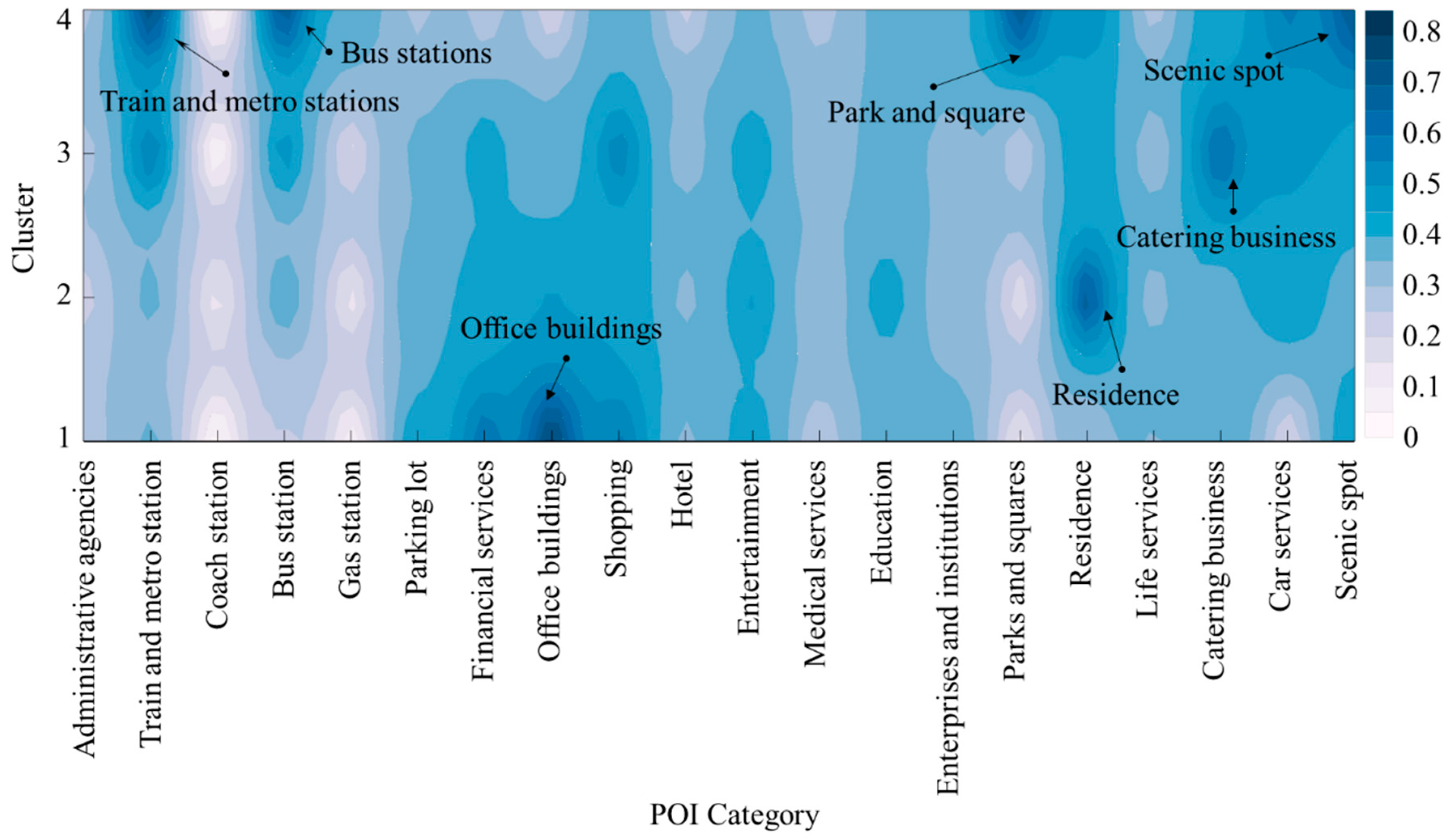
Figure 5 displays the distribution of land use characteristics through the averaged land use vector obtained using Equation (2). Note that there were seven dense points in the heat map, and labels were given beside the dense points.
For land use vectors in all TAZs, cluster 1 was dominated by the workplace land use type, and the residence land use type was dominant in cluster 2. Cluster 3 was characterized by commercial and entertainment land use types, such as life services and catering businesses, which were associated with moderate travel intensities. Cluster 4, however, had the highest proportions of train and metro stations, bus stations, parks and squares, and scenic spots, indicating that TAZs in Cluster 4 tended to be characterized by the public facility land use type.
Overall, the trips extracted from mobile phone data identified the entire travel process. Because “last-mile” and “first-mile” strategies are prevalent in large cities, bus stations and metro stations are usually the transfer point during a trip. Thus, in addition to the green land use type, urban infrastructure-like transportation facilities could fall into Cluster 4.
In general, workplaces, residences, green land use areas, and public facilities, such as bus stations, accounted for a significant proportion of all land use indicators. Other elements in the POI vector were not obvious, and we merged POI categories together to increase the observed counts. After merging the POI points into administrative area, commercial and business area, residence, transportation facility, and green area and square categories, a multinomial logit model was used to investigate the relations between TAZ-based mobility patterns and land use indicators. The results are shown in
Table 1.
The model took cluster 4 as a reference dataset. As described previously, cluster 4 included a group of TAZs with low travel intensities and no obvious differences in departure and arrival trips during peak hours. Other clusters were used to investigate the reasonability of assigning selected clusters to reference datasets. The coefficient reflected the risk probability of assigning a TAZ with specific land use characteristics to the reference cluster. The coefficient of these clusters could thus be used to represent the occurrence probabilities of different mobility patterns with respect to the relevant land use characteristics.
For a given cluster, a positive coefficient indicated low similarity with cluster 4, and vice versa. This result verified that clear relations existed among land use characteristics and TAZ-based mobility patterns. As expected, the administrative area and commercial and business area categories largely influenced TAZ-based mobility patterns, such as those in cluster 1. It was likely that travelers would arrive at these locations from 7:00–9:00; then, travelers would start their trip home between 17:00 and 19:00. Although the risk of unreasonably grouping residences and transportation facilities may increase, these categories had little effect on the results because of the small coefficient. As shown in
Figure 4, the Shangdi, Zhongguancun, central business district (CBD), and Fengtaikejiyuan TAZs were categorized into cluster 1, which was characterized by typical workplace land use types. Additionally, some transfer metro stations, such as Pingguoyuan Metro (MRT) Station, Pingxifu MRT Station, and Guoyuan MRT Station, shared the characteristics of TAZs in cluster 1.
For cluster 2, the positive coefficient for residences reflected the average travel intensity of the corresponding TAZs and the observed departure-oriented phenomenon in the morning peak hours. A large proportion of the residence land use type in a TAZ would increase the possibility of grouping this TAZ into cluster 2. However, the negative coefficient in cluster 2 indicated a low probability of having administrative areas and commercial and business areas in cluster 2. This coefficient was generally positive for locations that included residence communities, such as Tiantongyuan and Fangzhuang (
Figure 4).
For TAZs in cluster 3, the inclusion of transportation facilities and green land use types influenced the distinct temporal profile of cluster 3. As indicated by
Figure 4, cluster 3 had a moderate travel intensity due to the marginal locations of the TAZs in the cluster in residential and workplace areas. As a result, the locations of transportation facilities had a significant impact on the temporal mobility patterns of cluster 3. In addition to workplaces and residences, the TAZs within the Fourth Ring Road were generally categorized into cluster 3 and were more scattered than those outside the Fourth Ring Road (
Figure 4).
4. Discussion
For the TAZ-based mobility patterns, there were four types of TAZs with different travel intensities. We defined these groups as high travel intensity TAZs, normal travel intensity TAZs, moderate travel intensity TAZs, and low travel intensity TAZs. The categorized TAZs and land use indicators derived from POI data were combined to reveal the important semantic information associated with each group. The details are given as follows.
Cluster 1 had a high travel intensity and a notable difference in the numbers of hourly arrival trips and departure trips during peak hours. This finding suggests that TAZs in this group were arrival-oriented in the morning and departure-oriented in the afternoon.
The TAZs in cluster 2 had a departure tendency (versus arrivals) in the morning and an arrival tendency (versus departures) in the afternoon. Therefore, these TAZs mostly included residence-oriented land use types.
The TAZs with moderate travel intensities were assigned to cluster 3. Significant differences in the numbers of departure and arrival trips did not exist because this group of TAZs was mainly located in neighboring residential communities and workplaces.
The remainder of the TAZs with the smallest travel intensity belonged to Cluster 4, and most of them were located in less-developed urban areas and green land use areas.
Regarding the relations between TAZ-based mobility patterns and land use indicators, the results of the multinomial logit model indicated that land use indicators, such as residence and commercial and business area indicators, were correlated with specific temporal TAZ-based mobility patterns. Notably, the results suggested that an imbalanced land use distribution could produce significant differences between arrival trips and departure trips during peak hours. A high proportion of workplace land use types would likely result in temporal TAZ-based mobility patterns similar to those of cluster 1. Likewise, a dominance of residences in a TAZ could lead to temporal TAZ-based mobility patterns similar to those of cluster 2. These TAZ categorization results could be used to design TAZ-based demand management strategies.
5. Conclusions
The development of ICT has allowed the human “digital footprint” to be widely used in transportation systems. This ability has resulted in new opportunities, but also major challenges, for transportation planners. The consideration of this information can affect how transportation systems and demand management policies are designed and implemented. Many studies have focused on analyzing human mobility patterns. Limited research efforts have been devoted to revealing TAZ-based mobility patterns. In this study, we analyzed a mobile phone dataset and a POI dataset. Based on millions of trips extracted from mobile phone data, we built TAZ-based temporal mobility pattern profiles and categorized urban areas into four groups. A multinomial logit model was then used to investigate the relations between TAZ-based mobility patterns and local land use characteristics. The following findings were obtained. From a methodological perspective, we built a multistep methodology to reveal the TAZ-based mobility patterns and study the occurrence probability of different mobility patterns with respect to the relevant land use characteristics. To determine the TAZ-based mobility patterns, an unsupervised clustering algorithm was applied to categorize TAZs with different temporal mobility profiles into several groups. Additionally, a multinomial logit model was developed to calculate the occurrence probability of different mobility patterns with respect to the different land use characteristics. From the perspective of our case study, previous studies that focused on individual or collective mobility patterns provided insights into the human mobility patterns in Beijing. Here, we focused on identifying the temporal mobility patterns in TAZs and determining what types of land use characteristics shaped mobility patterns. Through the interpretation of our findings, we recognize the necessity for further work. First, future studies should investigate the TAZ-based mobility patterns over different time periods, such as weekdays, weekends, and seasons. Second, more cross-validation studies need to be done. We acknowledge that the origin and destination identification method using mobile phone data is not sensitive to short trips. As a result, more cross-validation analyses combining data, such as AFC and GPS datasets, are needed. Finally, comparative and empirical studies across cities can enrich the TAZ-base mobility patterns in the future.


