Mixed Layer Heat Variations in the South China Sea Observed by Argo Float and Reanalysis Data during 2012–2015

Abstract

The atmospheric and oceanic causes of mixed layer heat variations in the South China Sea (SCS) are examined using data from six long-lived Array for Real-time Geostrophic Oceanography (Argo) floats. The mixed layer heat budget along each float trajectory is evaluated based on direct measurements, satellite and reanalysis datasets. Our results suggest that the mixed layer heat balance in the SCS has distinct spatial and seasonal variations. The amplitude of all terms in the mixed layer heat budget equation is significantly larger in the northern SCS than in the southern SCS, especially in winter. In the northern SCS, the mixed layer heat budget is controlled by the local surface heat flux and horizontal advection terms in winter, and the net heat flux term in summer. In the western and southeastern SCS, the mixed layer heat budget is dominated by the net surface heat flux in both winter and summer. Further analysis shows that in the SCS, surface shortwave radiation and geostrophic heat advection are major contributors to net heat flux and horizontal advection, respectively. Unlike the net heat flux and horizontal advection, the vertical entrainment is a sink term in general. The rate of mixed layer deepening is the most important factor in the entrainment rate, and a barrier layer may decrease the temperature difference between the bottom of the mixed layer and the water beneath. Residual analysis suggests that the residual term in the equation is due to the inexact calculation of heat geostrophic advection, other missing terms, and unresolved physical ocean dynamic processes.

1. Introduction

The South China Sea (SCS) is the largest marginal sea in East Asian waters and connects the western Pacific Ocean and eastern Indian Ocean by the South China Sea throughflow [1] through the deep Luzon Strait, which impacts significantly on the heat [2] and salinity [3,4,5,6] balance in the SCS with the intrusion of Kuroshio. The characteristic of upper layer temperature over the SCS is well known. The variability of sea surface temperatures (SSTs) in the SCS has a strong seasonal cycle signal, which is maximum in summer and minimum in winter. In summer, SCS warms due to the increasing net heat flux, except for cold filament associated with a wind jet there [7]. In winter, SSTs over the SCS display a pattern of cold waters in the western basin while comparatively warm water in the eastern basin. The pattern exhibit in winter is related with the cold advection from the northern SCS [8]. Currents in the SCS also have a strong seasonal characteristic, which is related closely to monsoon. The monsoon over the SCS is southwesterly in summer but northeasterly in winter [9]. This leads to a basin-scale upper ocean circulation in the SCS [10,11]: In summer a double gyre with the cyclonic circulation in the northern SCS and the anticyclonic circulation in the southern basin; in winter a cyclonic gyre over the basin with the strong Western Boundary Currents (WBC).

To better understand the mechanism underlying the variation processes of SCS surface temperature, the mixed layer heat budget analysis is a good and necessary approach. Several previous studies have investigated heat budget characteristics in the SCS. Yang et al. [12] investigated the annual variation of the upper ocean heat budget calculated from the Comprehensive Ocean and Atmosphere Data Set. This was the first study of the heat content in the SCS, but was limited by low spatial resolution. They found that the annual variation of the net heat budget reflects an adjustment and sudden change in monsoon circulation over the SCS. Qu [13] examined the climatological seasonal cycle of the surface heat budget in four small areas using historical temperature data and showed the dominant contribution of surface heat flux. Ekman advection is the primary term in winter because of the northeast monsoon, but it is less important in the other seasons. Vertical entrainment is effective at the time of mixed layer (ML) cooling when the southwest monsoon prevails. Using the Simple Ocean Data Assimilation data set for 1958 to 2007, Song et al. [14] found that the decadal variability of upper ocean heat content was dominated by net surface heat flux and heat advection from 1958 to 2007. Thompson and Tkalich [15] used the mixed layer heat budget analysis to show that there is a net balance between vertical ocean processes and net surface heat flux during the pre-monsoon and southwest monsoon over the southern SCS. Thompson et al. [16] used a heat budget analysis to reveal that the net surface heat flux and horizontal advection of cold water play an important role in the development of the SCS cold tongue. The interannual variability of sea surface temperature (SST) in the SCS is closely related to the El Nino–Southern Oscillation (ENSO). Wang et al. [17] and Tan et al. [18] found that in the mature phase of El Nino, an anomalous anticyclone in the northwestern Pacific changes the monsoon wind and the cloud cover over the SCS. Their heat budget analysis show that increased shortwave radiation due to the distribution of clouds and weaker latent heat loss due to the southerly wind anomalies are the major contributors to the warm SST anomalies, whereas positive advection due to the weak winter monsoon decelerating the western boundary current is less important. The warm SST anomalies during the decaying phase are caused by the mean meridional geostrophic heat advection [15].

Although there are many studies on the heat budget in the SCS as mentioned above, their results are very limited due to the lack of continuous observation data. However, considerably more data have since become available, such as from the Array for Real-time Geostrophic Oceanography (Argo) program, the Prediction and Research Moored Array in the Tropical Atlantic (PIRATA) Northeast Extension [19], and the Research Moored Array for African–Asian–Australian Monsoon Analysis and Prediction (RAMA) [20]. These datasets can reveal evolution characteristics and related atmospheric and oceanic processes of upper layer heat variations. Therefore, in this study, we use Argo temperature and salinity profiles in the SCS together with reanalysis data for estimating all terms in the heat budgets equation of ocean surface mixed layer, and examining the causes of seasonal and spatial difference in the residue, which may provide important information for better understanding of the process dominating heat balance in the ocean surface mixed layer and then SST. We hope this study will help improve climate prediction models.

The remainder of the paper is organized as follows. Section 2 will describe the data and methodology used in this study. Section 3 will present the results of the monthly heat budget balance and its seasonal variability and annual mean. The analysis of the net surface heat flux and ocean dynamics that drive the mixed layer heat budget as well as the possible reasons of residual term are discussed in Section 4. Section 5 will provide a conclusion of our study.

2. Materials and Methods

2.1. Argo Profiles

The Argo project is an important global ocean observation program. Argo profilers monitor seawater temperature and salinity at depths of 0–2000 m over a long period and with high vertical resolution in real time. Thus, they are making significant contributions in the studies on ocean heat storage, as well as ocean heat and salinity transport in the upper ocean. Argo floats are dropped into the ocean at an arbitrary depth (such as 2000 m) after launch from ships or aircraft, then drift at this depth for several days and start profiling on their ascent from this depth to the surface. When they reach the surface, they transmit all the stored data they just observed to satellites, and then the satellites transmit the data to land-based stations. The observation interval of an Argo float is usually 4 days, 7 days, or 10 days; the vertical profiling intervals vary: 5 m in the top 100 m depth, 10–100 m in the rest profile depth.

There were few Argo floats operating in the SCS at the beginning of the Argo float project, but since 2007 more and more Argo floats have been deployed [21]. Although the increasing number of active Argo floats in the SCS provides us with a larger observational dataset to study the ocean, not all the Argo floats are suitable for this study. We analyzed data from all 106 Argo floats in the SCS area from 2007 to 2016 and found only 11 floats that have more than 2 years of continuous observations (

Table 1. Statistics of Argo floats in the South China Sea (SCS) from 2002 to 2016, and details of the six Array for Real-time Geostrophic Oceanography (Argo) floats analyzed in this study.

Argo Floats in the SCS from 2002 to 2016
	<1 Year	1–2 Year	>2 Year
Number of floats	60	35	11
Percentage (%)	56.6	33.02	10.38
Argo floats used in this study
Argo	Time period	Coverage area	Sea area
5902167 (Argo67)	31 July 2012–10 January 2014	112–120° E, 18–21° N	NSCS
5902165 (Argo65)	30 June 2012–2 May 2015	114–120° E, 15–20° N
5902162 (Argo62)	1 July 2012–6 July 2015	114–120° E, 17–21° N
5903457 (Argo57)	5 November 2012–3 November 2014	110–114° E, 13–16° N	WSCS
5903453 (Argo53)	27 October 2012–2 August 2014	116–118.5° E, 9.5–11° N	SSCS
5904038 (Argo38)	1 July 2012–9 November 2013	112–116° E, 4.5–7.5° N

). Nonetheless, some of these 11 floats moved over a large area or have a 10-day observation interval. In order to ensure the reliability of this study, we conduct a data quality control as follows. (1) Argo float observation time must cover more than 1 year and the float should operate in a small area. (2) Temperature and salinity profiles must be reported every 4 days. (3) There must be data over the depth range of 5–100 m with a 5-m interval. (4) For interpolation, there must be no more than two abnormal values in each profile. Otherwise we flag the profile as missing values.

After quality control, only six out of 60 Argo floats were selected for calculating heat budget in the SCS that have similar observation periods and operated in different parts of the SCS (Table 1; Figure 1): Floats 5902167, 5902165, 5902162, 5903457, 5903453, and 5904038 (hereinafter referred to as Argo67, Argo65, Argo62, Argo57, Argo53, and Argo38, respectively). Argo62 and Argo65 have the longest observation period, nearly 3 years from 2012 to 2015. Argo57 and Argo53 have almost 2 years duration (from 2012 to 2014), Argo67 observed from 31 July 2012 to 10 January 2014, and Argo38 covers the period 1 July 2012 to 29 November 2013. All Argo profiles used in this study operated on a 4-day interval.

Figure 1 shows the trajectories of the six Argo floats and the variation of temperature and salinity in the upper 150 m from Argo62. Argo67 and Argo 65 operated in the northern SCS (NSCS), Argo62 operated to the west of Luzon Island, Argo53 operated to the west of Palawan Island, and Argo38 operated to the west of Kalimantan Island. We classify these six Argo floats into different areas (shown in Table 1). Argo62, Argo67, and Argo 65 are in the NSCS, Argo53 is in the western SCS (WSCS), and Argo38 and Argo53 are in the southern SCS (SSCS). The area covered by each Argo float is not very large, except for Argo62. The temperature and salinity profiles of the Argo62 show reasonable seasonal characteristics in the upper layer (Figure 1g,h). The ML warms from May to October while salinity decreases and cools from January to March while salinity increases. The ML deepens during summer and shoals in winter. Certain profiles have missing values, such as the profiles on 18 August 2012, 5 September 2014, and 19 May 2015 (Figure 1g,h). Note that there are very few Argo floats operating in the southwestern SCS.

2.2. Mixed Layer Heat Budget

The mixed layer heat budget equation [22] can be written as follows:

$$\underset{\left(a\right)}{\underbrace{{\rho }_0{C}_{p}h\frac{\partial T}{\partial t}}}=\underset{\left(b\right)}{\underbrace{Q_{net}-Q_{pen}}}-\underset{\left(c\right)}{\underbrace{{\rho }_0{C}_{p}h\left(u\frac{\partial T}{\partial x}+v\frac{\partial T}{\partial y}\right)}}-\underset{\left(d\right)}{\underbrace{{\rho }_0{C}_{p}H{w}_e\left(T_m-T_h\right)}}+\underset{\left(e\right)}{\underbrace{Residual}}.$$

(1)

The individual terms in Equation (1) from left to right are (a) mixed layer heat tendency, (b) net heat flux, (c) horizontal advection, (d) entrainment, and (e) residual. T denotes the mixed layer temperature, h is the mixed layer depth (MLD), $T_m$ is the temperature at the bottom of the ML, and $T_h$ is the temperature at 5 m below the MLD. ${\rho }_0$ is the density of seawater and $C_p$ is the specific heat capacity of seawater, which are calculated assuming ${\rho }_0=1024 \mathrm{kg}/{\mathrm{m}}^3$ and $C_p=4000 \mathrm{J}/\left(\mathrm{kg}·\mathrm{k}\right)$.

The MLD is computed from the Argo float temperature and salinity profiles. Following Kara et al. [23], the MLD is calculated as the depth where the seawater density exceeds the density at the reference depth of 10 m by a fixed amount $\mathsf{\Delta }\mathsf{\sigma }$, where $\mathsf{\Delta }\mathsf{\sigma }={\sigma }_{mld}\left(T_{10}-0.8, S_{10}, P\right)-{\sigma }_{10}\left(T_{10}, S_{10}, P\right)$. We also calculated the isothermal layer depth (ILD) and barrier-layer thickness (BLT) in this study. ILD is the depth where the temperature is 0.8 °C lower than the temperature at the reference depth [24] and BLT is the difference between ILD and MLD [25,26].

Net heat flux is the difference of the net surface heat flux (Q_net) and the penetrating shortwave radiation (Q_pen), whereas net surface heat flux is a combination of shortwave radiation (SWR, the flux of solar heat energy into the ocean), net longwave radiation (LWR, net flux of longwave radiation from the sea), latent heat flux (LHF, the heat flux carried by evaporated water), and sensible heat flux (SHF, the heat flux between ocean and air due to their temperature difference). They are all estimated from the TropFlux project dataset, which is a new air–sea heat flux product with 1° × 1° horizontal spacing and daily time resolution in the tropics [27]. Q_pen means the solar shortwave radiation escapes from the ML to the deeper. Following Sweeney et al. [25], Q_pen is obtained from the empirical equation based on chlorophyll a concentration, $Q_{pen}=0.47\times Q_{shortwave}\left(V_1{e}^{-h1/\varsigma 1}+V_2{e}^{-h2/\varsigma 2}\right)$, where $V_1$ and $V_2$ are long and short wavelengths, $\varsigma 1$ and $\varsigma 2$ are the attenuation depths of the long visible and short visible and ultraviolet wavelengths, respectively. Using the method from Sweeney et al. [28], $V_1$, $V_2$, $\varsigma 1$, and $\varsigma 2$ are interpolated to certain locations according to the trajectory of each Argo float. Chlorophyll a data is obtained from the MODIS product [29].

Horizontal heat advection, which donates heat carried away by horizontal currents, depends on the horizontal mixed layer temperature gradient and mixed layer current. Because there is no daily mixed layer temperature data field available, we assume that the SST gradient is approximately equivalent to the mixed layer temperature gradient. We compared the surface temperature at about 6-m depth with the NOAA product SST along the trajectories of the six Argo floats and found that the correlations between them exceed 0.92 (except Argo38 at 0.80), and the root mean square differences are <0.3 °C (not shown). Therefore, it is appropriate to use the daily NOAA SST during 2012–2015 to compute the horizontal temperature gradient ($\frac{\partial T}{\partial x}+v\frac{\partial T}{\partial y}$) in the heat advection term.

On account of direct observations of current velocity are not available, the horizontal mixed layer current U is separated into an equivalent Ekman velocity associated with the vertical mean of the Ekman transport and the geostrophic current: U = U_E + U_g. Here, U_E is calculated as $\frac{1}{\rho fh}\tau \times k$, where f is the Coriolis frequency, $\tau$ is the wind stress. The Ekman layer is systematically shallower than the ML because of the influence of weak wind stress and other dynamic processes. Thus, the Ekman transport is carried entirely within the ML. On the other hand, since seawater density gradients are more evident in the surface layer, geostrophic current could be considered as it occurs mainly in the ML [30]. The sum of the Ekman velocity and geostrophic current velocity is used for the vertically homogenous mixed layer velocity. The European Centre for Medium-Range Weather Forecasts (ECMWF, https://www.ecmwf.int/) daily wind data are used to calculate the Ekman current velocity U_E because of their high resolution [31]. Geostrophic current velocities U_g used in the analysis are provided by the Copernicus Marine Environment Monitoring Service (CMEMS, http://marine.copernicus.eu/).

The entrainment term (d) is a term related to vertical processes at the bottom of ML and is the product of the vertical entrainment velocity $w_e$ and vertical temperature difference $\left(T_m-T_h\right)$. The entrainment velocity may be rewritten as $w_e=\nabla \times \left(\frac{\tau }{\rho f}\right)+\frac{\partial h}{\partial t}$, where $\nabla \times \left(\frac{\tau }{\rho f}\right)$ is Ekman upwelling velocity and $\frac{\partial h}{\partial t}$ is the rate of ML deepening. H is the Heaviside step function; H = 0 if $w_e<0$ and H = 1 if $w_e>0$. We treat entraining and detraining mixed layers differently here because when the ML deepens ($w_e>0$), additional water is entrained into the ML, which will change the mixed layer temperature. However, the mixed layer temperature does not change dramatically when the ML shoals. Finally, the vertical temperature difference is the value of the $T_m$ minus the $T_h$ [23].

The residual term (e) is calculated by the value of term (a) minus the summation of values of terms (b), (c), and (d). This term comes from the vertical and horizontal eddy diffusion together with the estimation errors of various variables in Equation (1). The vertical and horizontal eddy diffusion is originating from variation components with the periods shorter than duration period of temporal average and the spatial scales smaller than horizontal distance of areal average adopted in calculations of variables in Equation (1). The estimation errors of various variables in Equation (1) come from their calculation from different data-set with different temporal and spatial resolutions, measurement errors in observational data, and reanalysis numerical model calculations.

In this study, h, ∂T/∂t, ∂h/∂t, T_m − T_h are calculated from the 4-day Argo float data that are one-dimensional time series. Q_net, Q_pen, U_E, U_g, ∂T/∂x, ∂T/∂y, and τ are all calculated by daily spatial field data with different spacing resolutions. For example, the spatial resolution of Q_net, Q_pen is 1° × 1°, while the spatial resolution of U_E, U_g, τ and ∂T/∂x, ∂T/∂y is 0.25° × 0.25°. We estimate the monthly mean mixed layer heat budget equation by firstly interpolate Q_net, Q_pen, U_E, U_g, ∂T/∂x, ∂T/∂y, and τ to the trajectory of each 4-day Argo float, then average all terms in each month as monthly mean.

3. Results

In this section, we study the heat balance of terms in Equation (1) for the six Argo floats. We calculate all the terms in the equation along the trajectories from the data described in Section 2, and then average them into monthly variations. We focus on mixed layer heat variations in different areas of the SCS and evaluate the contributions of different terms to the mixed layer heat budget.

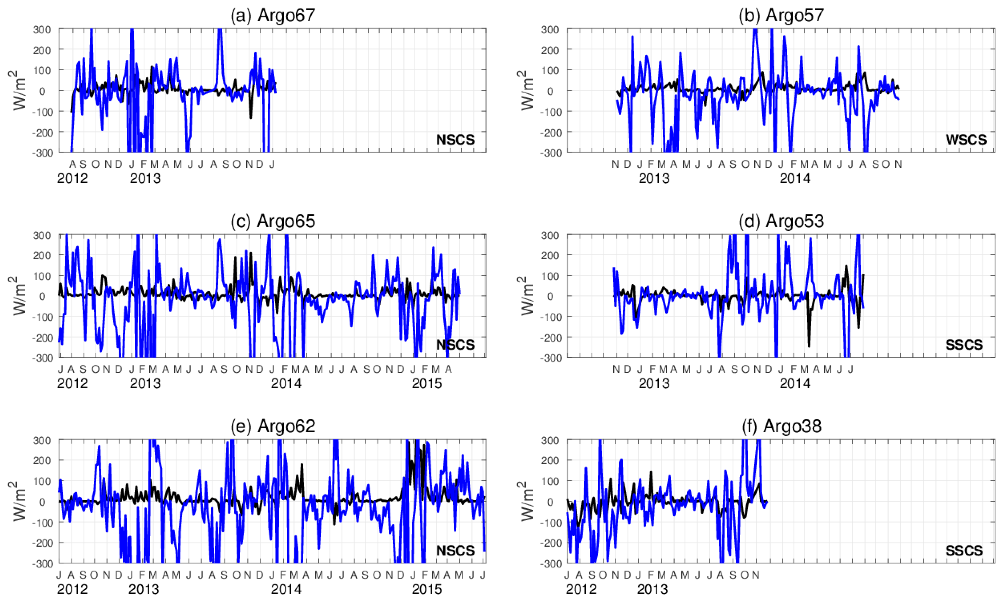
3.1. Residual in the Mixed Layer Heat Budget Equation

Figure 2 shows the variations of monthly means of the temporal change rate of mixed layer heat storage, the sum of net heat flux, horizontal advection, and vertical entrainment, and the residual, and Figure 3 shows those of the net heat flux, the horizontal advection, and the vertical entrainment for the six Argo floats. Although it is difficult to close the heat budget based on observational data [1,32], the tendency of the monthly mean sum of terms is consistent with the rate of mixed layer heat storage. In particular, at Argo67, Argo65, and Argo62, the sum of net heat flux, horizontal advection, and vertical entrainment can explain most of the mixed layer heat variations. Figure 2 also verifies the accuracy of the mixed layer heat budget along the float trajectory, though there are still residuals.

The Argo observed mixed layer heat variation over the SCS shows strong temporal and spatial variability. Mixed layer heat variations have an obvious seasonal cycle. Warming is observed from March to June and then cooling from July to the following February. The maximal warming rate is usually in March whereas the maximal cooling rate is in December–February (Argo67, Argo65, and Argo62), or in June–July (Argo53, Argo38).

The amplitude with the seasonal cycle of heat storage varies spatially. In the NSCS (Argo67, Argo65, and Argo62), the maximum amplitude of the rate of heat storage (black line in Figure 2) can exceed −400 W/m² in winter, whereas it is only 150 W/m² in the SSCS (Argo53 and Argo38). This is related to the distribution of net surface heat flux in the SCS. Moreover, there seems to be a half-yearly cycle of heat storage tendency in Argo53, which is located within the southeastern basin, with the first peak in March and the second peak in October. The heat storage tendency is in qualitative agreement with a previous study over the SCS [12] but with different amplitude. Argo57 moved within an area similar to Box D in Qu [12], and except for November 2013, its time series of heat storage is similar to that in Qu [12]. However, the heat storage of Argo57 is 128.92 W/m² (9.375 × 10⁻⁷ °C/s) in March 2013 and −80.99 W/m² (−6.354 × 10⁻⁷ °C/s) in October 2013, which are larger than the values in Box D in Qu [12] of about 4 × 10⁻⁷ °C/s in April and about −4 × 10⁻⁷ °C/s in October. Argo65 operated in the area within Box A and Argo62 operated near Box B. Their values show similar differences.

The individual terms in Equation (1) are shown in Figure 3 for the six Argo floats. The amplitudes of each term are larger in the NSCS (Argo67, Argo 65, and Argo62) than in the WSCS (Argo57) and SSCS (Argo53 and Argo38). Of all the terms contributing to the heat balance, the net heat flux plays the most significant role in the mixed layer heat variation. Monthly mean heat storage and net heat flux are strongly correlated (correlation coefficient between 0.61 and 0.89, except for Argo38 with 0.4). In the northern Argo floats (Argo67, Argo65, and Argo62), the less net surface heat fluxes result in cooling the ML from October to January the following year, whereas in the southeastern Argo floats (Argo53 and Argo38), the net heat fluxes are positive throughout the year which indicates warming of the ML.

Horizontal heat advection also shows evident differences for each Argo float. Horizontal heat advection fluctuates considerably in the NSCS (Argo67, Argo65, Argo62) and WSCS (Argo57), especially in winter, and reaches −644 W/m² in February 2014. The area where these floats operated is in the range of the SCS WBC, which is a strong seasonal current and carries active eddies along its path [33]. The heat advection in the southeastern SCS is a small term because the local currents are weak. Remarkably, the winter horizontal heat advection varies from year to year. The positive horizontal heat advection warms the ML in winter 2012 as observed by Argo67 and Argo65, whereas Argo62 observes cooling. In the results from Argo62, heat advection is negative in winter 2012 and 2013, but positive in winter 2014. This is caused by complex currents in the WBC, which are discussed in the next section.

Without conspicuous temperature inversions in the SCS, entrainment cools the ML all year in all the studied Argo floats. In the NSCS (Argo67, Argo65, Argo62) and WSCS (Argo57), entrainment is more evident when the northeast monsoon prevails, which favors MLD deepening due to wind stirring and Ekman pumping. On the contrary, entrainment is weaker in other seasons. In the SSCS (Argo53 and Argo38), entrainment is less than −100 W/m² all year.

The residuals in each float are large differently. The residuals fluctuate more widely in NSCS, especially for the season autumn and winter (from October to subsequent February). For example, the residual could reach 627 W/m² in Argo62. The residuals are comparatively smaller in WSCS and SSCS. Residuals increase in winter in WSCS, while in summer in SSCS. The largest amplitudes of residuals are in WSCS and SSCS are 263 W/m² and 262 W/m², respectively. Compared with the monthly mean time series of the mixed layer heat storage rate and the summation of other terms, the residual always varies dramatically along with the present abnormal summation, especially for the winter season in NSCS (Argo67, Argo65, and Argo62). Therefore, residual may come from the calculation of right-hand side of the Equation (1). After all, they cannot be evaluated correctly. More details about the causes of float-to-float differences among seasonal mean residual term will be examined in the next section.

3.2. Annual Mean and Seasonal Variability

Figure 4 displays the annual mean heat storage for the six Argo floats. Because these Argo floats operate over different periods (Table 1), we calculate the annual means for different time periods: From August 2012 to July 2013 for Argo67, from July 2012 to June 2014 for Argo67, from July 2012 to June 2015 for Argo62, from November 2012 to October 2014 for Argo57, from January 2013 to December 2013 for Argo53, and from July 2012 to June 2013 for Argo38. All six Argo floats observe negative annual mean heat storage, meaning that the ML cools.

Because there is much more negative net heat flux observed along the trajectories, the annual mean net heat flux is relatively weak in Argo67 and Argo65, whereas the net surface heat flux is still important term in the budget for other floats. The net heat flux has a substantial positive value in the SSCS, where strong shortwave radiation is a significant contributor all year. The annual mean horizontal heat advection makes a negative contribution to the budget for all the Argo floats, except Argo53. However, the contribution of horizontal advection for Argo53 is the smallest. Entrainment becomes a significant part of the annual mean of the budget because of its persistent cooling of the ML, especially in the NSCS. The annual mean of the residual term varies from float to float. The differences are likely owing to the diverse lengths of the time series used to compute the heat budget.

Table 2. Summer and winter mean in each year of the different terms in the mixed layer heat budget Equation (1). Units are W/m².

Year	Season	Argo	dT	Qnet − Qpen	Advection	Entrainment	Residual
2012	Summer	Argo65	5.36	61.96	53.43	−33.76	−76.27
		Argo62	13.71	57.26	−10.52	−35.13	2.1
		Argo38	−13.63	38.97	−148.88	−60.89	157.16
	Winter	Argo67	−129.05	−155.46	−104.21	−66.2	196.81
		Argo65	−144.61	−125.98	−127.55	−60.58	169.5
		Argo62	−38.17	11.97	−260.87	−70.45	281.18
		Argo57	−77.82	−27.62	25.11	−96.14	20.83
		Argo53	−37.14	35.07	−23.26	−58.81	9.86
		Argo38	−28.64	63.64	−0.63	−18.85	−72.8
2013	Summer	Argo67	−30.78	67.83	36.06	−104.81	−29.86
		Argo65	−33.19	54.92	34.78	−48.41	−74.47
		Argo62	−12.85	41.87	−46.66	−45.67	37.62
		Argo57	−28.06	59.1	−30.34	−35.23	−21.59
		Argo53	−40.15	42.21	1.57	−38.44	−45.49
		Argo38	−30.78	67.83	36.06	−104.81	−29.86
	Winter	Argo65	−146.41	−90.31	−90.34	−71.65	105.9
		Argo62	−224.4	−75.02	−225.25	−119.53	195.39
		Argo57	−44.4	−62.26	3.97	−88.77	102.67
		Argo53	−40.47	45.31	22.2	−30.38	−77.61
2014	Summer	Argo65	−73.29	89.45	6.06	−76.28	−92.52
		Argo62	−14.71	77.03	2.09	−42.33	−51.51
		Argo57	14.05	68.85	−33.53	−66.87	45.6
	Winter	Argo65	−134.09	−108.02	−61.46	−27.11	62.49
		Argo62	−41.03	−59.79	58.32	−65.19	25.63

displays the summer and winter season mean of the different terms in each year. In summer 2012, the net heat flux term controls mainly the heat budget balances in the NSCS (Argo65, Argo62), while heat advection controls in the SSCS (Argo38). Residual is largest in SSCS (Argo38). In winter 2012, large heat loss to air and cold advection make the ML cool evidently in NSCS (Argo67, Argo65) and WSCS (Argo57). Though ML obtains net heat flux, it becomes cooler because of the negative entrainment flux in SSCS. Residuals are large in NSCS while small in WSCS and SSCS. In summer 2013, residuals become mild all the areas. All terms have similar value in NSCS and WSCS. Net heat flux and entrainment terms are the main factors for ML heat balance in SSCS. In winter 2013, large heat loss to air and cold advection are likewise comparable to the situations in winter 2012 but with larger heat loss from entrainment in NSCS. On the contrary, the net heat flux and entrainment terms become important in WSCS and SSCS. Residual is still large in NSCS. In summer and winter 2014, all terms have identical characteristics.

Generally, in summer, the net heat flux term drives mainly the heat budget balances; heat advection and entrainment are the second contributions. However, in winter time, heat advection becomes important as the net heat flux term does in the NSCS. Net heat flux still exerts a major effect on heat storage rate in WSCS and SSCS. Entrainment term seems no difference between summer and winter over the SCS. Residual shows drastic because of volatile heat advection in both summer and winter.

The monthly mean mixed layer heat budget and annual mean of each term show that there is great seasonal variation in the mixed layer heat budget, especially in the net heat flux and horizontal heat advection terms. In next section, we will firstly discuss their seasonal variations between summer and winter in the SCS.

4. Discussion

4.1. Summer And Winter Net Heat Flux

To better resolve the spatial and temporal scales, Figure 5 shows the mean net heat flux fields for the 2012, 2013, and 2014 summers and winters. There are remarkable differences between summer and winter. The net heat flux term warms the entire SCS in summer 2012–2014 with the heating increasing northward (Figure 5a–c) due to the moving northward direct solar radiation. Compared to the stronger heating by the net heat flux term in the northern and western basins, there is always a minimum-value area in the southeastern basin, especially at the northwest of Palawan Island, leading to the striking contrast between the central and NSCS. This phenomenon is due to strengthened evaporation that leads to an increase of latent heat and clouds and thus decreasing the incoming shortwave radiation with the occurrence of the barrier layer [34]. This is why net heat flux is reduced in summer (Figure 4d).

The net heat flux effect for the 2012–2014 winters is dramatically different from that in summer (Figure 5d–f). In winter, the net heat flux term generally cools the northern and western basins but warms the southeastern basin. The intense and cold northeast wind and increasing evaporation in the NSCS lead to more net ocean heat loss. The net heat flux term becomes negative in the northern and central SCS, with values below 200 W/m² in the continental slope region of the NSCS. In the southern and southeastern basin, the net heat flux term still warms the ocean and is stronger than that in summer in the southern part of the basin.

Figure 6 displays the time series of heating contributions decomposed into SWR, LHF, the sum of LWR and SHF. They also vary significantly in the northern study area (Argo67, Argo65, Argo62, and Argo57). The seasonal cycle of SWR changes similarly with the seasonal cycle of the net heat flux (Figure 3). A combination of variations with the solar zenith angle, water vapor, clouds, aerosols, and other parameters, results in large values of SWR in summer, some exceeding 300 W/m², but smaller values in winter. Note that LHF also generally varies in phase with SWR in the northern study area: It increases significantly from summer to winter, as evaporative cooling strengthens because of strong northeast wind over cold waters from Kuroshio intrusion. Therefore, net heat flux becomes smallest during winter in the NSCS (Figure 5a,c,e). SWR and LHF do not show significant seasonal variability in the SSCS (Argo53 and Argo38). In particular, SWR remains around 150 W/m² all year for Argo38. The sum of LWR and SHF is small for all Argo floats and thus has little effect on net heat flux.

4.2. Summer and Winter Horizontal Advection

Figure 7 shows the field of currents and horizontal heat advection for the 2012, 2013, and 2014 summers and winters. Here, we used monthly MLD form SODA 3.3.1 dataset to calculate the horizontal heat advection. In summer, ocean circulation in the SCS is controlled by an anticyclonic gyre (Figure 7a–c). Northward currents flow along the South Vietnam coast, whereas the currents in the eastern basin are very weak as the local wind field is weak and the sea surface is flat. Substantial horizontal heat advection appears in the western and SSCS, especially off the Southeast Vietnam coast. As the southwest monsoon prevails, mixed layer currents (Figure 7a–c) move northward offshore to the middle of Vietnam, forming the anticyclonic South Vietnam eddy. The southwest monsoon blows along the South Vietnam coast, driving coastal upwelling and a cold filament [35], rapidly changing the horizontal heat advection. Currents flowing northeastward with higher temperature waters warm the mixed layer between 7° N and 11° N, whereas to the north of 11° N, the start of the cold filament, the continuing northeast current carries cold water that cools the ML.

In reaction to the strong positive winter monsoon curl, the current field in the SCS changes into a cyclonic gyre with two cyclonic eddies [36]. There is an energetic WBC in the NSCS, especially in winter 2014. Several eddies are still embedded in the basin-scale circulation; for example, the Southern Cyclonic eddy in the SSCS and the West Luzon eddy. Horizontal heat advection also varies over the SCS. Interestingly, horizontal heat advection, unlike the situation in summer, is negative between 7° N and 11° N but is positive north of 11° N in the SSCS. This is due to the effects of the SST gradient and current field. The southward WBC along the East Vietnam coast carries colder sea waters south of 11° N, whereas warmer waters develop north of 11° N because of the warm tongue off the southwest coast of Hainan Island. The reverse heat advection around the center of the West Luzon eddy currents is also due to the local SST gradient [37] associated with the SST front that is aligned from northeast to southwest in the NSCS. The southwestward current to the north of the Luzon cyclonic eddy advects warm waters from the Kuroshio intrusion through the Luzon Strait, whereas the eddy advects cold waters on its south side because of the northwestward current. The heat advection in our results is different from that in Wang et al. [38], which has positive heat advection to the southeast of the Luzon eddy and negative heat advection to its northwest.

Comparing the components in heat advection, we find geostrophic advection is significantly larger than Ekman advection (Figure 8), which differs from results obtained by calculating and averaging over the boxed areas in [7]. Geostrophic advection has larger amplitude in all Argo floats, affected by the eddy activities evident from Argo65 and Argo62. In the northern basin, Ekman advection and geostrophic advection are weak and nearly zero during summer, whereas they fluctuate dramatically from November to February. In contrast, in the SSCS, Ekman advection and geostrophic advection are strong in summer but not in winter. This is because the more northerly Argo floats were located around the SCS WBC where there were many embedded eddies during winter. Currents in the southeastern SCS are not strong even under the influence of the southeast monsoon.

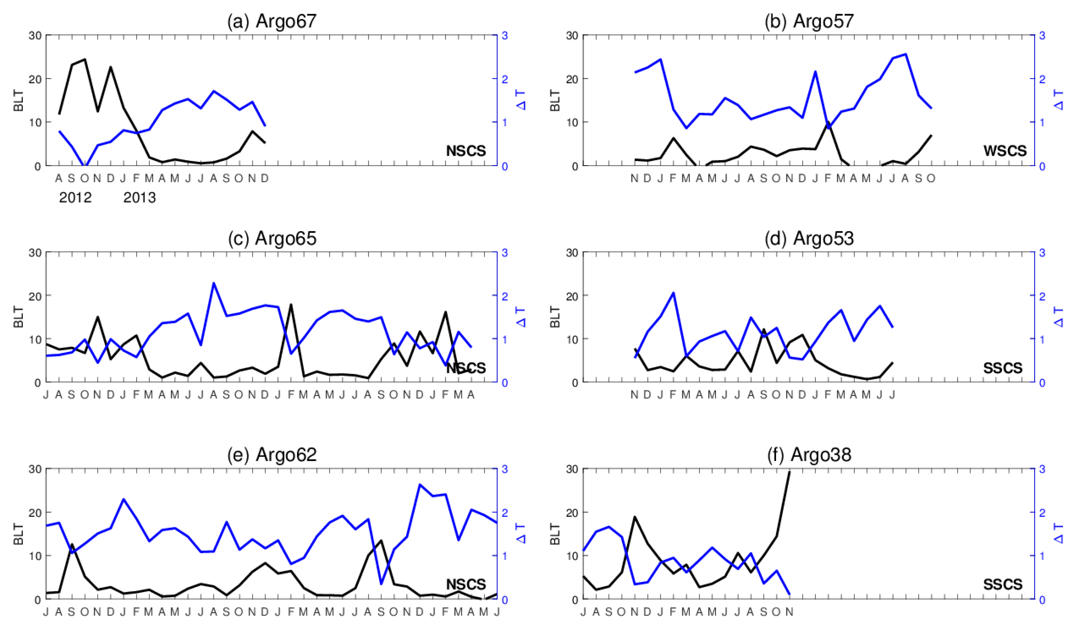
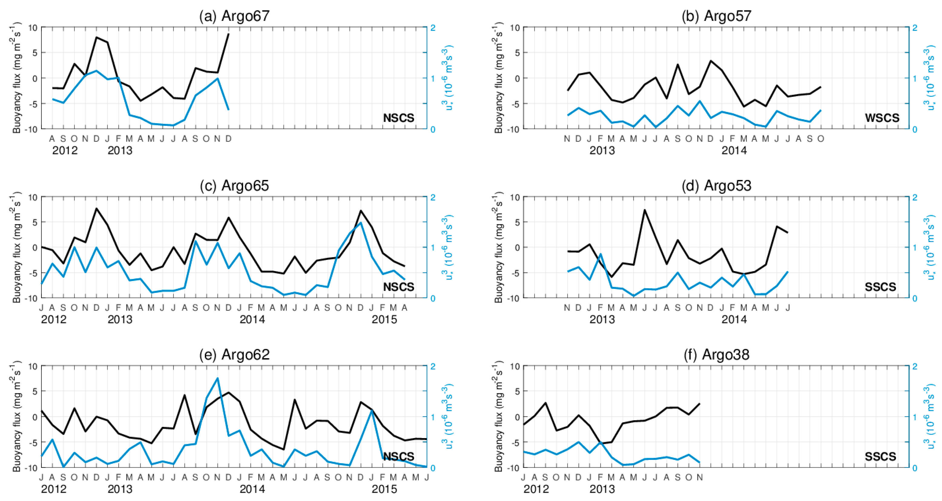
4.3. Possible Impacts on Vertical Entrainment

Figure 4 shows that entrainment is a significant part of the annual mean mixed layer heat balance, and many studies have focused on this contribution. Qu [12] found vertical entrainment could cool the ML when the southwest monsoon prevails. Foltz et al. [1] found that vertical entrainment contributes significantly in tropical Atlantic Ocean. Factors like the barrier layer that influence entrainment have also been studied in many areas apart from the SCS [10,39]. In this section, the entrainment term is decomposed into entrainment rate and the temperature difference $\mathsf{\Delta }T$ between the $T_m$ and $T_h$, and possible impacts on vertical entrainment are discussed.

Monthly mean entrainment, entrainment rate, and $\mathsf{\Delta }T$ of the six Argo floats are shown in Figure 9. Entrainment cooling and its contributions are stronger in Argo67, 65, 62, and 57. Because there are so few temperature inversions in our observations, entrainment always plays a role in cooling the ML.

The entrainment rate increases from late autumn to winter, then decays in spring and summer for Argo67, 65, and 62, whereas the opposite trend is found for Argo53. This may be caused by the seasonal wind field in the SCS. In Argo57 and 38, however, the entrainment rate shows no significant seasonal variations. The temperature difference $\mathsf{\Delta }T$ increases during spring and summer but decreases during autumn and winter for Argo67 and 65. However, the temperature difference for Argo62 varies from year to year. Its magnitude exceeds 1 °C in winter 2012 and 2014 but not in 2013, and it increases more in summer 2014 than in summer 2012 and 2013. These conditions are considered to be the result of local ocean stratification along the trajectory. Seasonal features are not found in $\mathsf{\Delta }\mathrm{T}$ for the other Argo floats.

The complex temporal trends of entrainment rate and $\mathsf{\Delta }T$ contribute to the changes in the entrainment term. However, their correlations are different. The correlation between the entrainment term and the entrainment rate is highest in Argo62 (0.65), but not significant for other floats. The correlation between entrainment and $\mathsf{\Delta }T$ is high in Argo53 and Argo38 (exceeding 0.60), which indicates that the cooling entrainment term is more sensitive to $\mathsf{\Delta }T$ in the southeastern SCS. Looking back at Figure 9, the variation of entrainment is not a function of just rate or temperature difference. We suggest that entrainment rate and temperature difference both have important impacts on entrainment in the SCS.

To study entrainment in more detail, we discuss the causes of the changes of the rate and $\mathsf{\Delta }T$. The entrainment rate consists of the rate of MLD deepening and Ekman suction. The rate of MLD deepening is ten times larger than Ekman pumping in our results (not shown), which differs from the results in Qu [12]. $\mathsf{\Delta }\mathrm{T}$ may be explained in terms of the BLT. There is a barrier layer in the SCS, although it is weaker than that in the western Pacific or Bay of Bengal [26,40]. Figure 10 displays the occurrence of the BL on January 15 2014 from Argo65 observations. Because the BL includes the deepest part of the isothermal layer, the temperature difference $\mathsf{\Delta }T$ is inextricably bound up with the BL (Figure 11). When there is a BL, the temperature of the water underlying the ML is not substantially cooler. Therefore, the entrainment of water beneath the ML causes less heat loss in the ML. Decreasing $\mathsf{\Delta }T$ with strengthening BL is found for all Argo floats. For example, in Argo67 May–October 2013, in Argo57 August 2013–July 2013, in January 2013–July 2014, and so on, $\mathsf{\Delta }T$ was higher as the BL thins than it was in previous months with a thick BL. To a certain extent, the BL may prevent the ML from losing more heat by entrainment.

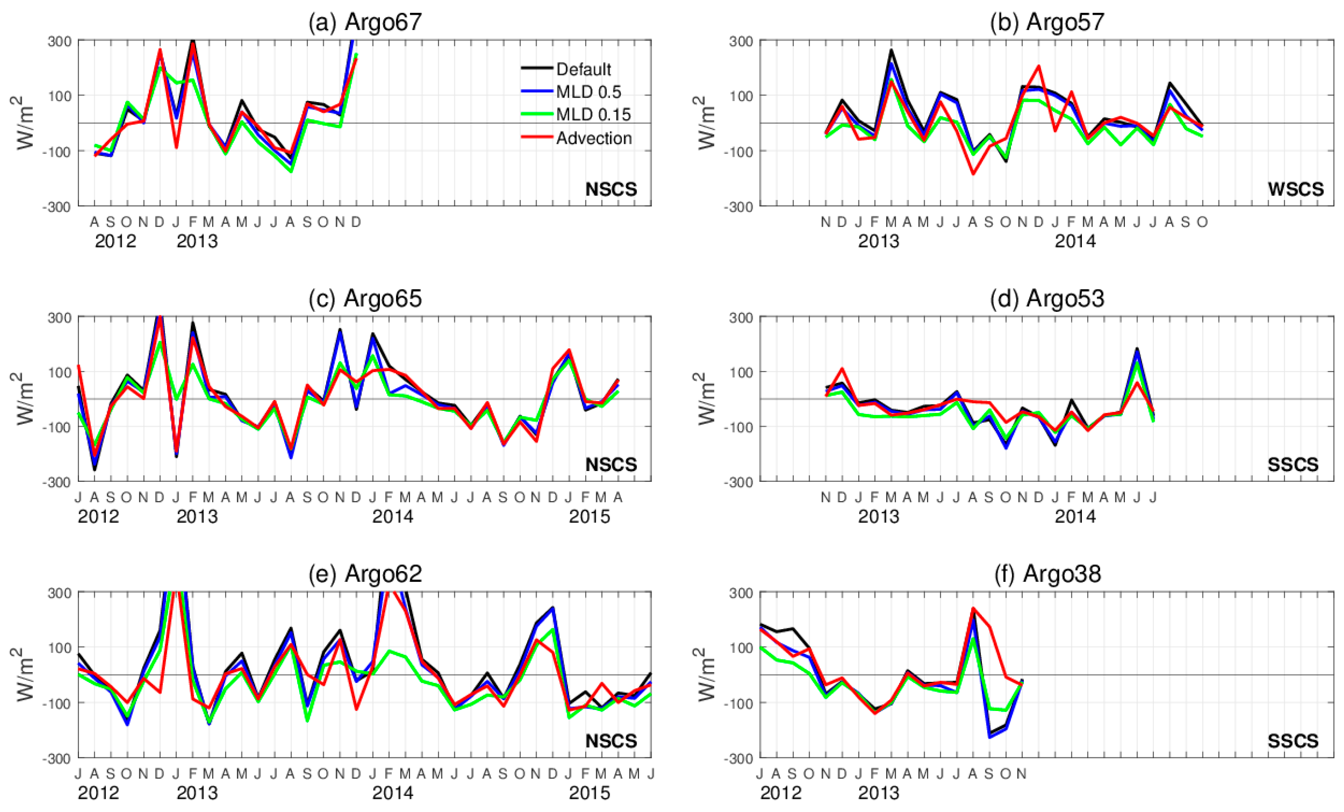
4.4. Possible Causes of the Residual

In Figure 2, there are differences between the mixed layer heat storage rate and the sum of other terms on the right-hand side of the equation except residual. Fluctuations of residuals vary in different area, which are evident in NSCS and comparatively smooth in SSCS. The residual exists in the mixed layer heat budget equation is normal, because it includes the accumulation of errors, and other processes that are unresolved or cannot be parameterized. In this section, we try to study the possible causes of the residual.

One possible reason of the present residual could be the result of the choice of method to calculate the equation [41]. We, therefore, test the sensitivity of residual to other methods. In our study, we calculate the MLD using the temperature criterion of 0.8 °C; calculate the horizontal heat advection using the sum of the Ekman velocity and geostrophic current. For sensitivity analyses, we calculate again the mixed layer heat budget equation by using different MLD based on the temperature criterion of 0.8 °C as well as the density criterion of 0.15 kg m⁻³. In addition, since there are not available daily current velocity datasets, we linearly interpolate the Ocean Surface Current Analyses Real-time (OSCAR) five-day current dataset, which is a NASA funded research project and global surface current database, to daily values. The monthly mean of residuals from different methods are as shown in Figure 12. Compared with the default methods using in our study, there are no evident changes, with consistent phase and similar maximum as well as minimum. The residuals fluctuate more widely in NSCS, while comparatively smooth in WSCS and SSCS. The results suggest that the residuals may be mainly brought out from the unresolved physical processes.

Previous studies suggest that the residual term could be attributed to the vertical turbulent term [41,42]. Thus, we try to study whether the vertical turbulent term could significantly bear on the residual. The vertical turbulent flux is a kind of turbulent kinetic energy transferring from the atmosphere into ML. It is the sum of the cube of the friction velocity ($u_{*}=\sqrt{\tau /\rho }$, where $\tau$ surface wind stress and $\rho$ is the density of seawater) and the surface buoyancy flux, which is defined as B = B_h + B_w ($B_h=\alpha Q/C_p$ and $B_w=\beta \rho S\left(P-E\right)$). Here, $\alpha$ is the coefficient of thermal expansion of seawater, Q is the net surface heat flux, $\beta$ is the coefficient of haline contraction, S is mixed layer salinity, E is evaporation rate, and P is precipitation rate.

Different from Foltz et al. [41] and Wade et al. [42], the monthly mean $u_{*}^3$ and the surface buoyancy flux trends are similar (Figure 13) in our result, which means wind forcing over the SCS usually strengthens with more surface buoyancy flux. They increase strongly in late fall and winter and decrease in spring and summer in the NSCS (Argo67, Argo65, and Argo62) and WSCS (Argo57), while opposite in SSCS (Argo53 and Argo38). Unfortunately, the correlations of monthly $u_{*}^3$ and the surface buoyancy flux with monthly residual are not significant in our result. Therefore, the unconsidered vertical turbulent mixing term is also not the cause leads to the residual.

In Section 3.1, we notice that the residual always fluctuates violently as the present abnormal summation, especially for the winter season in NSCS. However, from monthly mean of all contributions in Equation (1) (Figure 3), the trend of the heat advection term mainly contributes to the change of the summation. Compared the relations between the residual with them in our study (

Table 3. The correlation between residual, net heat flux (Q_net − Q_pen), heat advection, and entrainment.

Sea Area	Argo	Qnet − Qpen	Advection	Entrainment
NSCS	Argo67	−0.67	−0.85	−0.18
	Argo65	−0.42	−0.84	−0.16
	Argo62	−0.21	−0.93	−0.53
WSCS	Argo57	−0.24	−0.67	−0.29
SSCS	Argo53	−0.23	−0.94	−0.48
	Argo38	−0.43	−0.93	−0.61

), we find that the heat advection term has good agreement with the residual in each area. This means that the instability of residual is primarily associated to the heat advection. The net heat flux term and entrainment term only show relative in Argo67 and Argo38 with no more than −0.67 and −0.61 correlation coefficient, respectively.

In our study, the monthly mixed layer heat budget equation is calculated based on the Argo float profiles, which are one-dimensional time series. The interpolation to the Argo float trajectories in calculating the heat advection term may result in errors. Additionally, in Section 4.2, we know that four-day geostrophic advection along the trajectories changes fiercely all over the areas because of the energetic eddy activities and strong wind forcing. The parameterizations of these dynamic processes also induce simulation errors. Therefore, the present residuals may come from the inexact calculation of heat geostrophic advection, other unconsidered missing terms (horizontal heat diffusion and the temperature and horizontal velocity covariance) and unresolved physical ocean dynamic processes.

5. Conclusions

In this study, we investigated the mixed layer heat variation over the SCS using six Argo profiling floats during 2012–2015. We used the same equation as Qiu [22] to compute the mixed layer heat budget. Almost all the terms in the budget equation can be estimated from Argo data and surface reanalysis datasets (TropFlux surface heat flux, ECMWF wind field, CMEMS geostrophic current, and NOAA SST). According to the trajectories of the Argo floats, we divide our study area into three sections (the NSCS, the WSCS, and the southeastern SCS).

Because there are missing observations in the original Argo profiles, we performed quality control of the temperature and salinity profiles. After this, the heat budget assessment for the six Argo floats was discussed. We used NOAA SST to represent the mixed layer temperature, and the sum of Ekman and geostrophic current to represent the mixed layer current. Although there are still differences, the sum of net heat flux, heat advection, and entrainment is largely consistent with monthly mean mixed layer heat storage (Figure 2). Mixed layer heat storage is usually positive from March to June as the ML warms, and then cooling occurs from July to February.

The amplitude of all terms in the equation varies spatially. The amplitude in the northern area is large, mostly in the range of −300 to 150 W/m², while it is smaller in the southern area. All terms in the heat budget equation have similar temporal and spatial differences (Figure 3). Net heat flux has a strong seasonal cycle for Argo67, 65, 62, and 57, and a semi-seasonal cycle for Argo53 and 38. Net heat flux is highly consistent with mixed layer storage for all Argo floats, but other terms cannot be neglected. Horizontal heat advection shows more dramatic changes during winter in the NSCS (Argo67, 65, 62, and 57), but conversely in summer in SSCS (Argo53 and 38). Without conspicuous temperature inversions in the SCS, entrainment cools the ML all year for all the Argo floats in our study. We also calculated the annual mean heat budget of the six Argo floats. Our results show that the most important term in the heat budget equation is entrainment in the NSCS and net heat flux in the SSCS.

To study the seasonal variation in more detail, we examined the spatial distribution of the net heat flux and horizontal heat advection of the SCS in summer and winter 2012–2014 (Figure 5 and Figure 7). In summer, net heat flux is positive all over the SCS, but increases with latitude, whereas it decreases to negative values in the northern and central SCS in winter. Currents and heat advection are very weak, except in the western basin of the SCS in summer, but they become stronger during winter. Horizontal heat advection due to eddy current activities is significant. Analysis of the evolution of the surface heat flux and horizontal advection shows that short wave radiation and geostrophic current play important roles in net heat flux and heat advection, respectively (Figure 6 and Figure 8). The entrainment term in our results is influenced by both temperature difference and entrainment rate. Moreover, the rate of MLD deepening makes the major contribution to entrainment rate; the existence of a BL could account for the reductions in temperature differences that then decrease the entrainment cooling. The residual analysis finds out that the choice of method to calculate the MLD, the choice of current data, and the vertical turbulent mixing are not the reasons for the residual, but inexact calculation of heat geostrophic advection and the other missing terms and unresolved physical ocean dynamic processes are.

Because there are errors associated with surface heat fluxes and sampling, incomplete observational data (for example, for current measurements), and errors in simulation, the residual term for some Argo floats is noticeably large. Though the mixed layer budget analysis by Argo data remains a challenge, the results of this study may improve our understanding of mixed layer variations in the SCS. We suggest that future studies about mixed layer heat balance analysis could combine observation from using Argo floats data with numerical experiment [43]. Furthermore, improved flux estimates and longer-term and more precise observations in the SCS will help us understand more clearly how the ocean heat budget influences air–sea exchange.

References

1. Qu, T.; Du, Y.; Sasaki, H. South China Sea throughflow: A heat and freshwater conveyor. Geophys. Res. Lett. 2006, 33. [Google Scholar] [CrossRef]
2. Xiao, F.A.; Wang, D.X.; Zeng, L.L.; Liu, Q.Y.; Zhou, W. Contrasting changes in the sea surface temperature and upper ocean heat content in the South China Sea during recent decades. Clim. Dyn. 2019, 53, 1597–1612. [Google Scholar] [CrossRef]
3. Zeng, L.; Schmitt, R.W.; Li, L.; Wang, Q.; Wang, D.J.C.D. Forecast of summer precipitation in the Yangtze River Valley based on South China Sea springtime sea surface salinity. Clim. Dyn. 2019, 1–15. [Google Scholar] [CrossRef]
4. Zeng, L.L.; Liu, W.T.; Xue, H.J.; Xiu, P.; Wang, D.X. Freshening in the South China Sea during 2012 revealed by Aquarius and in situ data. J. Geophys. Res. Ocean. 2014, 119, 8296–8314. [Google Scholar] [CrossRef]
5. Zeng, L.L.; Wang, D.X.; Xiu, P.; Shu, Y.Q.; Wang, Q.; Chen, J. Decadal variation and trends in subsurface salinity from 1960 to 2012 in the northern South China Sea. Geophys. Res. Lett. 2016, 43, 12181–12189. [Google Scholar] [CrossRef]
6. Zeng, L.L.; Chassignet, E.P.; Schmitt, R.W.; Xu, X.B.A.; Wang, D.X. Salinification in the South China Sea Since Late 2012: A Reversal of the Freshening Since the 1990s. Geophys. Res. Lett. 2018, 45, 2744–2751. [Google Scholar] [CrossRef]
7. Kuo, N.J.; Zheng, Q.N.; Ho, C.R. Satellite observation of upwelling along the western coast of the South China Sea. Remote Sens. Environ. 2000, 74, 463–470. [Google Scholar] [CrossRef]
8. Liu, Q.Y.; Jiang, X.; Xie, S.P.; Liu, W.T. A gap in the Indo-Pacific warm pool over the South China Sea in boreal winter: Seasonal development and interannual variability. J. Geophys. Res. Ocean. 2004, 109, 07012. [Google Scholar] [CrossRef]
9. Liu, W.T.; Xie, X.S. Spacebased observations of the seasonal changes of South Asian monsoons and oceanic responses. Geophys. Res. Lett. 1999, 26, 1473–1476. [Google Scholar] [CrossRef]
10. Shaw, P.; Chao, S. Surface circulation in the South China Sea. Deep-Sea Res. Part I Oceanogr. Res. Pap. 1994, 41, 1663–1683. [Google Scholar] [CrossRef]
11. Qu, T. Upper-Layer Circulation in the South China Sea. J. Phys. Oceanogr. 2000, 30, 1450–1460. [Google Scholar] [CrossRef]
12. Qu, T. Role of ocean dynamics in determining the mean seasonal cycle of the South China Sea surface temperature. J. Geophys. Res. Atmos. 2001, 106, 6943–6955. [Google Scholar] [CrossRef]
13. Yang, H.; Qinyu, L.; Davis, X. On the Upper Oceanic Heat Budget in the South China Sea: Annual Cycle. Adv. Atmos. Sci. 1999, 16, 619–629. [Google Scholar] [CrossRef]
14. Song, W.; Lan, J.; Qinyan, L.; Sui, D.; Zeng, L.; Wang, D. Decadal variability of heat content in the South China Sea inferred from observation data and an ocean data assimilation product. Ocean Sci. 2014, 10, 135–139. [Google Scholar] [CrossRef] [Green Version]
15. Thompson, B.; Tkalich, P. Mixed layer thermodynamics of the Southern South China Sea. Clim. Dyn. 2013, 43, 2061–2075. [Google Scholar] [CrossRef]
16. Thompson, B.; Tkalich, P.; Malanotte-Rizzoli, P.; Fricot, B.; Mas, J. Dynamical and thermodynamical analysis of the South China Sea winter cold tongue. Clim. Dyn. 2015, 47, 1629–1646. [Google Scholar] [CrossRef] [Green Version]
17. Wang, C.; Wang, W.; Wang, D.; Wang, Q. Interannual variability of the South China Sea associated with El Niño. J. Geophys. Res. 2006, 111. [Google Scholar] [CrossRef]
18. Tan, W.; Wang, X.; Wang, W.; Wang, C.; Zuo, J. Different Responses of Sea Surface Temperature in the South China Sea to Various El Nino Events during Boreal Autumn. J. Clim. 2016, 29, 1127–1142. [Google Scholar] [CrossRef]
19. Foltz, G.; Schmid, C.; Lumpkin, R. Seasonal Cycle of the Mixed Layer Heat Budget in the Northeastern Tropical Atlantic Ocean. J. Clim. 2013, 26, 8169–8188. [Google Scholar] [CrossRef]
20. Girishkumar, M.S.; Ravichandran, M.; McPhaden, M.J. Temperature inversions and their influence on the mixed layer heat budget during the winters of 2006–2007 and 2007–2008 in the Bay of Bengal. J. Geophys. Res. Ocean. 2013, 118, 2426–2437. [Google Scholar] [CrossRef]
21. Zeng, L.; Wang, D.; Chen, J.; Wang, W.; Chen, R. SCSPOD14, a South China Sea physical oceanographic dataset derived from in situ measurements during 1919–2014. Sci. Data 2016, 3, 160029. [Google Scholar] [CrossRef] [PubMed]
22. Qiu, B. Interannual Variability of the Kuroshio Extension System and Its Impact on the Wintertime SST Field. J. Phys. Oceanogr. 2000, 30, 1486–1502. [Google Scholar] [CrossRef]
23. Kara, A.B.; Rochford, P.A.; Hurlburt, H.E. Mixed layer depth variability and barrier layer formation over the North Pacific Ocean. J. Geophys. Res. Ocean. 2000, 105, 16783–16801. [Google Scholar] [CrossRef] [Green Version]
24. Sprintall, J.; Tomczak, M. Evidence of the barrier layer in the surface-layer of the tropics. J. Geophys. Res. Ocean. 1992, 97, 7305–7316. [Google Scholar] [CrossRef]
25. Zeng, L.; Du, Y.; Xie, S.-P.; Wang, D. Barrier layer in the South China Sea during summer 2000. Dyn. Atmos. Ocean. 2009, 47, 38–54. [Google Scholar] [CrossRef] [Green Version]
26. Zeng, L.; Wang, D. Seasonal variations in the barrier layer in the South China Sea: Characteristics, mechanisms and impact of warming. Clim. Dyn. 2017, 48, 1911–1930. [Google Scholar] [CrossRef]
27. Kumar, B.P.; Vialard, J.; Lengaigne, M.; Murty, V.S.N.; Mcphaden, M.J. TropFlux: Air-sea fluxes for the global tropical oceans—description and evaluation. Clim. Dyn. 2012, 38, 1521–1543. [Google Scholar] [CrossRef]
28. Sweeney, C.; Gnanadesikan, A.; Griffies, S.M.; Harrison, M.J.; Rosati, A.J.; Samuels, B.L. Impacts of Shortwave Penetration Depth on Large-Scale Ocean Circulation and Heat Transport. J. Phys. Oceanogr. 2005, 35, 1103–1119. [Google Scholar] [CrossRef] [Green Version]
29. Kaufman, Y.J.; Koren, I.; Remer, L.A.; Tanre, D.; Ginoux, P.; Fan, S. Dust transport and deposition observed from the Terra-Moderate Resolution Imaging Spectroradiometer (MODIS) spacecraft over the Atlantic ocean. J. Geophys. Res. Atmos. 2005, 110. [Google Scholar] [CrossRef]
30. Michel, S.; Chapron, B.; Tournadre, J.; Reul, N. Sea surface salinity variability from a simplified mixed layer model of the global ocean. Ocean Sci. Discuss. 2007, 4, 41–106. [Google Scholar] [CrossRef]
31. Berrisford, P.; Dee, D.P.; Poli, P.; Brugge, R.; Mark, F.; Manuel, F.; Kållberg, P.W.; Kobayashi, S.; Uppala, S.; Adrian, S. The ERA-Interim Archive Version 2.0; ECMWF: Shinfield Park, Reading, UK, 2011. [Google Scholar]
32. Hayes, S.P.; Chang, P.; McPhaden, M.J. Variability of the Sea Surface Temperature in the Eastern Equatorial Pacific During 1986–1988. J. Geophys. Res. Ocean. 1991, 96, 10553–10566. [Google Scholar] [CrossRef]
33. Wang, D.; Liu, Q.; Xie, Q.; He, Z.; Zhuang, W.; Shu, Y.; Xiao, X.; Hong, B.; Wu, X.; Sui, D. Progress of regional oceanography study associated with western boundary current in the South China Sea. Chin. Sci. Bull. 2013, 58, 1205–1215. [Google Scholar] [CrossRef] [Green Version]
34. Tian, Y.Q.; Pan, A.J. A preliminary study on the special and temporal distribution feature of the summertime net heat flux in the northwest waters off the Palawan Island and its formation mechanism. J. Oceanogr. Taiwan Strait 2012, 31, 540–548. [Google Scholar]
35. Xie, S.-P.; Xie, Q.; Wang, D.; Liu, W.T.L. Summer upwelling in the South China Sea and its role in regional climate variations. J. Geophys. Res. Ocean. 2003, 108. [Google Scholar] [CrossRef] [Green Version]
36. Wyrtki, K. Physical oceanography of the Southeast Asian waters. In NAGA Report; Scripps Institution of Oceanography: La Jolla, CA, USA, 1961; Volume 2, p. 195. [Google Scholar]
37. Chow, C.H.; Liu, Q. Eddy effects on sea surface temperature and sea surface wind in the continental slope region of the northern South China Sea. Geophys. Res. Lett. 2012, 39, 2601. [Google Scholar] [CrossRef]
38. Wang, G.; Li, J.; Wang, C.; Yan, Y. Interactions among the winter monsoon, ocean eddy and ocean thermal front in the South China Sea. J. Geophys. Res. Ocean. 2012, 117, 08002. [Google Scholar] [CrossRef]
39. Vialard, J.; Delecluse, P. An OGCM Study for the TOGA decade. Part I: Role of salinity in the physics of the Western Pacific fresh pool. J. Phys. Oceanogr. 1998, 28, 1071–1088. [Google Scholar] [CrossRef]
40. Liang, Z.; Xie, Q.; Zeng, L.; Wang, D. Role of wind forcing and eddy activity in the intraseasonal variability of the barrier layer in the South China Sea. Ocean Dyn. 2018, 68, 363–375. [Google Scholar] [CrossRef]
41. Foltz, G.R.; Vialard, J.; Kumar, B.P.; McPhaden, M.J. Seasonal Mixed Layer Heat Balance of the Southwestern Tropical Indian Ocean. J. Clim. 2010, 23, 947–965. [Google Scholar] [CrossRef]
42. Wade, M.; Caniaux, G.; Dupenhoat, Y. Variability of the Mixed Layer Heat Budget in the Eastern Equatorial Atlantic during 2005–2007 as inferred from Argo Floats. J. Geophys. Res. Ocean. 2010, 116. [Google Scholar] [CrossRef]
43. De Boisseson, E.; Thierry, V.; Mercier, H.; Caniaux, G. Mixed layer heat budget in the Iceland Basin from Argo. J. Geophys. Res. Ocean. 2010, 115. [Google Scholar] [CrossRef] [Green Version]
Figure 1. (af) Trajectories of six Argo floats used in this study (blue lines represent the tracks of Argo floats, green and red dots represent the start and end locations, respectively). Variation of (g) temperature (°C) and (h) salinity in the upper 150 m from Argo62. Blue contours in (g) and (h) are mixed layer depths.
Sustainability 11 05429 g001
Figure 2. Monthly mean mixed layer heat storage rate (black), the sum (magenta) of first 3 terms on the right-hand side of the mixed layer heat budget Equation (1), and residual (dashed) for (a) Argo67, (b) Argo57, (c) Argo65, (d) Argo53, (e) Argo62, and (f) Argo38. Units are W/m2.
Sustainability 11 05429 g002
Figure 3. Monthly mean mixed layer heat storage rate (shading, red: Warming, and blue: Cooling) and individual terms on the right-hand side of the mixed layer heat budget Equation (1) (lines, magenta: Net heat flux term; black: Horizontal advection term; gray: Vertical entrainment term) for (a) Argo67, (b) Argo57, (c) Argo65, (d) Argo53, (e) Argo62, (f) Argo38. Units are W/m2.
Sustainability 11 05429 g003
Figure 4. Pie chart with annual mean percentage of the different terms on the right-hand side of the mixed layer heat budget Equation (1) (slices, magenta: Net heat flux term; black: Horizontal advection term; gray: Vertical entrainment term; white: Residual terms) for (a) Argo67, (b) Argo65, (c) Argo62, (d) Argo57, (e) Argo53, and (f) Argo38. The heat storage annual mean percentage is indicated by the red number in the lower-left corner.
Sustainability 11 05429 g004
Figure 5. Summer (ac) and winter (df) mean net heat flux term (W/m2) for (left) 2012, (middle) 2013, and (right) 2014.
Sustainability 11 05429 g005
Figure 6. Time series of heating contribution (W/m2) by shortwave radiation (red line), latent heat flux (blue line), sum of longwave radiation and sensible heat flux (gray line) terms for (a) Argo67, (b) Argo57, (c) Argo65, (d) Argo53, (e) Argo62, and (f) Argo38.
Sustainability 11 05429 g006
Figure 7. Summer (ac) and winter (df) mean horizontal advection term (shading; W/m2) and mixed layer averaged currents (vectors; m/s) for (left) 2012, (middle) 2013, and (right) 2014.
Sustainability 11 05429 g007
Figure 8. Time series of advective contributions from Ekman advection (black line), and geostrophic advection (blue line) terms for (a) Argo67, (b) Argo57, (c) Argo65, (d) Argo53, (e) Argo62, and (f) Argo38.
Sustainability 11 05429 g008
Figure 9. Monthly mean vertical entrainment term (black line; W/m2), the entrainment rate (blue solid line; 10−5 m/s), and the temperature difference (∆T; blue dashed line, °C) between T (the mixed layer temperature) and Th (the temperature of water entrained into the mixed layer (ML), taken to be the temperature at 5 m below the mixed layer depth (MLD)) for (a) Argo67, (b) Argo57, (c) Argo65, (d) Argo53, (e) Argo62, and (f) Argo38.
Sustainability 11 05429 g009
Figure 10. Vertical profiles of temperature (red), salinity (blue), and density (black) on January 15 2014 of Argo65. Blue (red) dashed line indicates MLD (isothermal layer depth (ILD)).
Sustainability 11 05429 g010
Figure 11. Monthly mean of the temperature difference between T and Th (∆T; blue line, °C) and barrier layer thickness (black line; m) for (a) Argo67, (b) Argo57, (c) Argo65, (d) Argo53, (e) Argo62, and (f) Argo38.
Sustainability 11 05429 g011
Figure 12. Monthly mean of residual term calculated with default methods (black line), MLD computed using the temperature criterion of 0.5 °C (blue line), and density criterion of 0.15 kg m−3 (green line), Ocean Surface Current Analyses Real-time (OSCAR) current dataset (red line) for (a) Argo67, (b) Argo57, (c) Argo65, (d) Argo53, (e) Argo62, and (f) Argo38.
Sustainability 11 05429 g012
Figure 13. Monthly mean of the surface buoyancy flux (black) and the cube of the friction velocity (blue) for (a) Argo67, (b) Argo57, (c) Argo65, (d) Argo53, (e) Argo62, and (f) Argo38.
Sustainability 11 05429 g013