Optimal Control Strategy for Variable Air Volume Air-Conditioning Systems Using Genetic Algorithms

Abstract

This study is aimed at developing a real-time optimal control strategy for variable air volume (VAV) air-conditioning in a heating, ventilation, and air-conditioning (HVAC) system using genetic algorithms and a simulated large-scale office building. The two selected control variables are the settings for the supply air temperature and the duct static pressure to provide optimal control for the VAV air-conditioning system. Genetic algorithms were employed to calculate the optimal control settings for each control variable. The proposed optimal control conditions were evaluated according to the total energy consumption of the HVAC system based on its component parts (fan, chiller, and cold-water pump). The results confirm that the supply air temperature and duct static pressure change according to the cooling load of the simulated building. Using the proposed optimal control variables, the total energy consumption of the building was reduced up to 5.72% compared to under ‘normal’ settings and conditions.

1. Introduction

Heating, ventilation, and air-conditioning (HVAC) systems constitute a significant portion of the energy consumption of many buildings [1,2,3]. Researchers have tried to determine a methodology to reduce such HVAC energy consumption [2,4] and, among the developed methodologies, genetic algorithms (GAs) are widely used in various fields and are known to be suitable for solving complex optimization problems, especially when large amounts of data and parameters are involved [5,6]. Therefore, GAs (a type of machine learning technique) are applicable for the optimization of complex configurations of systems such as buildings [7]. Extensive research has been conducted to optimize the thermal performance of buildings and reduce energy consumption, particularly that of the building’s HVAC system [8]. Recent studies have shown that optimization methods that use GAs can save energy in HVAC systems and improve energy efficiency [9,10,11]. Researchers have carried out analyses of the changes in the energy consumption of HVAC systems with respect to building design parameters [9] and have optimized HVAC system design based on simulations [10].

The performance of buildings and their HVAC systems is influenced in real time due to factors such as temperature and humidity of the outside air, operation modes and patterns, and others. In order to implement efficient operations and effectively control a building’s HVAC system, the HVAC system must be operated and controlled by optimal control variables (settings) in real time that correspond to the changes in load usage according to the external environment. Preferably, such optimal operation and control can be implemented without additional costs for updating the system [12].

The typical local controls in a valuable air volume (VAV) air-conditioning system rely on static pressure control, supply air temperature, and outdoor air flow [13,14,15]. These local controls have an effect on the indoor comfort and energy consumption in the system. The appropriate controls can be achieved by adopting indoor loads and outdoor conditions in real time. Local controls in a VAV system have traditionally been implemented using controllers with values derived from traditional control strategies such as setpoint reset, proportional integral derivative (PID), and model predictive control (MPC) [16,17,18].

HVAC systems are comprised of many components and subsystems (e.g., fans, chillers, pumps, ductwork, pipes, heat exchangers, etc.). In this research, an office building was used as the reference building in which the HVAC system was modeled and simulated. The optimal control variables were derived from genetic algorithms (GAs) and are proposed to mitigate energy consumption and optimize the performance of HVAC systems in large-scale office buildings. The calculated optimal control variables/settings were input to a variable air volume (VAV) air-conditioning system at one-hour intervals. GAs were employed to analyze the changes in the calculated optimal control variables which, in turn, were used to operate the modeled system. Using this process, energy savings were calculated and compared with the energy consumption under previous ‘normal’ (compared to ‘optimal’) operating conditions.

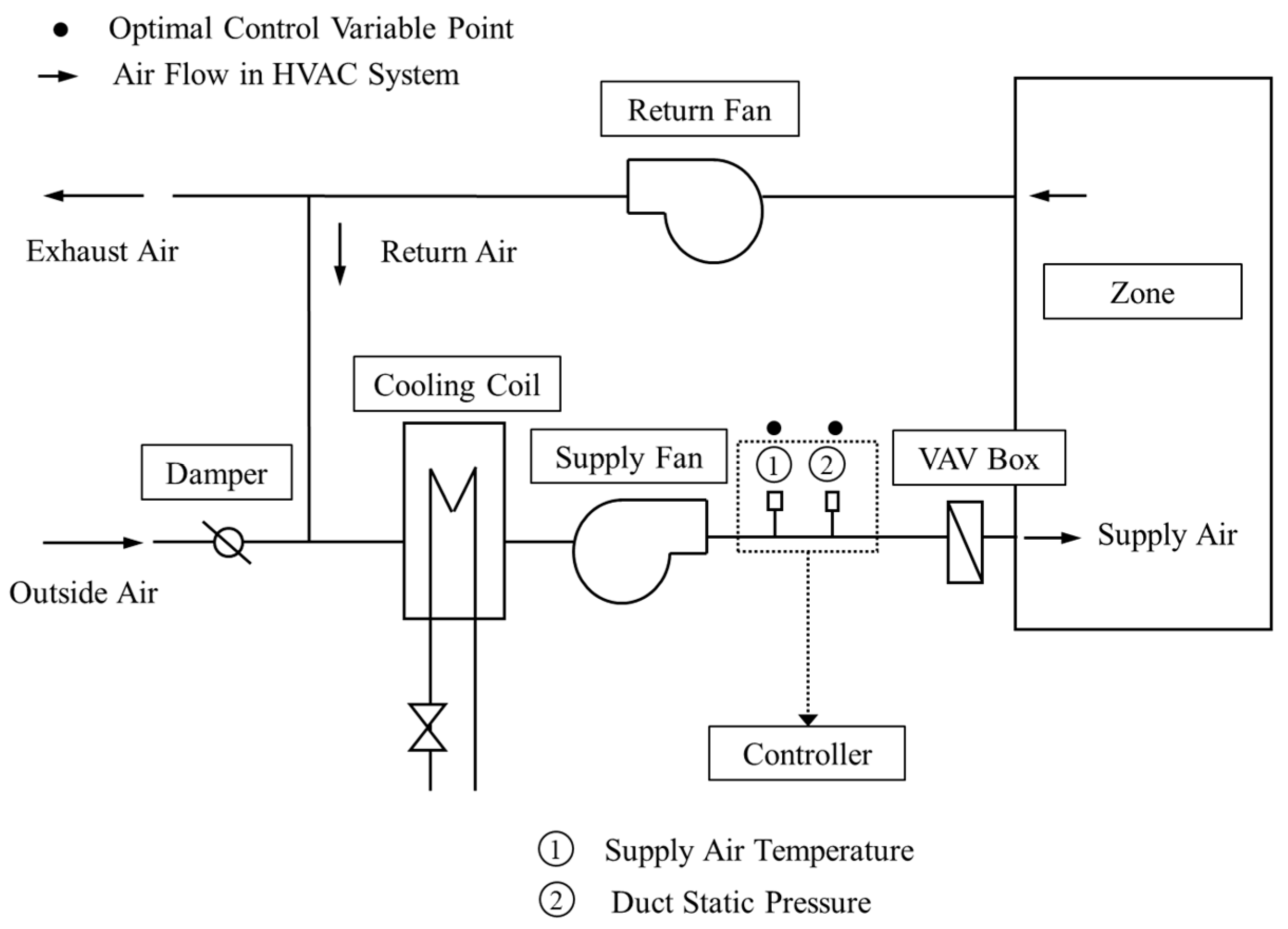
2. Generation of Simulated Reference Building and Description of VAV System

Among the standard buildings found in the Commercial Prototype Building Models proposed by the United States Department of Energy’s Building Energy Codes Program [19,20] and ANSI/ASHRAE/IES Standard 90.1 [21] for standardized energy assessment, the category of Large Office Buildings [22] was selected as the building type to generate the required input data for this study. The input values for the reference building were modified to reflect the usage profile of a large office building in Korea [23]. To fit the simulation program, weather information was obtained by modifying test reference year (TRY) data, which are the standard weather data for the Seoul area.

Table 1. Simulation Conditions for Reference Large-Scale Office Building. HVAC: heating, ventilation, and air-conditioning.

Component	Features
Weather data and site location	Test reference year (TRY) Seoul (latitude: 37.57°N, longitude: 126.97°E)
Building type	Large-scale office building
Total building area (m2)	46,320
Hours simulated (hour)	8760
Envelope insulation (m2K/W)	External wall 0.35, roof 0.213, external window 1.5
Window-to-wall ratio (%)	40
Setting (°C)	Cooling 26, heating 20
Internal gain	Lighting 10.76 (W/m2), people 18.58 (m2/person), plug and process 10.76 (W/m2)
HVAC sizing	Autocalculated (software to be determined)
HVAC operation schedule	7:00–18:00

presents the main boundary conditions that were used in the proposed simulation model to acquire data.

The building and its HVAC system were simulated using EnergyPlus version 8.9.0 (U.S. Department of Energy, Washington, DC, USA) [24]. The outputs, which include energy consumption, were generated from EnergyPlus and include quantities for flow, temperature, and pressure at each node in the building’s system. The HVAC system modeled in this study has an air handling unit that provides a VAV system to each room and a freezer that can be used also as a heat source in cold weather. Numerous controllable settings are required to manage a VAV system, from heating and cooling temperature settings and minimum airflow rate settings at the zone level to the minimum outside airflow, supply air temperature, and duct static pressure settings at the system level [25]. Among the various controllable variables in an HVAC system, the settings for supply air temperature and duct static pressure are selected specially for the study as the control variables in the VAV air-conditioning system. Figure 1 describes a typical VAV HVAC system that includes the control setting locations for the supply air temperature and duct static pressure.

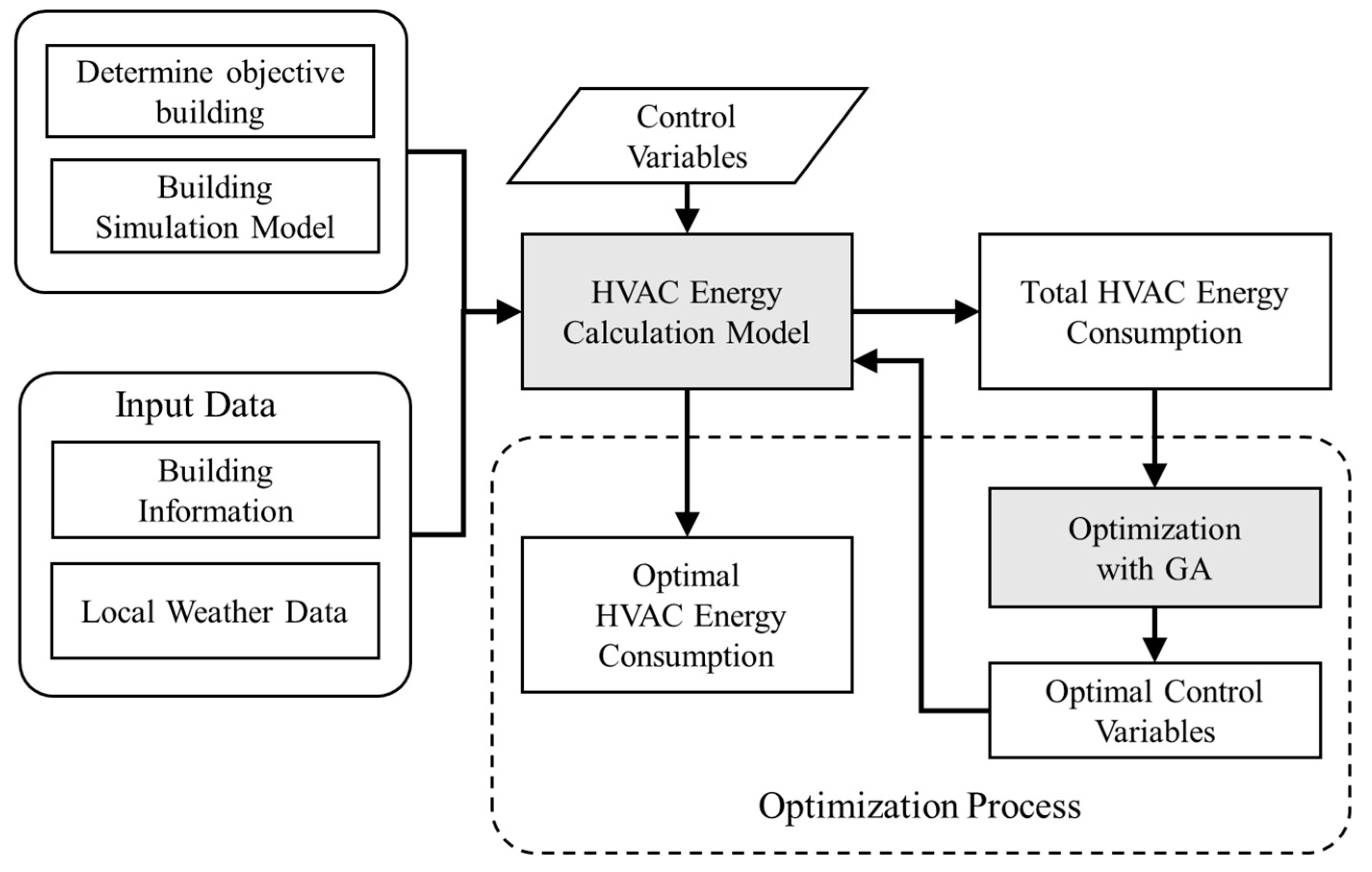
3. Optimal Control Using Genetic Algorithms

In this study, GAs were used to derive optimal control parameters for an optimized control operation. The objective function is the total energy consumption of the HVAC system. First, an energy calculation model for the HVAC system is needed to implement a GA whose objective function is the energy consumption of the HVAC system. The numerical model for calculating the energy of an HVAC system references an existing calculation model and several input variables, including controlled and uncontrolled variables [26,27]. The numerical models to determine energy consumption of three components (fan, chiller, and cold-water pump) in the HVAC system are addressed as follows.

Fan Power Model:

$$Q_z=q_s/1.21\left(t_z-t_s\right),$$

(1)

$$Q_{sys}={\displaystyle \sum }_{i=1}^n{Q}_{z}i,$$

(2)

$$P_t=P_s+C\times {\left(Q_{sys}\right)}^2,$$

(3)

$$P_{fan}=Q_{sys}\times P_t/n_f,$$

(4)

where $Q_z$ is zone air flow (m³/h), $q_s$ is zone sensible load (kW) $t_z$ is zone temperature (°C), $t_s$ is supply air temperature (°C), $Q_{sys}$ is total system air flow (m³/h), n is number of zone, $P_s$ is duct static pressure (Pa), $C$ is flow coefficient (dimensionless), $P_t$ is fan total pressure (Pa), $n_f$ is fan total efficiency (%).

Chiller Power Model:

$$\mathrm{PLR}=q_{ct}/q_{nominal}\times R_f,$$

(5)

$$P_{chiller}=P_{ref}\times CAPFT\times EIRFT\times EIRPLR,$$

(6)

$$P_{ref}=q_{ref}/CO{P}_{ref},$$

(7)

where $\mathrm{PLR}$ is part-load ratio, $q_{ct}$ is system cooling coil load (kW), $q_{nominal}$ is chiller nominal capacity, refrigeration ton (RT), $\mathrm{CAPFT}$ is a curve that represents the capacity factor as a function of evaporator and condenser temperatures, $\mathrm{EIRFT}$ is a curve that represents the energy input ratio to cooling output factor as a function of evaporator and condenser temperatures, $\mathrm{EIRPLR}$ is a curve that represents the energy input ratio factor as a function of part-load ratio, $q_{ref}$ is chiller capacity at reference conditions (reference temperatures and flow rates) (kW), and $CO{P}_{ref}$ is a reference coefficient of performance (W/W).

Pump Power Model:

$$Q_w=q_{ct}/C_w\times {\gamma }_w\times \left(t_{wr}-t_w\right),$$

(8)

$$P_{pump}=Q_w\times H_t/n_p,$$

(9)

where $Q_w$ is chilled water flow rate (L/s), $C_w$ is specific heat capacity of water 4.19 (kJ/kg°C), ${\gamma }_w$ is density of water (1000 kg/m³), $t_{wr}$ is chilled water return temperature (°C), $t_w$ is chilled water temperature (°C), $H_t$ is total pump head (Pa), and $n_p$ is pump total efficiency (%).

The input values that are needed to calculate the energy consumption of the HVAC system are derived from the outputs of the building simulation. The next step is to derive the optimal control variables using GA that gives a set of optimal or potential solutions to a problem. Each solution in the population is referred to as an individual. A generation is a new population of individuals that is created each time [28]; the optimization algorithm is repeated to determine the most optimal solution. Figure 2 presents a flow chart that describes the optimization process to determine optimal control settings using GAs.

The GAs used for the energy calculation model and optimization of the HVAC system were programmed using MATLAB R2018a and the toolbox in MATLAB, respectively. The hot season (from May to September) in Seoul, Korea, was used as the analysis period for calculating the energy consumption of the HVAC system. The total energy consumption of the HVAC system during the hot season is the sum of the energy consumption of three components (fan, chiller, and cold-water pump) in the HVAC system [29]. Total energy consumption can be calculated using Equation (10).

$$P_{total}=P_{fan}+P_{chiller}+P_{pump},$$

(10)

where P is energy consumption. In practice, the setting values need to be selected within a controllable range for real-world applications. The upper and lower limits were set according to the general design conditions of the building and the literature [30,31,32]. The air supply temperature was selected to be between approximately 12 and 19 °C, and the duct static pressure was set to be between approximately 250 and 620 Pa.

Table 2. Control Variables at Fixed Settings and Control Range.

Case	Control Variable
	Supply Air Temp. (°C)	Duct Static Pressure (Pa)
‘Normal’ (Non-optimal) Control Operation	12.8	474
Optimal Control Operation (Range)	Calculate GA (12–19)	Calculate GA (250–620)

shows the design settings for the two control variables (supply air temperature and duct static pressure) and the control range for the variables.

4. Results and Discussion

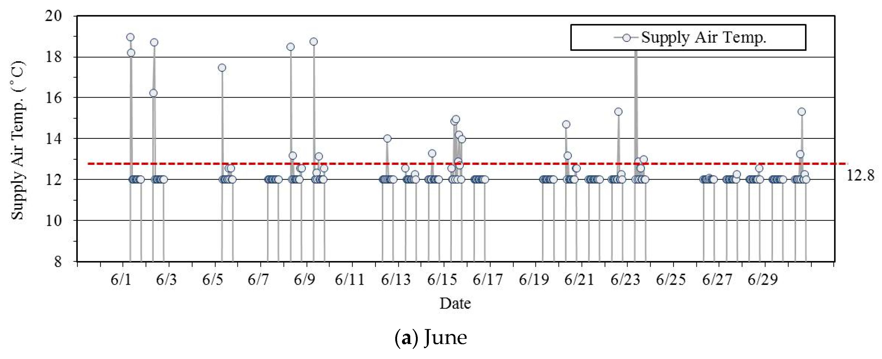
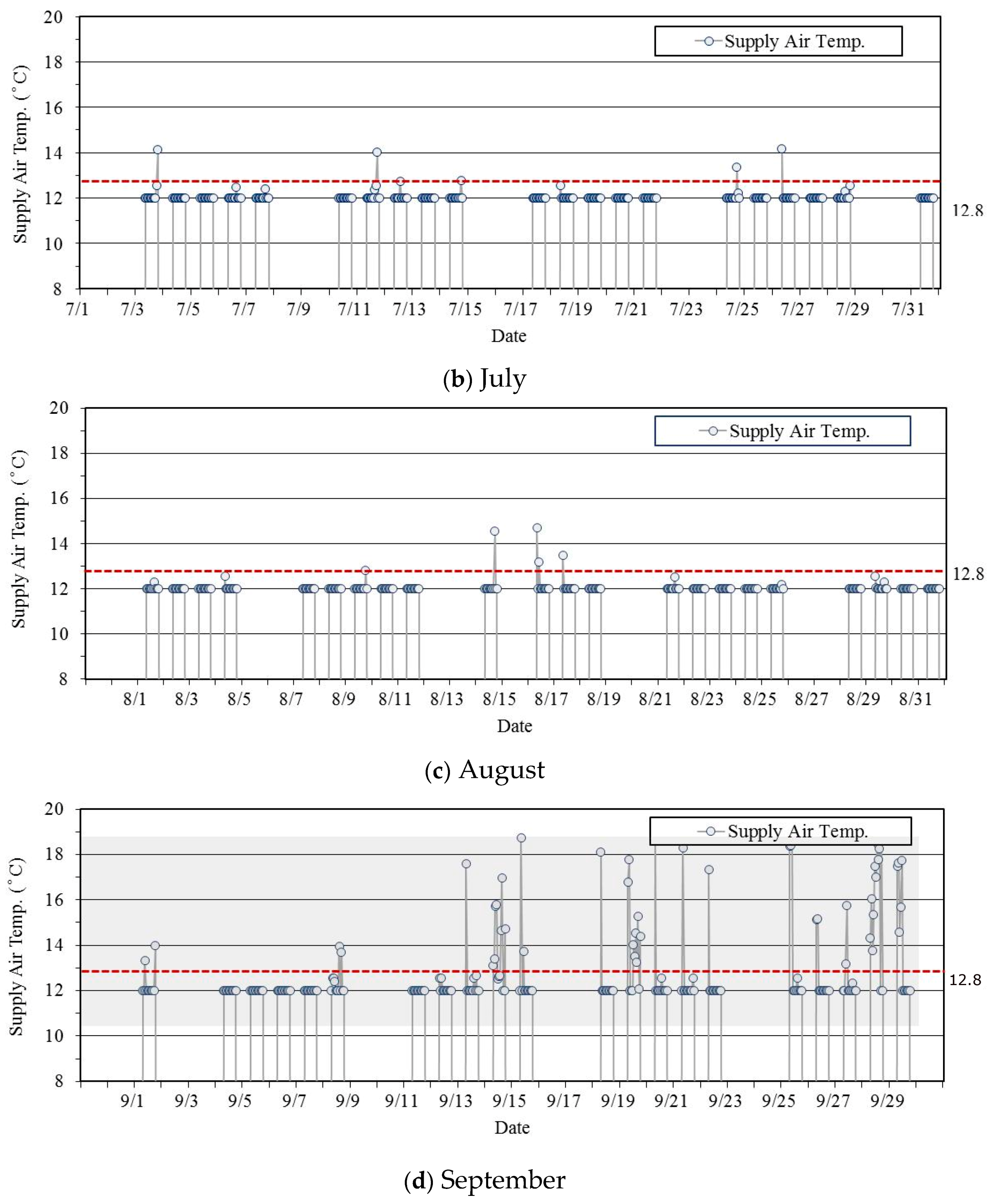
4.1. Effects of Changes in Supply Air Temperature

Figure 3 shows the changes in supply air temperature according to the time series during the optimal control operation from June through September. In June and September, the supply air temperature changes frequently, as shown in Figure 3a,d, but in July and August (the hottest months), the supply air temperature is set as low as 12 °C, as shown in Figure 3b,c. If the supply air temperature is maintained continuously at about 12 °C during normal operations, including July and August, the flow rate of the cold water that circulates in the cooling coil increases, which leads to an increase in the load rate of the refrigerator and an increase in the circulation of the cold water in the cold-water circulation pump, thereby increasing the energy consumption of the system that supplies the cooling source.

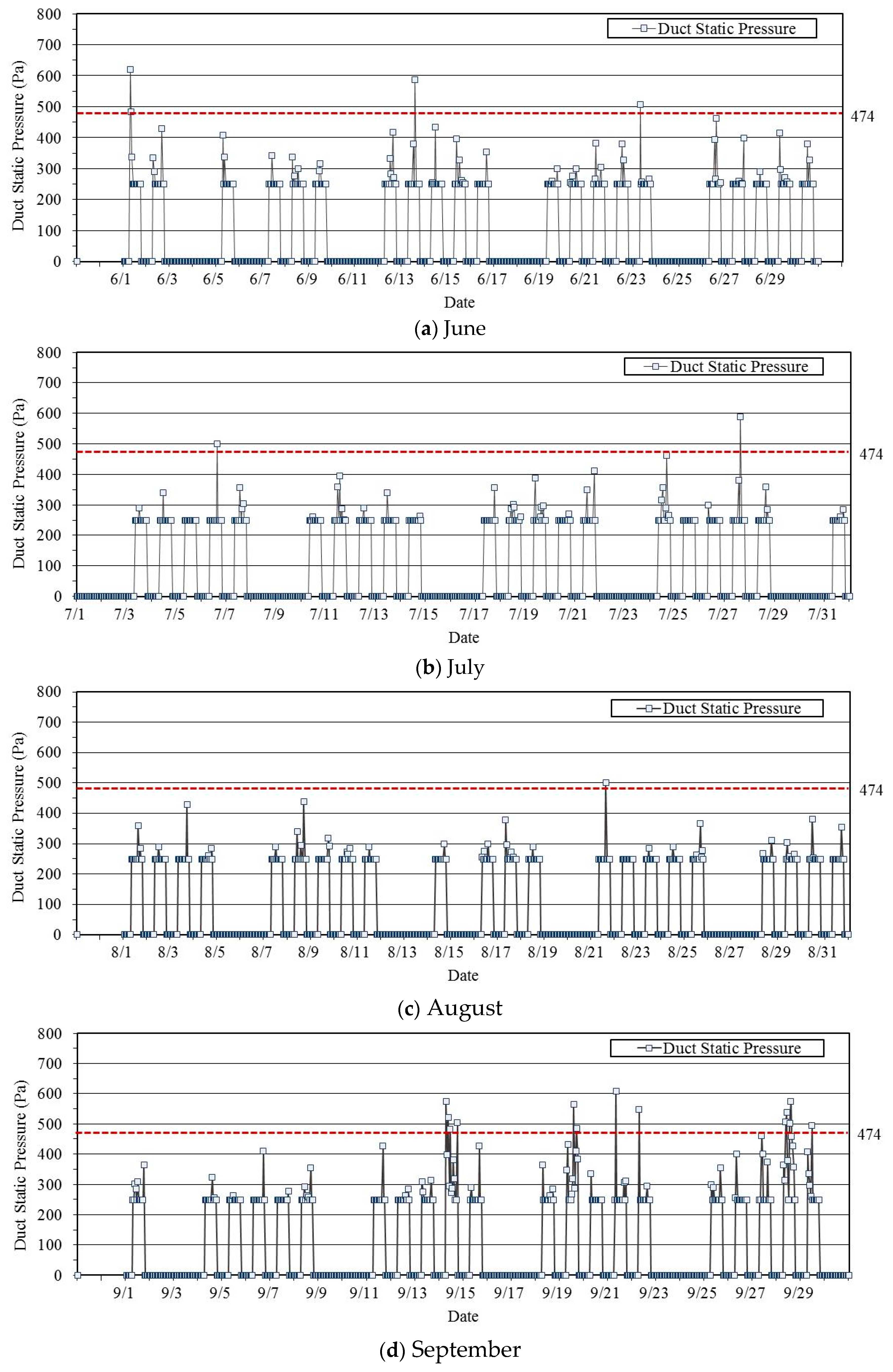
4.2. Effects of Changes in Duct Static Pressure

Figure 4 shows the changes in duct static pressure according to the time series during the optimal control period from June through September. Duct static pressure in the optimal control operation mode is lower than 474 Pa and was kept constant during normal operations. The GA discovered energy savings for the fan by supplying less air than the existing air volume by keeping the static pressure low on the air supply side. However, any reduction in airflow that is due to low static pressure can also cause problems such as the temporary deterioration of indoor air quality, even when the required outdoor air intake for the design is satisfied. Hence, for practical design, ways to maintain proper indoor air quality must also be considered.

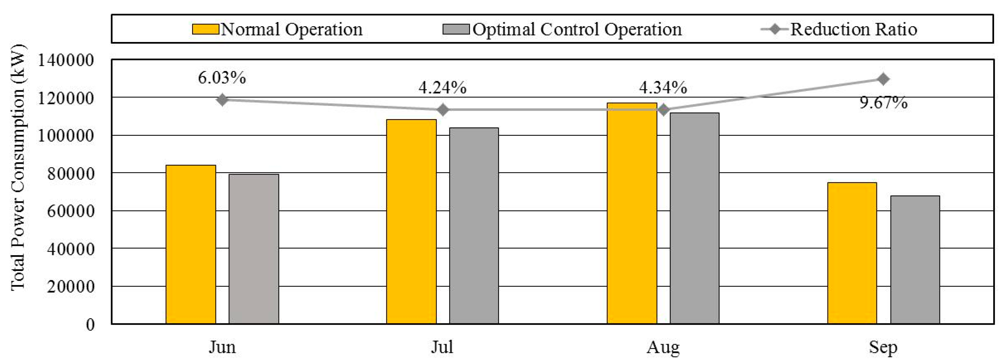
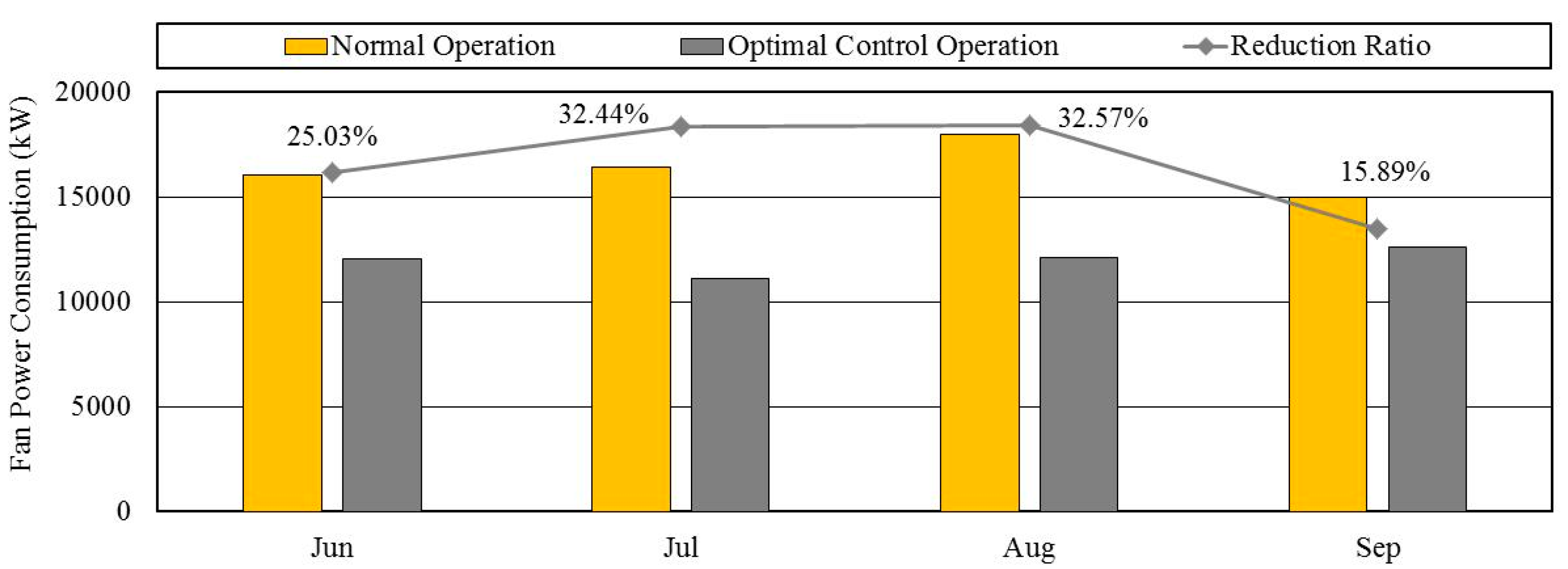
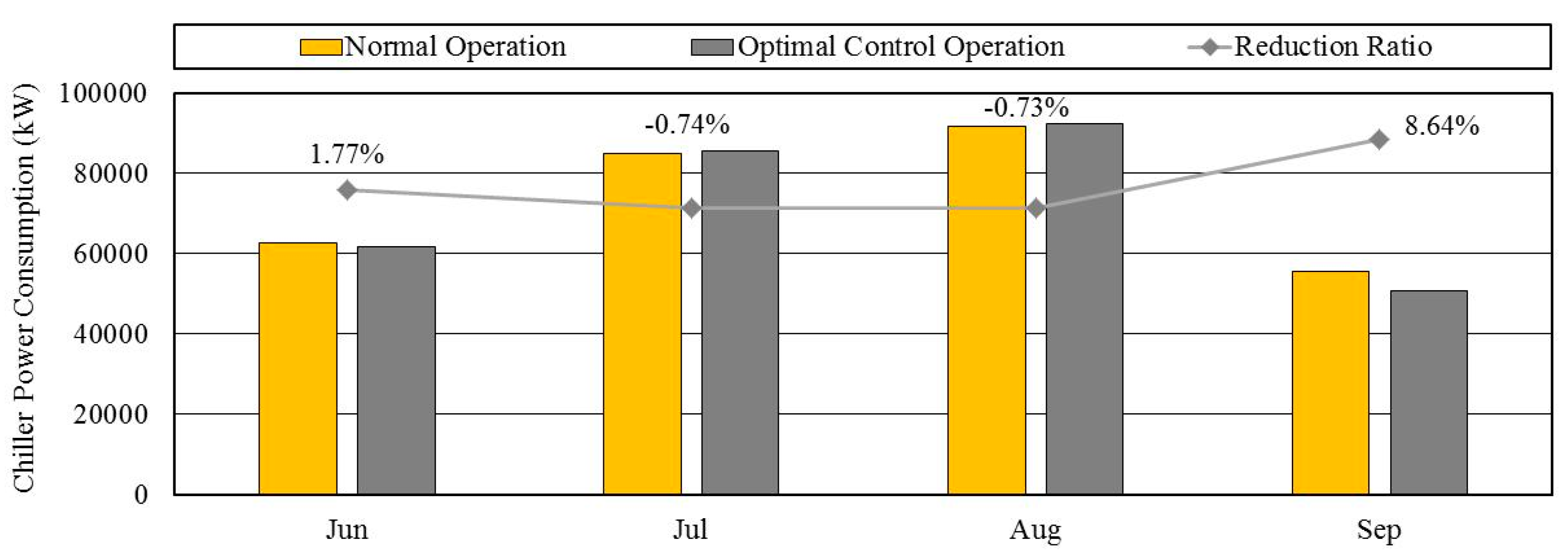
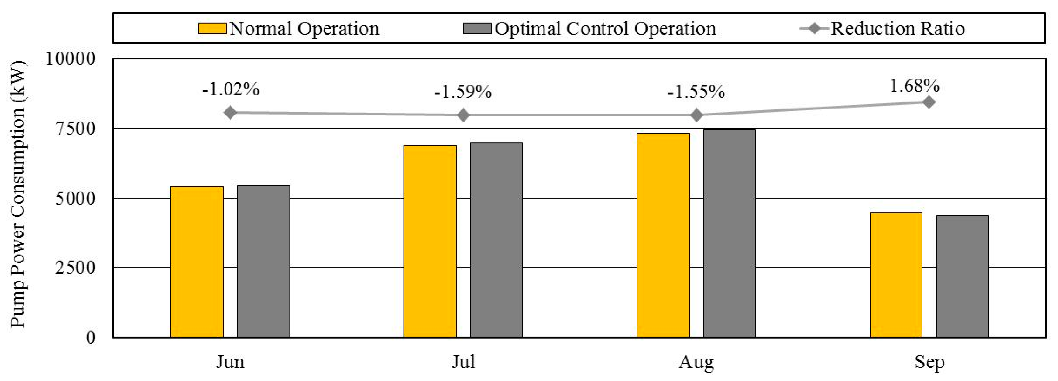
4.3. Comparison of Energy Consumption Levels

Figure 5 presents a comparison of monthly energy consumption with respect to normal operation mode versus optimal operation mode. The total amount of energy saved in July and August when the outside temperature is relatively high is about 4%, and is up to 9.7% in September. The rate of the total cooling energy consumption during the period of analysis from June through September was reduced from 384,296 kW in normal operation mode to 362,309 kW in optimal operation mode, which represents 5.7% in energy savings. The control value changes in the time series according to the changes in outside air conditions and the cooling load. The total energy consumption is calculated as the sum of the separate energy consumption of the fan, chiller, and cold-water pump. The effects of energy consumption for each of these three components in the HVAC system also were analyzed, as discussed in the next three subsections.

(1) Energy consumption of fan

Figure 6 shows the energy consumption and savings rates of the fan in the HVAC system during the cooling period from June through September with respect to operation mode. The results indicate that energy consumption is reduced by at least 15.9–32.6% per month. The energy savings are due to the low duct static pressure, which leads to low static pressure for the fan. The energy consumption of the fan during the cooling months was reduced from 65,449 kW in normal operation mode to 47,865 kW in optimal operation mode, which is a reduction of about 26.9% energy consumption.

(2) Energy consumption of chiller

Figure 7 shows the energy consumption and savings rates of the chiller in the HVAC system during the cooling period from June through September with respect to operation mode. In June and September, the chiller energy consumption decreased by 1.8% and 8.6%, respectively, but the chiller energy consumption increased by about 0.7% in July and August when the outside air temperature and the cooling load were both high. During the cooling period from June through September, the chiller energy consumption decreased by 1.6% from 294,820 kW in normal control mode to 290,213 kW in optimal control mode. Thus, no significant difference was evident in the reduction rate of the energy consumption of the chiller with regard to whether it operated in normal control mode or in optimal control mode.

(3) Energy consumption of cold-water pump

Figure 8 shows the energy consumption and savings rates of the cold-water pump in the HVAC system during the cooling period from June through September with respect to operation mode. The energy consumption of the cold-water circulation pump increased by about 1%, except in September. When the supply air temperature is maintained at a temperature lower than about 0.8 °C compared to the temperature in normal control mode, the flow rate of the cold water that circulates in the cooling coil increases, which results in an increase in the energy consumption of the cold-water pump. The cooling period from June through September saw a 0.9% increase from 24,028 kW in normal control mode to 24,213 kW in optimal control mode.

5. Conclusions

The optimal control strategy proposed in this study uses an objective function as the energy consumption in a GA. Then, GAs are used to select the supply air temperature and duct static pressure as the control variables/settings to operate a VAV system in real time. The following results were obtained from this study.

The proposed optimal control operation was evaluated based on changes in the optimal control variables and energy savings in a simulated HVAC system in a reference large-scale office building. As the two optimal control operations, the air supply temperature was kept as low as 12 °C, which is below the system design value of 12.8 °C, and the duct static pressure was kept at a value lower than the system design value of 474 Pa.

When the low temperature and low pressure were outputs from the GAs, the total energy consumption was reduced by 5.7%, the fan energy consumption was reduced by 26.9%, the chiller energy consumption was reduced by 1.6%, and the cold-water pump energy consumption showed a mere 0.9% increase. However, low supply air temperatures and low air flow rates can cause conditions such as internal condensation in the system or ductwork, cold drafts, and temporary deterioration of the indoor air quality during HVAC operation. Therefore, these possible outcomes need to be addressed when optimizing HVAC system design.

If the energy consumption of the fan unit takes up a large portion of the configuration of the HVAC system, then even more energy savings should be achieved using the proposed method.

Several variables can be controlled in supplying the heat/cooling source, such as the cold-water supply temperature, cold-water flow rate, and cooling the water in the chiller, so further research is required for optimizing HVAC systems using various control settings.

References

1. Navarro, L.; De Gracia, A.; Colclough, S.; Browne, M.; McCormack, S.J.; Griffiths, P.; Cabeza, L.F. Thermal energy storage in building integrated thermal systems: A review. Part 1. Active storage systems. Renew. Energy 2016, 88, 526–547. [Google Scholar] [CrossRef]
2. Homod, R.Z. Analysis and optimization of HVAC control systems based on energy and performance considerations for smart buildings. Renew. Energy 2018, 126, 49–64. [Google Scholar] [CrossRef]
3. Chua, K.J.; Chou, S.K.; Yang, W.M.; Yan, J. Achieving better energy-efficient air conditioning—A review of technologies and strategies. Appl. Energy 2013, 104, 87–104. [Google Scholar] [CrossRef]
4. Ahmed, M.S.; Mohamed, A.; Homod, R.Z.; Shareef, H.; Sabry, A.H.; Khalid, K.B. Smart plug prototype for monitoring electrical appliances in Home Energy Management System. In Proceedings of the 2015 IEEE Student Conference on Research and Development (SCOReD), Kuala Lumpur, Malaysia, 13–14 December 2015; pp. 32–36. [Google Scholar]
5. Bentley, P. An introduction to evolutionary design by computers. In Evolutionary Design by Computers; Morgan Kaufmann Publishers: San Francisco, CA, USA, 1999; pp. 1–73. [Google Scholar]
6. Goldberg, D.E.; Holland, J.H. Genetic algorithms and machine learning. Mach. Learn. 1988, 3, 95–99. [Google Scholar] [CrossRef]
7. Evins, R. A review of computational optimisation methods applied to sustainable building design. Renew. Sustain. Energy Rev. 2013, 22, 230–245. [Google Scholar] [CrossRef]
8. Li, T.; Shao, G.; Zuo, W.; Huang, S. Genetic algorithm for building optimization: State-of-the-art survey. In Proceedings of the 9th International Conference on Machine Learning and Computing, Singapore, 24–26 February 2017; pp. 205–210. [Google Scholar]
9. Bichiou, Y.; Krarti, M. Optimization of envelope and HVAC systems selection for residential buildings. Energy Build. 2011, 43, 3373–3382. [Google Scholar] [CrossRef]
10. Seo, J.; Ooka, R.; Kim, J.T.; Nam, Y. Optimization of the HVAC system design to minimize primary energy demand. Energy Build. 2014, 76, 102–108. [Google Scholar] [CrossRef]
11. Satrio, P.; Mahlia, T.M.I.; Giannetti, N.; Saito, K. Optimization of HVAC system energy consumption in a building using artificial neural network and multi-objective genetic algorithm. Sustain. Energy Technol. Assess. 2019, 35, 48–57. [Google Scholar]
12. Ashrae, A. ASHRAE Handbook- Heating, Ventilating, and Air-conditioning (HVAC) Applications; ASHRAE: New York, NY, USA, 2011. [Google Scholar]
13. Tukur, A.; Hallinan, K.P. Statistically informed static pressure control in multiple-zone VAV systems. Energy Build. 2017, 135, 244–252. [Google Scholar] [CrossRef]
14. Wang, G.; Song, L. Air handling unit supply air temperature optimal control during economizer cycles. Energy Build. 2012, 49, 310–316. [Google Scholar] [CrossRef]
15. Nassif, N. Performance analysis of supply and return fans for HVAC systems under different operating strategies of economizer dampers. Energy Build. 2010, 42, 1026–1037. [Google Scholar] [CrossRef]
16. Rahnama, S.; Afshari, A.; Bergsøe, N.C.; Sadrizadeh, S. Experimental study of the pressure reset control strategy for energy-efficient fan operation–Part 1: Variable air volume ventilation system with dampers. Energy Build. 2017, 139, 72–77. [Google Scholar] [CrossRef]
17. Moradi, H.; Setayesh, H.; Alasty, A. PID-Fuzzy control of air handling units in the presence of uncertainty. Int. J. Therm. Sci. 2016, 109, 123–135. [Google Scholar] [CrossRef]
18. Afram, A.; Janabi-Sharifi, F. Theory and applications of HVAC control systems–A review of model predictive control (MPC). Build. Environ. 2014, 72, 343–355. [Google Scholar] [CrossRef]
19. Building Energy Modeling 101: Stock-Level Analysis Use Case. Available online: https://www.energy.gov/eere/buildings/articles/building-energy-modeling-101-stock-level-analysis-use-case (accessed on 19 September 2019).
20. Field, K.; Deru, M.; Studer, D. Using DOE commercial reference buildings for simulation studies. Proc. SimBuild 2010, 4, 85–93. [Google Scholar]
21. ASHRAE. Energy Standard for Buildings Except Low-Rise Residential Buildings, ANSI/ASHRAE/IESNA Standard 90.1-2010; ASHRAE: New York, NY, USA, 2010. [Google Scholar]
22. Deru, M.; Field, K.; Studer, D.; Benne, K.; Griffith, B.; Torcellini, B.; Liu, B.; Halverson, M.; Winiarski, D.; Rosenberg, M.; et al. U.S. Department of Energy Commercial Reference Building Models of the National Building Stock (NREL/TP-5500-46861); National Renewable Energy Laboratory: Lakewood, CO, USA, 2011. [Google Scholar]
23. Korea Energy Agency. Building Energy Efficiency Rating System Regulation; Korea Energy Agency: Yongin City, Gyeonggi-Do, Korea, 2018. [Google Scholar]
24. U.S. Department of Energy. EnergyPlus Version 8.9.0 Documentation Input Output Reference; U.S. Department of Energy: Washington, DC, USA, 2018.
25. Raftery, P.; Li, S.; Jin, B.; Ting, M.; Paliaga, G.; Cheng, H. Evaluation of a cost-responsive supply air temperature reset strategy in an office building. Energy Build. 2018, 158, 356–370. [Google Scholar] [CrossRef] [Green Version]
26. Tesiero, R.C., III. Intelligent Approaches for Modeling and Optimizing HVAC Systems. Ph.D. Thesis, North Carolina Agricultural and Technical State University, Greensboro, NC, USA, 2014. [Google Scholar]
27. Seong, N. Optimization of Energy Consumption for Central HVAC System based Building Energy Management System Using Genetic Algorithm. Ph.D. Thesis, Gachon University, Seongnam-si, Gyeonggi-do, Korea, 2019. [Google Scholar]
28. Ahmad, M.W.; Mourshed, M.; Yuce, B.; Rezgui, Y. Computational Intelligence Techniques for HVAC Systems: A review. In Building Simulation; Tsinghua University Press: Beijing, China, 2016; pp. 359–398. [Google Scholar]
29. Ahn, B.C.; Mitchell, J.W. Optimal control development for chilled water plants using a quadratic representation. Energy Build. 2001, 33, 371–378. [Google Scholar] [CrossRef]
30. Hong, G.; Kim, B.S. Development of a Data-Driven Predictive Model of Supply Air Temperature in an Air-Handling Unit for Conserving Energy. Energies 2018, 11, 407. [Google Scholar] [CrossRef]
31. Taylor, S.T. VAV System Duct Main Design. ASHRAE J. 2019, 61, 54–60. [Google Scholar]
32. Rahnama, S.; Afshari, A.; Bergsøe, N.C.; Sadrizadeh, S.; Hultmark, G. Experimental study of the pressure reset control strategy for energy-efficient fan operation–Part 2: Variable air volume ventilation system with decentralized fans. Energy Build. 2018, 172, 249–256. [Google Scholar] [CrossRef]
Figure 1. Diagram of typical variable air volume (VAV) air-conditioning system and setting controls.
Sustainability 11 05122 g001
Figure 2. Flow chart of energy analysis model for HVAC system using genetic algorithms.
Sustainability 11 05122 g002
Figure 3. Supply air temperature changes during optimal control mode for (a) June, (b) July, (c) August, and (d) September.
Sustainability 11 05122 g003aSustainability 11 05122 g003b
Figure 4. Duct static pressure changes during optimal control mode for (a) June, (b) July, (c) August, and (d) September.
Sustainability 11 05122 g004
Figure 5. Monthly energy consumption comparison between normal operation mode and optimal operation mode for June through September.
Sustainability 11 05122 g005
Figure 6. Comparison of fan energy consumption between normal operation mode and optimal operation mode for June through September.
Sustainability 11 05122 g006
Figure 7. Comparison of chiller power consumption between normal operation mode and optimal operation mode for June through September.
Sustainability 11 05122 g007
Figure 8. Comparison of cold-water pump energy consumption between normal operation mode and optimal operation mode for June through September.
Sustainability 11 05122 g008