Efficiency of the EU Environmental Policy in Struggling with Fine Particulate Matter (PM_2.5): How Agriculture Makes a Difference?

Abstract

Fine particulate matter (PM_2.5) emissions are an important global issue as air pollutants lead to approximately 7 million deaths per year (World Health Organization). In an attempt to combat this global threat, countries in the European Union (EU) allocate relatively large funds for environmental policies. The main goal of this paper is to assess the long-term efficiency of the EU countries’ environmental policy in reducing the pressure of particulates pollution on the natural environment. For this purpose, multilevel panel regression models based on seminal within–between specification are used. The models are run for a panel of 25 EU countries for the years 2004–2016. In the investigations, we tried to capture the effect of the share of utilized agricultural area (UAA) in non-urban areas of the analyzed countries, as it may potentially influence policy efficiency. It was found that environmental spending in all main categories (pollution abatement, biodiversity, R&D, and environmental protection) had a significant impact on decreasing pollution pressure; however, the policy was more efficient in countries which had a lower share of UAA in their non-urban areas. The study emphasized that the impact of “pollution abatement” expenditure may be underestimated in basic panel models.

1. Introduction

According to World Health Organization (WHO) estimates based on data from 185 countries, air pollution is responsible for approximately 7 million deaths per year [1]. Fine particulate matter (PM_2.5) emissions remain an important global problem [2] and around 95% of the world’s population livs in regions where the concentration of PM_2.5 in the air exceeds the WHO standard of 10 μg/m³. Although this problem primarily affects countries in South-East Asia and the Middle East, air pollution also poses a risk to the health of the population within the European Union (EU), especially in the lesser developed new member states. According to the air quality report in 2017, exposure to PM_2.5 is responsible for 399,000 premature deaths in EU countries [3]. This is why the problem of air pollution is currently one of the key issues discussed at the international level, as demonstrated by the annual Conference of the Parties to the United Nations Framework Convention on Climate Change. Moreover, modern models of endogenous economic growth indicate that the quality of the natural environment has a significant impact on the economic development of countries [4]. In China for example, Xie et al. [5] showed that in the absence of PM_2.5 reduction policies, GDP is expected to fall by about 2% overall, with additional differentiation at the provincial level. In Europe, adopting a more ambitious environmental policy by 2050 would incur costs of around 65 billion euros. However, the benefits of better health are estimated at around 62 billion, meaning that investments would be almost offset [6].

The quoted EEA report [3] places particular emphasis on agriculture, which is a one of the key sectors of air pollutant emissions (e.g., methane), although so far underestimated. Both in the field and indoors, fine particulates of inorganic and organic origin are emitted, including dust with a grain diameter of less than 2.5 μm (PM_2.5). These fine particulates are the most dangerous for health because they penetrate directly from the respiratory tract into the blood. Agriculture contributes to PM concentration directly but also through ammonia (NH₃) emissions. This secondary source of PM determines the levels of airborne ammonium sulphate and ammonium nitrate [3], and may be responsible for at least 10% of the PM_2.5 mass in EU regions [7].

Based on the example of Poland, the main sources (ca. 53%) of PM_2.5 emissions are combustion processes outside of the industrial sector, with the largest proportion of emissions (ca. 80%) coming from the combustion of hard coal, wood, and other household heating substances [8]. Therefore, the norms of PM_2.5 emission are exceeded especially during wintertime in all regions (cf. maximum values in

Table A1. Mean and extreme levels of PM_2.5 concentration (μg/m³) in Polish regions in 2017: cities and rural district.

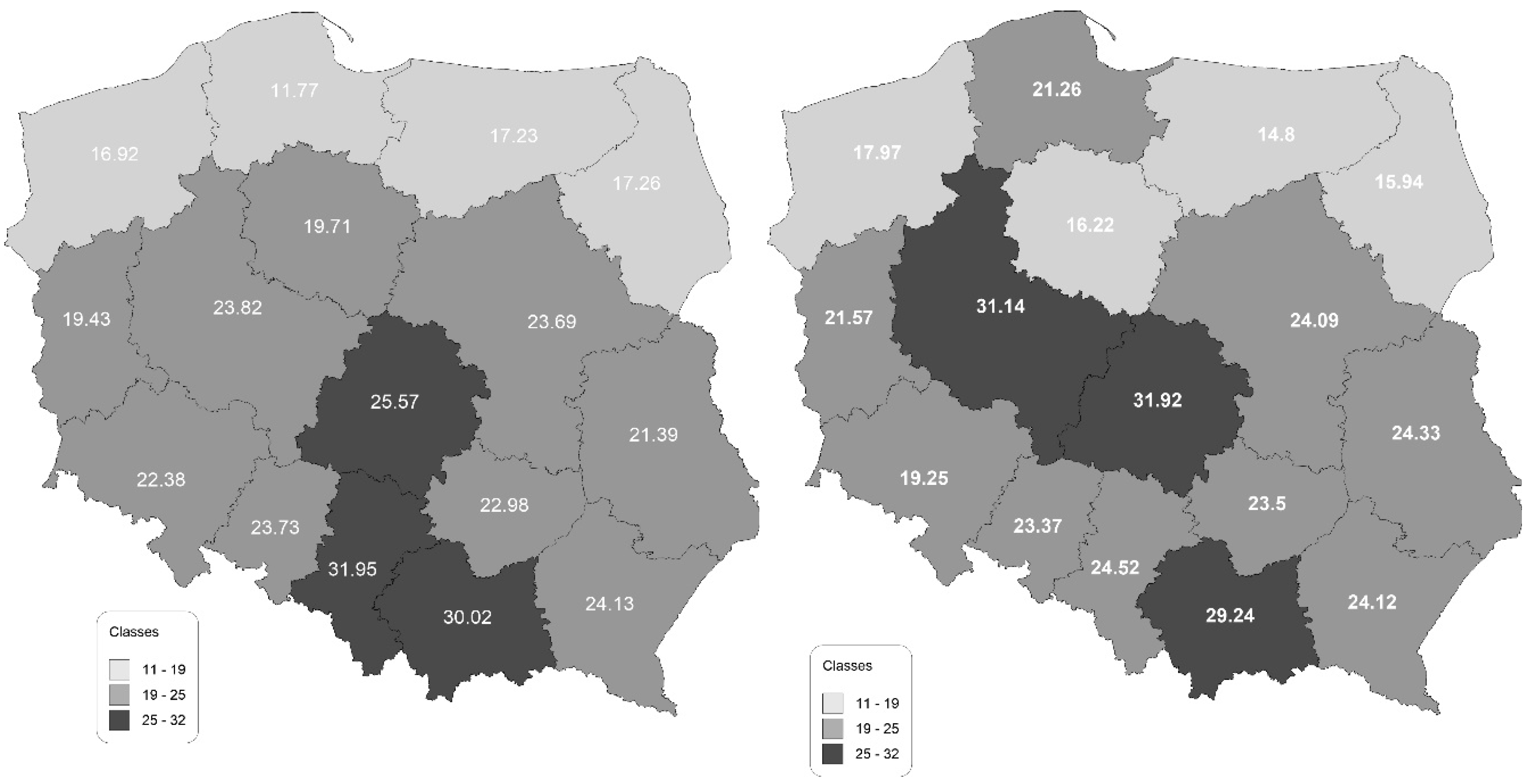
Region	Rural District			Cities
	Mean	Min	Max	Mean	Min	Max
dolnośląskie	19.25	1.64	216.75	22.38	2.44	246.35
kujawsko-pomorskie	16.22	1.37	123.03	19.71	2.23	182.16
lubelskie	24.33	5.23	147.27	21.39	2.2	290.45
lubuskie	21.57	5.10	131.10	19.43	2.37	139.78
łódzkie	31.92	5.09	292.00	25.57	2.6	244.8
małopolskie	29.24	4.57	190.83	30.02	3.67	244.8
mazowieckie	24.09	1.39	376.13	23.69	3.35	176.21
opolskie	23.37	1.33	254.27	23.73	2.5	238
podkarpackie	24.12	2.47	222.85	24.13	4.2	190
podlaskie	15.94	1.47	172.44	17.26	0.58	152.21
pomorskie	21.26	0.81	182.18	11.77	0.62	103.89
śląskie	24.52	5.60	169.03	31.95	4.4	342.57
świętokrzyskie	23.50	2.46	233.87	22.98	2.14	281.66
warmińsko-mazurskie	14.80	2.14	90.94	17.23	2.13	131.76
wielkopolskie	31.14	4.30	206.20	23.82	1.7	212.96
zachodniopomorskie	17.97	3.20	118.91	16.92	0.9	143.09
country average	22.70	3.01	195.49	22.00	2.38	207.54

in Appendix A). Furthermore, a typical phenomenon in Poland, as well as in other countries of Central and Eastern Europe, is that rural districts may pollute even more than big cities, as advocated by Figure A1, where mean levels of PM_2.5 concentration in Poland are given on regional level for both cities and rural areas. For example, in Greater Poland (Wielkopolskie voivodship), a leading agricultural region in Poland, the annual average emission in rural areas is 31% higher than in cities.

Plant cover plays an essential role in the struggle against pollution by absorbing airborne toxins. According to calculations prepared by the Centre for Ecology and Hydrology (CEH) and published on the UK statistical office’s website, plants helped save the lives of around 1900 UK residents in 2015 [9]. Winds transport smog clouds to non-urban areas and their degree of absorption is dependent on plant cover. Considering the above, the role of the non-urban area is ambivalent. On the one hand, they determine the absorption of air pollutants and are a refuge for the natural environment. On the other hand, agriculture is developing in these areas, which, as mentioned above, is an important source of particulates emission.

Taking into account the above considerations, we determined that there is still a need to examine the adequacy of policy instruments by comparing inputs and effects. Since the end of the 1990s, cost-benefit analyses have gradually become more routine and their development is very much needed in the policy-making process [10]. In this context, the question arises as to what extent the increasing expenditures on individual measures related to environmental protection are accompanied by adequate effects on the improvement of the environment quality.

There is a relatively large body of literature on the environmental quality and public policy so one can distinguish different streams of research regarding these issues (cf. literature review section). Our study is a part of the research trend on the relationship between public expenditure and its effects on natural environment. This type of research is, however, still underdeveloped and provides ambiguous results. In particular, there is a lack of research that would attempt to address the role of structural factors affecting the effectiveness and/or efficiency of environmental expenditures. This paper tries to fill this gap by the inclusion of agriculture share as a factor influencing policy efficiency.

The novelty of our approach might be manifested in several aspects:

• We run a comprehensive comparative assessment of the financial efficiency of different national schemes for environment protection in the panel of 25 European Union countries (2004–2016);
• We use an index of PM_2.5 pressure on the environment (calculated as PM_2.5 emissions per hectare of non-urban areas). This is used instead of a commonly used simple emission indicator as we believe that the non-urban areas matter when struggling with PM_2.5 pollution due to their natural absorbent capacity;
• We test the hypothesis that agriculture’s share in non-urban areas is a significant factor which contributes to PM_2.5 emission and handicaps anti-smog policy;
• We use a novel econometric approach in this field i.e., seminal within–between specification of Bell and Jones [11] with multilevel random effects that may identify potential sources of environmental policy inefficiency.

The seminal “within–between” estimation carried out in the study explores two aspects of the policy impact on PM_2.5: Firstly, it gives an insight on how an increase in the environment expenditures translates into a downturn of pollution. This is a dynamic aspect of the problem reflected by the “within” component and we should indeed expect a negative coefficient to prove the efficiency. Secondly, we address the question whether in those countries which spend more on the environment, the pollution is relatively lower. In this case a negative estimator also would confirm the efficiency of PM_2.5 pollution management. So, the negative signs in both above-mentioned cases indicate ex ante efficient management while the negative “within” and positive “between” coefficient suggests that the efficient policy has been implemented ex post as a response to high pollution. The positive coefficients prove that neither ex ante, nor ex post policy is efficient. Why do we use the term “efficiency” instead of “effectiveness”? It should be noticed that we deal with relative changes and cross-sectional differences of PM_2.5 caused by the national expenditures, disregarding the absolute assessment of PM_2.5 concentration in terms of the legally permitted exceedances. So, the overall effectiveness is out of the question in this perspective.

The rest of the paper is organized as follows. In the next section we review literature on the determinants of air pollution and the interaction between its level and public policy. We then provide the methodology for our analysis together with data descriptions. The next section then presents results and a discussion while the last part concludes.

2. Literature Review

The severe effects of air pollution have prompted many authors to study the determinants of air quality and the effectiveness or efficiency of public policies to reduce emissions of particulates and greenhouse gases. In studies using econometric methods referring to European countries, air quality is often assessed through the prism of GHG emissions (i.e., ozone and carbon, nitrogen and sulphur oxides) or by means of air quality indices. De Almeida et al. [12] analyzed air quality in individual regions of Portugal and concluded that the main determinants influencing air quality included forest fires and the number of manufacturing industries per km². Rafaj et al. [13] studied the drivers of GHG emissions in the years 1960–2010. The study was limited to European countries, which were divided into Eastern and Western ones. The relative influence of particular determinants on emission levels differed depending on the pollutant; however, the authors indicate that the decrease in SO₂ emissions in Western countries was mainly due to reduced energy intensity and improved fuel mix. In the 1990s, GHG emissions in Eastern Europe grew despite the improvement in fuel quality, which was due to an increase in energy-intensive industries.

The drivers of PM_2.5 emissions were studied mostly by Chinese researchers. Using panel regression models for the Chinese provinces, Xu and Lin [14] identified economic growth as a main determinant of emission levels. The relative role of the other analyzed factors (level of urbanization, private cars, energy efficiency, R&D investment, coal consumption) was different for each region. Adequate policies should therefore be regionally flexible. Luo et al. [15] claimed that the key determinant of particulate emissions is the share of the secondary sector in the economy, even before the level of GDP per capita. Furthermore, the quality of the environment is also influenced by urbanization, population density, energy intensity, and the proportion of the tertiary sector (the impact of the latter variable was negative). With regards to the relationship between GDP per capita and PM_2.5 emissions, there is the so-called environmental Kuznets curve (EKC). The EKC states that particulate matter emissions increase proportionately with income until a certain level of economic development is achieved. Once this level of development is reached, emissions begin to decrease proportionately with additional increases in income [16]. This theoretical model explains why studies on the relationship between GDP and particulate matter emissions in developing countries show a positive relationship between these variables [17,18] and a negative relationship in developed countries [19].

The above studies have focused on analyzing direct determinants of pollutant emissions; however, political and institutional factors also influence the quality of the environment and the efficiency of environmental policy. Crepaz [20] pointed out that the political system described as corporatism (e.g., in Scandinavian countries and Germany) affects the reduction of GHG emissions in comparison to the pluralist system. In European countries, public spending contributed to the reduction of greenhouse gas emissions, whereas in the Middle East the effect was insignificant or even positive [21]. Similar conclusions were reached by Gholipour and Farzanegan [22]. Using countries in North Africa and the Middle East as an example, they proved that environmental funds alone do not have a significant impact on the quality of the environment. Adequate governance quality is still needed, and only then do the funds begin to significantly reduce emissions. Using the quantile panel regression for G20 countries, Wang et al. [23] have shown that the level of democratization and globalization was positively correlated with particulate matter emissions (PM_2.5). The first of these factors has a particularly large impact in countries with high emissions, while the second factor impacts countries with very low or high levels of emissions.

There are four research trends studying the relationship between environmental policy and air quality. The first group includes studies aimed at assessing the impact of specific policy mechanisms on environmental quality. Erjavec et al. [24] stated that despite the fact that many agricultural policy instruments were not directly aimed at reducing GHG emissions or adaptation to climate change, instruments with a large budget addressed to many recipients contributed to the improvement of the natural environment. Finn et al. [25] examined ex-post the impact of agri–environmental schemes (AEs) on the achievement of environmental objectives. Significant differences in the achieved environmental performance among the examined regions were found, and at the same time there was no correlation between the efficiency of AEs and the priority level of a given policy goal. Neufeldt and Schäfer [26] analyzed how the introduction of various environmental policy instruments would reduce GHG emissions from agriculture. The authors pointed out that the choice of one mechanism is tedious, because e.g., an emission cap means low costs for farmers, while an emission tax is cheaper on a macro scale. Morley [27] used a panel of EU countries and Norway to prove that there is a statistically significant negative correlation between the level of environmental taxes and the level of GHG emissions. These taxes have therefore proved to be effective. Dholakia et al. [28] indicated that the assessment of the effectiveness of air quality policy is also influenced by the quality measure used. Policies in India, for example, have contributed to a significant reduction in CO₂ emissions, but have only a limited impact on particulate matter emissions. Reducing the latter would require more rigorous action.

The second group of studies involves papers examining the environmental impact of total public expenditure, sometimes expressed in relation to GDP. Using the example of 12 European countries in 1995–2008, López and Palacios [29] proved that fiscal spending played a significant role in reducing sulphur oxide and ozone emissions. However, such an effect was not recorded for nitrogen oxide. In other studies, López et al. [30] examined both the direct impact of budgetary expenditure on air and water quality and the indirect effect through the channel of GDP growth. They found that an increase in expenditure without changing its structure towards the financing of public goods did not contribute to the reduction of pollution. On the example of China, Feng and Fang [31] claimed that to record the positive impact of public spending on the quality of the environment at the local scale, it was necessary to achieve an appropriate level of economic development. Halkos and Paizanos [32,33] studied the impact of government spending on GHG emissions on panels of 77 and 94 countries, respectively. They found that while a higher share of public spending in GDP was conducive to reducing emissions of sulphur and nitrogen oxides, there was no such effect on carbon dioxide. Moreover, in low-income countries, the impact of government spending on reducing emissions is strong, but in richer countries there can even be a positive correlation between rising spending and emissions. In general, the indirect effect of public spending is more important and strengthens with GDP growth and the level of democratization.

The aim of the third research area is to determine the impact of air quality on the level of public expenditure, in particular on environmental or health protection. This is therefore the opposite approach to the one adopted in our study. This type of research is carried out primarily for developing countries. Yahaya et al. [34] found on a panel of 125 developing countries that air quality significantly determined the health expenditure per capita in these countries, with a particularly strong impact on carbon dioxide. Yang and Zhang [35] found that exposure to PM_2.5 had a significant impact on household health expenditure, even after socioeconomic characteristics and country locations were included in the model. Interestingly, Ma et al. [36] reported no positive correlation between air pollution (as measured by the air quality index) and the increase in public investment for environmental protection within the Chinese provinces. Moreover, the increase in emissions had even been accompanied by a decrease in public spending.

This article falls into the fourth research stream, which concerns the impact of environmental expenditure on air quality expressed through the prism of various indicators. He et al. [37] studied the impact of environmental expenditures on air quality (air quality index) on a panel of seven Chinese cities. In panel analyses, there was no correlation between the increase in expenditures and improvement in air quality. In single models, such a correlation was noted in four cities if the share of environmental expenditures in the total spending was indeed significant. The direct impact of funds on air quality was also not recorded in the case of North Africa and the Middle East [22]. Ouyang et al. [19] found that the impact of the funds on pollutant emissions (PM_2.5) in the OECD countries was even positive, but this was due to the fact that in developed countries there was often both a decrease in emissions and a decrease in expenditure on air quality protection. Thus, in the econometric modelling, a positive sign in the regression coefficient was obtained. On the other hand, Bostan et al. [38] came to different conclusions, when examining the impact of public expenditure and investments on the level of pollution (PM_2.5 and sulphur, nitrogen and carbon oxides). They found that environmental protection expenditure by general government had a significant impact on the decrease in emissions for each type of air pollution taken into account.

Due to the potential serious health consequences for the population, in this article we focused on the impact of public financial spending on the level of particulate matter emissions (PM_2.5). Unlike some authors who analyzed the environmental impact of total public spending [29,32,33], this study specifically analysed the impact of environmental national spending (source: Eurostat). In doing so, we followed the conclusion of López et al. [30], who stated that the key to achieving environmental objectives is a structure of public spending that shifts towards financing public and social goods. At the same time, instead of analyzing the impact of funds on total air protection against other socioeconomic variables [19], we limited ourselves to financial inputs. However, following Bostan et al. [38], we presented them in a more detailed breakdown in order to assess the efficiency of particular types of expenditures.

3. Material and Methods

3.1. Variables Selection

For the long-term assessment of the environmental policy in EU-25 countries we primarily use data from Eurostat and Faostat, depicted in

Table 1. Descriptive statistics of variables.

Variable	Mean	Stand. Dev.	Min	Max
PM2.5 in kg per ha of non-urban areas (1)	6.62	9.29	0.46	103.20
Pollution abatement in EUR per ha of non-urban areas (2)	75.91	212.25	0.00	1209.08
Protection of biodiversity in EUR per ha of non-urban areas (3)	91.63	230.17	0.00	1266.53
R&D Environmental protection in EUR per ha of non-urban areas (4)	10.85	19.47	0.00	176.34
Environmental protection n.e.c. in EUR per ha of non-urban areas (5)	35.86	54.77	0.00	451.14
Share of UAA in non-urban areas CLASS 1	0.96	0.12	0.76	1.17
Share of UAA in non-urban areas CLASS 2	0.53	0.12	0.28	0.75
Share of UAA in non-urban areas CLASS 3	0.15	0.07	0.07	0.28

Note: UAA stands for utilized agricultural area, n.e.c—non-elsewhere classified.

and

Table 2. Mean values of variables for panel of 25 EU countries.

Country	1	2	3	4	5	Average Share of UAA in Non-Urban Areas
Malta	44.33	68.75	1124.44	16.73	174.74	0.81
Belgium	12.83	236.74	70.76	16.13	176.73	0.58
Luxembourg	10.42	186.30	179.38	3.48	63.13	0.73
Netherlands	10.27	1036.56	409.02	72.86	85.15	1.10 *
Italy	7.46	34.99	128.17	12.81	25.19	0.59
Slovenia	6.89	8.33	24.01	4.71	16.97	0.33
United Kingdom	6.64	16.59	30.73	37.55	103.75	0.97
Czech Republic	6.39	10.89	48.86	3.40	1.80	0.60
Slovakia	6.33	3.85	6.25	1.54	11.62	0.41
Portugal	6.20	2.44	22.90	3.75	15.86	0.43
Denmark	5.60	35.07	85.35	32.60	66.16	0.62
Hungary	5.27	4.52	3.67	0.14	6.55	0.60
Poland	5.27	4.92	2.23	3.10	11.50	0.51
Latvia	3.75	1.87	1.28	0.05	2.05	0.34
Germany	3.73	98.66	33.54	28.68	35.17	0.53
Greece	3.66	32.92	0.07	0.00	3.18	0.59
Spain	3.65	14.80	36.46	10.20	14.41	0.71
France	3.54	22.11	22.09	7.15	27.84	0.49
Ireland	2.82	13.77	42.57	1.60	9.39	0.64
Estonia	2.81	0	4.47	2.39	6.21	0.23
Austria	2.60	59.57	7.12	9.11	21.64	0.36
Cyprus	2.51	3.54	0.45	0.00	0.00	0.18
Lithuania	1.27	0.13	1.97	0.37	5.40	0.51
Finland	0.73	3.66	1.92	1.87	4.00	0.07
Sweden	0.58	0.40	3.17	1.05	8.05	0.08

Note: c.f Table 1 for variables names; * shares above 1 indicates that UAA are located in urban areas to some extent.

(the full database used for analysis can be found via link in Supplementary Materials). We use the complete matrix of public expenditures on environmental policy. We recall that the aim is to estimate the efficiency of a comprehensive range of environmental schemes which directly or indirectly may affect the pressure of PM_2.5 on the natural environment understood as non-urban-areas (i.e., total country area minus urban area). PM_2.5 in kg per ha of non-urban areas stands for the dependent variable, and the following selection of national expenditures in real prices (2004 = 100, deflated by HICP) for the explanatory variables:

• Pollution abatement in EUR per ha of non-urban areas (direct impact on PM_2.5) which comprises measures and activities aimed at (a) the reduction of emissions into the ambient air, (b) ambient concentrations of air pollutants, and (c) measures and activities aimed at the control of emissions of GHG’s and other gases that adversely affect the stratospheric ozone layer. Pollution abatement refers to technology applied or measures taken to reduce pollution and/or its impacts on the environment. The most commonly used technologies are scrubbers, noise mufflers, filters, incinerators, heating devices, wastewater treatment facilities, and composting waste.
• Protection of biodiversity in EUR per ha of non-urban areas (indirect impact on PM_2.5) which comprises the protection of species, landscapes, and habitats (including mainly forests); the rehabilitation of species populations and landscapes; the restoration and cleaning of water bodies; and the measurement, control, and other in-laboratory activities.
• R&D on environmental protection in EUR per ha of non-urban areas (indirect impact on PM_2.5) which covers research on the protection of ambient air, climate, soil, and water. R&D also studies the abatement of noise and vibrations, the protection of species and habitats, and the protection against radiation and waste management.
• Environmental protection n.e.c. (non-elsewhere classified) in EUR per ha of non-urban areas (indirect impact on PM_2.5) which includes general administration of the environment, education, training and information, and activities leading to indivisible expenditure.

The first scheme is directly linked to the PM_2.5 emission, whereas the rest of the expenditures may presumably affect PM_2.5 pressure on the environment. In our research we also controlled for unobserved individual effects (fixed and random) of the selected countries while focusing on the share of utilized agricultural area (UAA) in non-urban areas as a proxy for the natural environment. The latter aims to test the hypothesis raised in the introduction that agriculture might affect environmental policy efficiency. Our approach to this problem is presented in the next section. In the first step we attempted to identify “typical” and “outstanding” shares of UAA in the panel of selected countries. UAA share distribution for EU-25 is close to the Gaussian (normal) distribution. For that reason, to distinguish the “typical” and “outstanding” classes of UAA share we used the mean $(\overline{z)}$ +/− and the standard deviation $(s_z)$. Hence, we obtained three classes, where the second covers about 70% observations with the mean 0.53 (which is close to the normal distribution assumption), the first and third comprises observations (country c in year t) with noticeable high and low UAA shares (cf. Table 1):

$$\mathrm{UAA}\mathrm{class}1:\overline{z}+s_z\le z_i$$

$$\mathrm{UAA}\mathrm{class}2:\overline{z}-s_z\le z_i<\overline{z}+s_z$$

$$\mathrm{UAA}\mathrm{class}3:z_i<\overline{z}-s_z$$

Descriptive statistics show a significant diversity of the studied panel, both in terms of environmental pressure understood as PM_2.5 per hectare of non-urban areas, as well as individual types of expenditures on environmental protection. The average particulate matter emission was 6.62 kg/ha; however, in the Benelux countries emissions were above 10 kg/ha on average, and in Sweden and Finland the average was below 1 kg/ha. Among the analysed expenditures, the largest funds were allocated for biodiversity protection. However, in some countries (Italy, Luxembourg, Malta, the Netherlands) the inputs exceeded EUR 100/ha, while in Greece, Cyprus, Finland, Latvia, Lithuania and Latvia they were below EUR 2/ha. Relatively less was spent on research and development related to environmental protection. In general, it can be stated that in countries with higher particulate matter emissions, higher total expenditure on environmental protection was also recorded (the value of the correlation coefficient was 0.74).

The first class of UAA share in non-urban areas comprises three countries: The Netherlands, United Kingdom, and Malta. These are highly urbanised countries so their non-urban areas almost entirely consist of agricultural areas. At the other extreme are Estonia, Cyprus, Finland, and Sweden. With the exception of Cyprus, these are states with low population density and vast non-urban areas covered by forests. Therefore, the share of UAA is rather low and does not exceed 28%. The rest of the countries have a moderate share of UAA in non-urban areas.

It is also worth discussing the compound annual rate of change depicted in

Table 3. Compound annual rates of change for PM_2.5 and environmental expenditures in EU25 over 2004–2016 (%).

	Compound Annual Rate of Change of PM2.5 Per Ha of Non-Urban Area	Compound Annual Rate of Change of Pollution Expenditures	Compound Annual Rate of Change of Total Environmental Expenditures
Malta	−12.35	−17.87	1.65
Belgium	−3.13	6.91	1.22
Luxembourg	−4.16	4.06	1.88
Netherlands	−5.59	−1.59	−0.29
Italy	0.57	−2.93	0.50
Slovenia	0.44	9.57	−2.57
UK	−1.51	−8.59	−0.10
Czech Rep.	−1.71	−6.29	0.55
Slovakia	−0.66	7.08	3.26
Portugal	−2.42	20.99	0.55
Denmark	−1.54	−3.61	−1.29
Hungary	1.92	17.45	−2.44
Poland	−1.24	14.12	1.70
Latvia	−3.64	7.74	3.36
Germany	−2.84	9.32	1.97
Greece	−6.34	17.20	7.23
Spain	−1.70	−11.84	−0.39
France	−4.08	4.84	1.91
Ireland	−3.23	−4.55	−4.56
Estonia	−5.86	−2.65	1.98
Austria	−2.40	−0.79	−0.65
Cyprus	−4.69	14.97	0.37
Lithuania	−1.96	−1.33	4.48
Finland	−3.08	3.98	−0.90
Sweden	−3.11	5.52	1.65

Note: this variable is independent of the base year chosen and gives the same result for any of them, using the formula RCH_A_C = (Y_t/Y_t0) ^1/t–t0 − 1, where t₀ = the earliest year; t = the most recent year; Y_t0 = indicator value in the earliest year; and Y_t = indicator value in the most recent year. In economics, this variable is known as the compound annual growth rate and measures e.g. return on an investment over a defined period of time.

and Figure 1. We can see how annual average changes in PM_2.5 pressure correspond with the dynamics of environmental policy expenditures. In most countries, we observe a decreasing trend of PM_2.5 pressure on non-urban areas. Italy, Slovenia, and Hungary were the only countries where emissions were, on average, slightly increasing. Emissions were decreasing at the fastest pace in Malta, followed by Estonia and Greece. In all of these countries the average annual growth in environmental expenditures can be observed; however, the expenditures directly linked to air pollution were increasing only in Greece. Based on Table 3, we can see substantial differences when it comes to expenditure patterns. In 11 countries, the downward trend in pollution abatement expenditures can be observed, while in 14 countries spending increased. In Portugal the annual rate of change was 20.99%, while in Malta it was −17.87%. However, a decreasing (negative) average rate of change in total expenditure was only recorded in nine countries and in Slovenia this effect was the strongest with Slovenia being the lowest.

3.2. Economic Strategy

We use a multi-level panel model with the seminal within–between specification. Typical panel regressions explore time and cross-sectional dimension at the same time. We introduce simultaneously UAA classes as a third level of the analysis. Hence, our model attempts to estimate comparative effects of different policy schemes on PM_2.5 while controlling the following heterogeneity and endogeneity source that may possibly bias the results:

• Observed fixed cross-sectional effect to address potential reverse causality of PM_2.5 influence on the expenditures,
• Unobserved time-invariant heterogeneity of countries (so called random effect or intraclass variance for the countries),
• Unobserved time-invariant heterogeneity of UAA shares in non-urban areas (so called random effect or intraclass variance for different UAA share),
• Random parts of regression coefficients which reflect changes of policy efficiency accordingly to the share of UAA.

A prominent advantage of using panel data is that they contain information about the heterogeneity of the phenomenon in which we are interested, both in time and space (and here we address two space levels). However, most panel data methods do not allow us to separately model the consequences of changes of that phenomenon over time or the effects of its heterogeneity in space. The fixed effect (FE) models allow to investigate only the “within” effect so they can be useful to answer what is the average response of dependent variable if occasion-level time-variant variable changes by unit. The higher-level (between) variance is modelled out so we cannot say anything about the effect of explanatory variables on the differences in dependent variable between entities. Random effects (RE) models deal with these problems only to some extent. The calculated betas encompass both between and within effect but if we assume that these effects are different (what is very likely in social science problems) then RE model does not solve the problem of different impact of variable in time and space dimension [11].

To compensate for this, a novel approach called “the seminal within–between specification” advocated recently by Bell and Jones [11] solves this problem as it allows to estimate the “within” (in-time) and “between” (in-space) effect separately We employ this specification with the additional space level (UAA share) which could also potentially cause random effects. However, we apply a three-steps modelling procedure. In the first step we estimated a so called “base model”. As standard errors in our estimation may be biased by heteroscedasticity and autocorrelation issues we use robust standard errors proposed by Arellano [39]. In the second step we add the level of the UAA class as an additional grouping variable, and finally we adopt the assumption that the UAA class may also influence the regression coefficients. We decide whether the next step is justified on the basis of loglikelihood criterion which should indicate a significant improvement of the goodness of fit. These steps are depicted in the following models and estimations results are presented in

Table 4. Multilevel panel models results.

Explanatory Variables	1			2			3
	Coeff.	S.E.		Coeff.	S.E.		Coeff.	S.E.
FIXED PART
Intercept	3.1170	0.4310	***	5.1786	2.1590	***	4.1408	0.6851	***
Betw_pollution abatement	−0.0036	0.0027		0.0073	0.0040	*	0.0069	0.0059
With_polution abatement	−0.0089	0.0042	**	−0.0061	0.0030	**	−0.0638	0.0366	**
Betw_protection of biodiversity	0.0297	0.0020	***	0.0365	0.0043	***	0.0248	0.0019	***
With_protection of biodiversity	−0.0580	0.0062	***	−0.0321	0.0049	***	−0.0329	0.0051	***
Betw_R&D environmental prot.	−0.0819	0.0368	***	−0.1205	0.0490	***	−0.0740	0.0319	***
With_R&D environmental prot.	−0.0779	0.0222	***	−0.0495	0.0164	***	−0.0425	0.0201	***
Betw_environmental prot. n.e.c.	0.0542	0.0102	***	0.0299	0.0117	***	0.0512	0.0091	***
With_environmental prot. n.e.c	−0.0058	0.0088		−0.0081	0.0065		−0.0093	0.0066
RANDOM PART
Intraclass variances and covariances	Var/Cov	S.E.		Var/Cov	S.E.		Var/Cov	S.E.
Level of UAA share
Intercept variance	−	−		54.3092	20.9133		4.5135	2.2437
Betw_pollution abat. variance	−	−		−	−		0.0003	0.0001
With_pollution abat. variance	−	−		−	−		0.0157	0.0070
Intercept/With_poll. covariance	−	−		−	−		−0.2759	0.1187
Intercept/Betw_poll. covariance	−	−		−	−		0.4290	0.0176
Betw_poll/With_poll. covariance	−	−		−	−		−0.0023	0.0010
Level of country
Intercept variance	1.6473	0.7762		1.2900	0.6907		1.2799	0.6797
Residual variance eij	14.0736	1.1491		7.5140	0.6187		7.5850	0.6301
No obs.	325			325			325
ICC (intraclass correlation coeff.)	0.11			0.88			0.43
−2*loglikelihood:	1795.836			1650.3622			1640.2430
pseudo-R2	0.83 (within 0.81)			0.91 (within 0.27)			0.91 (within 0.85)

Source: own calculation using MLwiN 2.36; *** p < 0.001, ** p < 0.05, * p < 0.1.

:

First “base” model (typical panel regression with seminal “within–between” specification):

$$y_{c,t}={\propto }_{c,t}+\beta \left(x_{c,t}-{\overline{x}}_c\right)+\gamma {\overline{x}}_c\mathrm{st}.{\propto }_{c,t}={\propto }_0+{\delta }_{0c}+e_{a,c,t}$$

(1)

Second model with additional grouping variable (UAA class):

$$y_{a,c,t}={\propto }_{a,c,t}+{\beta }_a\left(x_{c,t}-{\overline{x}}_c\right)+{\gamma }_a{\overline{x}}_c\mathrm{st}.{\propto }_{a,c,t}={\propto }_0+{\delta }_{0c}+{\mu }_{0a}+e_{a,c,t}$$

(2)

Third model with the assumption of random coefficients for UAA classes. We present the estimated equation as well as the matrix of variances and covariance that is possible to obtain in this approach:

$$y_{a,c,t}={\propto }_{a,c,t}+{\beta }_a\left(x_{c,t}-{\overline{x}}_c\right)+{\gamma }_a{\overline{x}}_c\mathrm{st}.{\propto }_{a,c,t}={\propto }_0+{\delta }_{0c}+{\mu }_{0a}+e_{a,c,t}$$

(3)

$${\beta }_a={\beta }_1+{\mu }_{1a}$$

$${\gamma }_a={\gamma }_2+{\mu }_{2a}$$

$$\left[\begin{array}{c}{\mu }_{0a}\\ {\mu }_{1a}\\ {\mu }_{2a}\end{array}\right]~N\left(0,{\Omega }_u\right):{\Omega }_{\mu }=\left[\begin{array}{ccc}{\sigma }_{{\mu }_0}^2& & \\ {\sigma }_{{\mu }_1{\mu }_0}& {\sigma }_{{\mu }_1}^2& \\ {\sigma }_{{\mu }_2{\mu }_0}& {\sigma }_{{\mu }_2{\mu }_1}& {\sigma }_{{\mu }_2}^2\end{array}\right]$$

where $x_{c,t}$ is a set of time-variant variables (the expenditures) so called “within-”, ${\overline{x}}_c$ consists of x_c,t means called “between-” calculated for each country c (which by definition are time-invariant). The intercept (free term) ${\propto }_{a,c,t}$ consists of four parts: Fixed term ${\propto }_0,$ random effects (estimated as variances) ${\delta }_{0c}$ and ${\mu }_{0a}$, respectively for the country level (c) and UAA class (a) that reflect the unobserved heterogeneity of these levels, and $e_{a,c,t}$ as an idiosyncratic disturbance for each observation. The parameter β_a reflects the within effect (changes in time), while ${\gamma }_a$ captures the between effect, which can be interpreted as the impact of a unitary difference in x_c,t among EU-25 countries on the dependent variable (reverse causality may also happen in this case). In addition, we assume that the UAA class may also influence the regression coefficients β_a and ${\gamma }_a$, so they also consists of a fixed part (${\beta }_1$ and ${\gamma }_2$) and a random part (${\mu }_{1a}$, ${\mu }_{2a}$), estimated as variances; ${\Omega }_{\mu }$ stands for the matrix of variances and covariances attributed to the UAA class (${\sigma }_{\mu }^2$ variances; ${\sigma }_{\mu }$ covariances).

The assumption adopted above that the UAA class may influence the regression coefficients implicates different policy efficiency, accordingly to the UAA class. This is depicted in Figure 2, where we can see three regression lines with a different slope.

The regression line for CLASS 3 intersects the abscissa axis in 20 € which means a growth of pollution abatement expenditures is required to achieve zero-emission. For the second and third CLASS, the intersection points are respectively higher which may be interpreted as lower efficiency of the anti-smog policy.

The model was calculated using the maximum likelihood (ML) method, which has less restrictive assumptions than OLS, defined in the MLwiN software used for this study as IGLS (Iterative Generalised Least Squares). In this approach, the R² statistic is not calculated, and the fit of the model can be evaluated on a relative basis by comparing the statistic “–2 log likelihood”. The decision on whether the introduction of a random intercept and random coefficients into the model is statistically significant is taken on the basis of a likelihood ratio test (LRT), as mentioned. We perform this on each occasion by calculating the difference between the “–2 log likelihood” statistics for the model with and without a random term [40]. We also computed the intraclass correlation coefficient (ICC) based on the variance of the intercepts and the remaining residual variance (as a relation of intraclass variance to total variance). This coefficient shows what part of the unobserved heterogeneity of PM_2.5 can be attributed to grouping variables used in a model [40].

3.3. Robusteness

The within–between specification can be treated as a variant of a random effects model, where explanatory variables are divided into their time and varying cross-country parts. The seminal within–between model makes it possible to solve the endogeneity problems found in RE modelling. According to Wooldrige [41], the RE model is consistent only if the within and between variances are equal. Otherwise, the estimation is biased since the unaccounted variance will be absorbed by the unit-specific error and will be correlated with the independent variables, violating the assumptions of the RE model. This problem would be inevitable in our dataset. It is also very likely that a high emission of PM_2.5 may implicate the higher ex post expenditures. This type of endogeneity problem has been successfully solved using the within–between approach in many empirical studies in the field of economics [42,43] therefore, we also apply this approach in our study. We also tested for the presence of autocorrelation using the Born and Breitung test and it was proved that autocorrelation is not present.

4. Results and Discussion

All three models are well fitted with pseudo-R² from 0.83 in the base model to 0.91 in the third model. If we exclude the unobserved, intraclass heterogeneity (so-called “between”) that is attributed to the countries and UAA class, the “within-R2” equals, respectively, 0.81, 0.27, and 0.85. This indicates that the third model has the best goodness of fit, that is confirmed by the lowest loglikelihood score. In the second model, the between variance grew rapidly since the UAA random effects has been included to the intercept, but the coefficients are still biased. The variables are all significant except within_environmental protection n.e.c and between_pollution abatement in the first and third model (cf. Table 4). We recall that “between” variables coefficients undergo cross-sectional interpretation, whereas “within” variables reflect the effects of changes in time. Thus, we have expected minus signs for all within-expenditures and this is the case here. Therefore, we can say that the influence of the EU-25 environmental policy on reducing PM_2.5 emission has been proved in that a growth of expenditures causes a significant decrease in PM_2.5. This is similar to the conclusion from Bostan et al. [38], who also found a significant effect of public expenditures on the decrease of pollution. Also similar observation was found by Xie and Wang [44]—according to their analysis government financial input has an obvious influence on the improvement of air quality, especially when they considered inhalable particulate matter (PM_2.5, PM₁₀), sulfur dioxide (SO₂), and nitrogen dioxide (NO₂) in the year 2006 to 2015 in China. Based on our results, we can conclude that the EU environment policy is an efficient tool to struggle with PM_2.5. These findings are also in line with the notion of López et al. [30], who stated that achieving environmental goals requires the shift into financing public goods since a high quality of environment can be considered as one of the goals.

However, when it comes to the specific “between” variables, there are positive signs for all of them except between R&D environmental protection. This means that a higher average level of expenditure corresponds to a higher PM_2.5 emission. According to the previous assumption, we can conclude that a majority of environmental schemes in Europe have been designed ex post in response to the unsatisfactory emission level. In this sense only R&D expenditure is efficient ex ante since both “between” and “within” measures have obtained minus signs. Hence, the seminal within–-between specification might be an interesting tool to distinguish ex post and ex ante policy efficiency. Complementary analyses made by Fernandez et al. [45] suggest that innovation and R&D expenditure have had a positive effect on reducing CO₂ emissions for the European Union (15), the United States and China between 1990 and 2013. Similar conclusions were also found for Japan [46].

The next point of analysis is a comparative efficiency of specific policy schemes. Taking the third model under consideration, we can see that the “within-pollution abatement” has the strongest impact on PM_2.5 with the fixed coefficient equal to −0.064. This means that an increase of the expenditure by 1€ translates into a fall of PM_2.5 emission per ha by 0.06 kg. It is worth noting that this coefficient changes considerably when comparing the first and second model. This fact confirms that the share of UAA in non-urban areas really matters and this includes the random variance of UAA class. On the other hand, the lowest effect is brought by the protection of biodiversity, with a −0.033 reduction per 1€ of spent funds. This gives a clear suggestion of which environmental policy direction is most and least efficient, and what should be improved. One may note that in a “base” model the marginal effect of “within-pollution abatement” expenditures on the dependent variable is weaker than R&D or the protection of biodiversity funds. However, as we mentioned above, this effect is underestimated due to the bias of UAA class heterogeneity which has not been fully controlled in either the first or the second model.

We then move the discussion to the part of the model that gives valuable insight into the meaning of level variables (i.e., country and UAA class). The levels gather unobserved variance (heterogeneity), and the intercept variance for UAA level is the most important. All random effects turned out to be significant but only a random coefficient for the pollution abatement (both within- and between-) has improved the model. The intercept variance for UAA class is 4.51, and there are 1.28 and 7.58 for the country level and the residual, respectively. This gives ICC = 0.43 in total, meaning that the unobserved heterogeneity attributed to the country and UAA class is very high, with a notifiable supremacy of the latter. Thus, we confirm the hypothesis that the outstanding UAA share in non-urban areas plays an important role in PM_2.5 emission as it moves up (or down) the expenditures regression line. Moreover, it also changes the coefficient for “within-pollution abatement”, revealed by the significant random variance of 0.0157 (cf. Table 4, random part for UAA share). Hence, a pre-eminent share of UAA in non-urban areas makes the environmental policy less efficient (as depicted in Figure 2), and a lower-than-average share produces the opposite. When it comes to the covariances, its signs are in line with expectations: A higher coefficient for the “within-pollution” expenditures (i.e., more efficient policy), and lower constant of PM_2.5 emission (cf. cov. = −0.2759, Table 4) assuming that environmental expenditures equal zero.

To conclude, the random part of the model depicting the impact of agriculture on PM_2.5 emission and policy efficiency turned out to be the most meaningful for the answer to the question raised in the title. We can literally see there how agriculture make the difference as it hampers the effect of all environmental expenditure, especially those which concern pollution abatement. There is no obvious explanation why it happens but farmer mentality and reluctance to changes might be a crucial factor. For instance in Poland, it is commonly known that people in rural areas are not willing to pay for electric or natural gas heating devices, despite local authorities offering many schemes to subsidise purchases of such appliances. The approach proposed by the authors sheds more light on the multilevel complexity of struggling against the smog pointing to a fruitful line for further research.

5. Conclusions

The main goal of this paper was to assess the long-term efficiency of the EU countries’ environmental policy in reducing the pressure of particulates pollution (PM_2.5) on the natural environment using panel regression models. We also tried to capture the effect of the share of utilised agricultural area in non-urban areas of analysed countries, which may potentially influence the efficiency of environmental policy. We found that:

• environmental spending has a significant impact on a decrease of pollution pressure, but the policy is more efficient in countries which have a lower share of UAA in their non-urban areas;
• a higher average level of expenditure corresponds to a higher PM_2.5 emission, which is due to the fact that a majority of environmental schemes in Europe have been designed ex post in response to the unsatisfactory emission level;
• R&D expenditure is efficient ex ante, which means that the higher the R&D expenditure, the lower the PM_2.5 emissions (as shown by the minus sign).

Our results can also provide a potentially interesting insight for policymakers. An overall assessment of EU-25 environmental expenditures is positive: The influence of the EU-25 environmental policy on reducing PM_2.5 emissions has been proven more directly when compared to other studies. However, when it comes to the specific schemes, only R&D expenditure has been efficient since the higher spending in this area was correlated with lower levels of PM_2.5 pressure with respect to cross-sectional comparisons. This is an important hint, suggesting that EU countries should invest more in environmental research and development since the relative advantage in this field may help in finding ways to decrease the long-term levels of pollution pressure. The remainder of the funds seem to be designed ex post in response to growing pollution. Hence, the use of seminal within–between specification might offer a fruitful line for further research as a tool that distinguishes ex post and ex ante policy efficiency. When comparing different policy measures, it is worth noting that the most challenging is biodiversity protection since it brought the lowest effect while struggling with PM_2.5 (even though the largest funds were allocated for biodiversity protection). We expected the opposite considering the importance of absorbing the capacity of plant cover.

As noted, one of the most interesting contributions is proving that outstanding UAA share in non-urban area plays a such important role in PM_2.5 emissions. A dominating share of UAA in non-urban areas has made environmental policy less efficient, while a lower-than-average share produces the opposite. This leads to the conclusion that there is a need to differentiate environmental policy tools in such cases, reconsidering that PM_2.5 sources in agriculture may influence policy efficiency. In the densely populated countries of north-western Europe, rural areas cover a relatively small part but they are usually devoted to intensive agriculture. This implies that in these countries policy should be oriented on the mitigation of pollution from agriculture. Central and Eastern Europe are usually less urbanised and the agricultural area constitutes a smaller part of their non-urban areas. In these countries, the urgent issue in policy is to reduce emissions caused by households which implies the focus on investing in e.g., more efficient heating systems. As our results suggest, achieving the objective of lower pollution pressure can be accomplished at a relatively lower cost.

References

- WHO. Global Ambient Air Quality Database. 2018. Available online: https://www.who.int/airpollution/data/cities/en/ (accessed on 2 January 2019).
- Mukherjee, A.; Agrawal, M. A global perspective of fine particulate matter pollution and its health effects. In Reviews of Environmental Contamination and Toxicology; Springer: Cham, Switzerland, 2017; pp. 5–51. [Google Scholar] [CrossRef]
- European Environment Agency. Air Quality in Europe—2017 Report; Publications Office of the European Union: Luxembourg, 2017. [Google Scholar] [CrossRef]
- Gupta, M.R.; Barman, T.R. Fiscal policies, environmental pollution and economic growth. Econ. Model. 2009, 26, 1018–1028. [Google Scholar] [CrossRef]
- Xie, Y.; Dai, H.; Dong, H.; Hanaoka, T.; Masui, T. Economic impacts from PM2.5 pollution-related health effects in China: A provincial-level analysis. Environ. Sci. Technol. 2016, 50, 4836–4843. [Google Scholar] [CrossRef]
- Schucht, S.; Colette, A.; Rao, S.; Holland, M.; Schöpp, W.; Kolp, P.; Klimont, Z.; Bessagnet, B.; Szopa, S.; Vautard, R.; et al. Moving towards ambitious climate policies: Monetised health benefits from improved air quality could offset mitigation costs in Europe. Environ. Sci. Policy 2015, 50, 252–269. [Google Scholar] [CrossRef]
- Hendriks, C.; Kranenburg, R.; Kuenen, J.; van Gijlswijk, R.; Kruit, R.W.; Segers, A.; van der Gon, H.D.; Schaap, M. The origin of ambient particulate matter concentrations in the Netherlands. Atmos. Environ. 2013, 69, 289–303. [Google Scholar] [CrossRef]
- Central Statistical Office of Poland (GUS). Environment; Central Statistical Office of Poland (GUS): Warsaw, Poland, 2017.
- Office for National Statistics (ONS). UK Air Pollution Removal: How Much Pollution Does Vegetation Remove in Your Area? 2018. Available online: https://www.ons.gov.uk/economy/environmentalaccounts/articles/ukairpollutionremovalhowmuchpollutiondoesvegetationremoveinyourarea/2018-07-30 (accessed on 10 March 2019).
- Pearce, D.W. Environmental appraisal and environmental policy in the European Union. Environ. Resour. Econ. 2018, 11, 489–501. [Google Scholar] [CrossRef]
- Bell, A.; Jones, K. Explaining fixed effects: Random effects modeling of time-series cross-sectional and panel data. Polit. Sci. Res. Met. 2015, 3, 133–153. [Google Scholar] [CrossRef]
- de Almeida, F.; Correia, A.; Silva, E.C.E. Air quality assessment in Portugal and the special case of the Tâmega e Sousa region. AIP Conf. Proc. 2017, 1836, 020042. [Google Scholar] [CrossRef]
- Rafaj, P.; Amann, M.; Siri, J.; Wuester, H. Changes in European greenhouse gas and air pollutant emissions 1960–2010: Decomposition of determining factors. Clim. Chang. 2015, 124, 477–504. [Google Scholar] [CrossRef]
- Xu, B.; Lin, B. Regional differences of pollution emissions in China: Contributing factors and mitigation strategies. J. Clean. Prod. 2016, 112, 1454–1463. [Google Scholar] [CrossRef]
- Luo, K.; Li, G.; Fang, C.; Sun, S. PM2.5 mitigation in China: Socioeconomic determinants of concentrations and differential control policies. J. Environ. Manag. 2018, 213, 47–55. [Google Scholar] [CrossRef]
- Dong, K.; Sun, R.; Dong, C.; Li, H.; Zeng, X.; Ni, G. Environmental Kuznets curve for PM 2.5 emissions in Beijing, China: What role can natural gas consumption play? Ecol. Indic. 2018, 93, 591–601. [Google Scholar] [CrossRef]
- Xu, B.; Luo, L.; Lin, B. A dynamic analysis of air pollution emissions in China: Evidence from nonparametric additive regression models. Ecol. Indic. 2016, 63, 346–358. [Google Scholar] [CrossRef]
- Ji, X.; Yao, Y.; Long, X. What causes PM2.5 pollution? Cross-economy empirical analysis from socioeconomic perspective. Energy Policy 2018, 119, 458–472. [Google Scholar] [CrossRef]
- Ouyang, X.; Shao, Q.; Zhu, X.; He, Q.; Xiang, C.; Wei, G. Environmental regulation, economic growth and air pollution: Panel threshold analysis for OECD countries. Sci. Total Environ. 2018, 657, 234–241. [Google Scholar] [CrossRef] [PubMed]
- Crepaz, M.M. Explaining national variations of air pollution levels: Political institutions and their impact on environmental policy-making. Environ. Polit. 1995, 4, 391–414. [Google Scholar] [CrossRef]
- Abid, M. Does economic, financial and institutional developments matter for environmental quality? A comparative analysis of EU and MEA countries. J. Environ. Manag. 2017, 188, 183–194. [Google Scholar] [CrossRef]
- Gholipour, H.F.; Farzanegan, M.R. Institutions and the effectiveness of expenditures on environmental protection: Evidence from Middle Eastern countries. Const. Polit. Econ. 2018, 29, 20–39. [Google Scholar] [CrossRef]
- Wang, N.; Zhu, H.; Guo, Y.; Peng, C. The heterogeneous effect of democracy, political globalization, and urbanization on PM2.5 concentrations in G20 countries: Evidence from panel quantile regression. J. Clean. Prod. 2018, 194, 54–68. [Google Scholar] [CrossRef]
- Erjavec, E.; Volk, T.; Rednak, M.; Rac, I.; Zagorc, B.; Moljk, B.; Žgajnar, J. Interactions between European agricultural policy and climate change: A Slovenian case study. Clim. Policy 2017, 17, 1014–1030. [Google Scholar] [CrossRef]
- Finn, J.A.; Bartolini, F.; Bourke, D.; Kurz, I.; Viaggi, D. Ex post environmental evaluation of agri-environment schemes using experts’ judgements and multicriteria analysis. J. Environ. Plan. Manag. 2009, 52, 717–737. [Google Scholar] [CrossRef]
- Neufeldt, H.; Schäfer, M. Mitigation strategies for greenhouse gas emissions from agriculture using a regional economic-ecosystem model. Agric. Ecosyst. Environ. 2008, 123, 305–316. [Google Scholar] [CrossRef]
- Morley, B. Empirical evidence on the effectiveness of environmental taxes. Appl. Econ. Lett. 2012, 19, 1817–1820. [Google Scholar] [CrossRef]
- Dholakia, H.H.; Purohit, P.; Rao, S.; Garg, A. Impact of current policies on future air quality and health outcomes in Delhi, India. Atmos. Environ. 2013, 75, 241–248. [Google Scholar] [CrossRef]
- López, R.; Palacios, A. Why has Europe become environmentally cleaner? Decomposing the roles of fiscal, trade and environmental policies. Environ. Resour. Econ. 2014, 58, 91–108. [Google Scholar] [CrossRef]
- López, R.; Galinato, G.I.; Islam, A. Fiscal spending and the environment: Theory and empirics. J. Environ. Econ. Manag. 2011, 62, 180–198. [Google Scholar] [CrossRef]
- Feng, H.; Fang, Y. Environmental Effects of Fiscal Expenditure at the Local Level: An Empirical Investigation from Cities in China. Financ. Trade Econ. 2014, 2, 30–43. [Google Scholar]
- Halkos, G.E.; Paizanos, E.A. The effect of government expenditure on the environment: An empirical investigation. Ecol. Econ. 2013, 91, 48–56. [Google Scholar] [CrossRef]
- Halkos, G.E.; Paizanos, E.A. The channels of the effect of government expenditure on the environment: Evidence using dynamic panel data. J. Environ. Plan. Manag. 2017, 60, 135–157. [Google Scholar] [CrossRef]
- Yahaya, A.; Nor, N.M.; Habibullah, M.S.; Ghani, J.A.; Noor, Z.M. How relevant is environmental quality to per capita health expenditures? Empirical evidence from panel of developing countries. SpringerPlus 2016, 5, 925. [Google Scholar] [CrossRef]
- Yang, J.; Zhang, B. Air pollution and healthcare expenditure: Implication for the benefit of air pollution control in China. Environ. Int. 2018, 120, 443–455. [Google Scholar] [CrossRef]
- Ma, X.; Bi, L.; Wang, Z.A. Effect of Air Pollution on Provincial Fiscal Investment for Environmental Protection in China. Nat. Environ. Pollut. Technol. 2016, 15, 27–34. [Google Scholar]
- He, L.; Wu, M.; Wang, D.; Zhong, Z. A study of the influence of regional environmental expenditure on air quality in China: The effectiveness of environmental policy. Environ. Sci. Pollut. Res. 2018, 25, 7454–7468. [Google Scholar] [CrossRef]
- Bostan, I.; Onofrei, M.; Dascalu, E.D.; Fîrtescu, B. Impact of Sustainable Environmental Expenditures Policy on Air Pollution Reduction, During European Integration Framework. Amfiteatru Econ. 2016, 18, 286–302. [Google Scholar]
- Arellano, M. Panel Data Econometrics; Oxford University Press: Oxford, UK, 2003. [Google Scholar]
- Twisk, J.W. Applied Multilevel Analysis: A Practical Guide for Medical Researchers; Cambridge University Press: Cambridge, UK, 2006. [Google Scholar]
- Wooldridge, J. Introductory Econometrics: A Modern Approach, 5th ed.; Nelson Education: Toronto, ON, Canada, 2012. [Google Scholar]
- Asane-Otoo, E. Competition policies and environmental quality: Empirical analysis of the electricity sector in OECD countries. Energy Policy 2016, 95, 212–223. [Google Scholar] [CrossRef]
- Tezcür, G.M. Ordinary people, extraordinary risks: Participation in an ethnic rebellion. Am. Polit. Sci. Rev. 2016, 110, 247–264. [Google Scholar] [CrossRef]
- Xie, X.; Wang, Y. Evaluating the Efficacy of Government Spending on Air Pollution Control: A Case Study from Beijing. Int. J. Environ. Res. Public Health 2019, 16, 45. [Google Scholar] [CrossRef]
- Fernández, Y.F.; López, M.F.; Blanco, B.O. Innovation for sustainability: The impact of R & D spending on CO2 emissions. J. Clean. Prod. 2018, 172, 3459–3467. [Google Scholar] [CrossRef]
- Lee, K.H.; Min, B. Green R & D for eco-innovation and its impact on carbon emissions and firm performance. J. Clean. Prod. 2015, 108, 534–542. [Google Scholar] [CrossRef]