Abstract
This paper analyzes the role of natural geography for explaining local population change patterns. Using spatially detailed data for Spain from 1960 to 2011, the estimation results indicated that natural geography variables relate to about half of the population growth variation of rural areas and more than a third of the population growth variation of urban areas during this period. Local differences in climate, topography, and soil and rock formation as well as distance to aquifers and the coast contribute to variations in local population growth patterns. Although, over time, local population change became less related to differences in natural geography, natural geography is still significantly related to nearly a third of the variation in local population change in rural areas and the contribution of temperature range and precipitation seasonality has even increased. For urban areas, weather continues to matter too, with growth being higher in warmer places.
1. Introduction
Since the second half of the 20th century, the spatial distribution of population in Spain has undergone significant changes. Total population increased from about 30 million to more than 46 million. However, not all places have gained population at the same pace. During this period, the percentage of urban population has increased from about 55% to nearly 80%. In the 1960s and 1970s, this trend was fueled by strong rural–urban migration. By contrast, during the last twenty years, the urban population increased mainly due to immigration. At the same time, depopulation of some rural regions is a major ongoing concern. Apart from urban–rural differences in population growth patterns, there has also been important heterogeneity within the group of rural and urban locations. The aim of this paper is to analyze the patterns of local population change. Why have some places grown more than others and how much can natural geography explain? Unbalanced local population growth has important economic, social, and also environmental implications and thus raises issues for sustainable development.
On the one hand, strong urban growth poses challenges regarding congestion, pollution and resource depletion. Changing land use and urban expansion are some of the key drivers of global environmental change. Increasing urbanization affects issues such as water consumption, and this can place further burden on areas that are already affected by water stress [1]. Indeed, Barbero-Sierra et al. [2] argue that in Spain, urbanization processes such as urban sprawl have become the strongest drivers of desertification. Urban areas area also an important source of greenhouse gas emissions. While urban areas contribute to climate change, they are at the same time vulnerable to its impacts.
On the other hand, rural depopulation has important implications for sustainability too. Today, Spain is characterized by large parts of the country being very sparsely populated. This has become a serious major challenge for the sustainability of rural space. Depopulation of rural areas impacts the living conditions of the remaining residents through loss of facilities and services that become economically unsustainable and declining educational, economic, and lifestyle opportunities that further reduce the attractiveness of those places.
This paper provides an empirical analysis of natural geography factors in contributing to population growth patterns at a fine-grained spatial level. Using a geographic information system (GIS), I created 20 natural geography variables relating to climate, topography, geology, and additional geographical control variables. I compared the contribution of the different geographical factors to population change in urban areas to their contribution to population change in rural areas and ask whether the role of natural geography differs across rural and urban areas.
The paper contributes to the literature by studying a broad range of natural geography variables at a spatially detailed level and by testing for heterogeneity in the relationship between the different natural geography variable and local population change across space and time. The estimation results indicated that natural geography variables capture about half of the population growth variation between 1960 and 2011 of rural areas and more than a third of the population growth variation of urban areas during this period. Local differences in climate, topography, and soil and rock formations, as well as distance to aquifers and the coast, relate to variations in local population growth pattern. The most relevant factors are altitude and mean annual temperature. In unconditional estimations, the former is negatively correlated with 38% of the variation of local population growth patterns in rural areas. The latter captures 29% of the variation of urban population growth patterns, with stronger urban growth in warmer areas. Estimation results also show that the contribution of natural geography to local population change is heterogeneous across space. It constitutes different constraints and potentials for population growth in rural and urban areas as well as across different regions. While natural geography sill matters, over time, local population growth has become less related to variations in natural geography. Nevertheless, in rural areas, natural geography is still significantly related to nearly a third of the variation in local population change, and the contribution of temperature range and precipitation seasonality has even increased. For urban areas, weather continues to matter too, with growth being higher in warmer places. The results in this study show that local population growth patterns have become more sensitive to certain climate variables. This is an important finding in the light of climate change. Both in urban and rural areas, growth has furthermore been positively related with the best agricultural soil and proximity to aquifers. This has important environmental implications. Unbalanced spatial growth patterns can furthermore hamper reducing inequalities and thus sustainable spatial development.
The next Section provides a review of the related literature focusing on studies that have considered natural geography variables for estimating population growth patterns. Of course, local population growth is also related to socioeconomic factors, institutional factors, issues of housing, and political factors [3]. The purpose of this paper is, however, to provide a detailed analysis of the relationship between natural geography factors and local population growth. Section 3 explains the data and the estimation approach. Section 4 presents the main results and a discussion. Conclusions are offered in Section 5.
2. Literature Review
Economic geography has stressed the different roles of first nature and second nature factors in development [4]. First nature refers to natural geography endowments such as coasts, mountains, and features of the terrain and soil, for example. Some of those natural features can give advantages for development, while others may hinder development. Second nature refers to the geography that results from the interactions between economic agents, particularly the increasing returns to scale deriving from the concentration of population and production. Most of the urban development literature has focused on this latter.
There are nevertheless some studies that have analyzed the importance of natural geography factors or first nature factors for urban development. The contribution of weather conditions to local population change has been studied in Rappaport [5] using US county data. He found that US residents have been moving to places with warmer winters and that this has been driven by people increasingly valuing nicer weather as a quality of life indicator. Cheshire and Magrini [6] studied population growth in European cities and found that cities with better weather than the country average have grown faster between 1980 and 2000. Winters and Li [7] studied the role of natural amenities for life satisfaction in the US and found that warmer winters have indeed a positive effect on self-reported well-being. These studies highlight that climatic conditions matter for spatial population dynamics. In related research, Wang [8] studied the effects of natural disasters on population density growth in US counties.
Burchfield et al. [9] found that ground water availability, temperate climate, and terrain ruggedness contributed to urban sprawl in the US between 1976 and 1992 and that these geography features account for about a quarter of variations in sprawl. Christensen and McCord [10] studied the geographic determinants of China’s urbanization between 1990 and 2000 and found that geographical factors explained about half of the distribution of urban areas in 1990 but considerably less of the variation in urbanization rates between 1990 and 2000. They include variables for slope, temperature, precipitation, groundwater availability, distance to ports, and agricultural land suitability and find significant negative relations of urban growth with distance to ports and heating degree month (defined as the total number of degrees below 18 °C summed across the month of the year). Li et al. [11], in a recent study, modeled urban expansion in the Greater Mekong Region in Southeast Asia at the county level between 2000 and 2010 and tested for five geographic indicators. They did not find a significant coefficient for slope and elevation, while annual average precipitation, distance to coast, and a Mekong River Basin dummy showed a negative effect on urban expansion.
The role of natural geography features has also been studied in relation to industry concentration. Ellison and Glaeser [12] studied a range of natural location advantages (including natural geography features but also factors related to the local labor and input markets) and found that they explain about one-fifth of industry concentration in the US. Ellison and Glaeser [12] concluded, however, that up to half of the industry concentration in the US could be due to natural advantages. Henderson et al. [13] studied the global distribution of economic activity proxied by lights at night. They found that a set of 24 geographic variables accounts for 47% of the variation of lights globally.
Natural geography has a long-lasting influence. There are several studies that have tried to estimate the relative importance of first nature and second nature characteristics on development, taking into account the indirect effect that first nature can have on second nature geography. Roos [14] studied the distribution of GDP among 72 West Germany planning regions and found that about 36% of the spatial variation can be explained by direct and indirect geography effects and with a net influence of first nature of about 7%. In a similar vein, Chasco et al. [15] focus on the regional distribution of GDP in Europe and studied the influence of first nature geographic features. They found a similar net influence of first nature geography of about 7%, but they concluded that once spatial autocorrelation and spatial heterogeneity are controlled for, only about 15% of spatial variation in GDP of the EU can be explained by direct and indirect effects of geography. Both these studies argue that the second nature appears much more important for explaining the spatial distribution of GDP than natural geography advantages.
In the context of the study of agglomeration economies, Rosenthal and Strange [16], Combes et al. [17], and Curci [18] used geology features as a source of exogenous variation. Saiz [19] studied US metropolitan areas and showed that geographical features such as terrain elevation, wetlands, and other water features constrain residential land supply. Meen et al. [20] studied differences in property prices in England and found that 51% of the variation can be explained by a set of natural geography variables that includes geographic, hydrogeological, geological factors, and distance to major employment centers.
There are also several relevant studies for Spain. Goerlich et al. [21] provided a comprehensive analysis of the spatial evolution of population in Spain during the period from 1842 to 2011. Although the focus of the study is not on the role of natural geography factors, the authors showed how the population distribution in Spain has changed according to the altitude of the municipality since 1900, documenting a long-term trend of population change away from mountainous areas to valley and costal locations. For example, municipalities above 1000 meters of altitude accounted for 5% of population in 1900 and for only 1.3% in 2011. By contrast, municipalities below 200 meters of altitude accounted for approximately one third of population in 1900 and for more than half of population in 2011. Goerlich and Mas [22] used municipality data to study drivers of population concentration between 1900 and 2001. They distinguished geography factors from history. The geography controls included were coastal position and altitude. History was controlled by the initial population and a dummy taking the value of 1 if the municipality is the provincial capital. They found that both drivers are important in the case of Spain, and they argued that their relevance has even increased over time.
Following the approach of Roos [14] and Chasco and López [23] analyzed the role of geographic features on the distribution of GDP among Spanish provinces. They estimated that about 7% of total province GDP variation can be ascribed directly to net first nature features. This percentage declined over time from about 14% in 1930. However, via first nature’s indirect effect on second nature, they concluded that first nature has increased its influence in Spain and accounts for up to 60% of province GDP variation—thus, considerably higher than in the German case. Ayuda et al. [24] studied the long-term population concentration at the provincial level in Spain since the late 18th century and also distinguished between first and second nature factors. They found that first nature factors were determining the pre-industrial population growth. Since 1900 and especially 1950, second nature factors had been gaining in importance, but the indirect channel of first nature via second nature was also found to be more important than the direct effect of second nature factors, accounting for 49% of population variation since the 1950s.
Gutiérrez-Posada et al. [25] analyzed population growth for 803 local labor market areas in Spain between 1991 and 2011. Although their focus is not specifically on natural geography, they included in their analysis several geographical factors along with economic, social, and political factors. The geographical variables included were latitude and longitude (rescaled to latitude zero being the most northern location and longitude zero being the most eastern location), distance to coast, average annual rainfall, January minimum temperature, and maximum July temperature. Latitude and minimum January temperature were found to be positively related to local population growth, while longitude, rainfall, and maximum July temperature showed a negative relation with local population growth. Distance to coast showed no significant effect in their study. Other related studies have analyzed the size distribution of Spanish cities focusing on the movements in the urban hierarchy such as Lanaspa et al. [26] or Le Gallo and Chasco [27]. These studies, however, are not concerned with the role of natural geography factors.
Despite an increasing body of research during the last two decades, the role of geographical factors in local development is still relatively little studied.
3. Materials and Methods
3.1. Data
The data used in this study have been collected from various sources. For the municipality population data, I used Census data. Fundación BBVA (BBVA Foundation)and Ivie (Instituto Valenciano de Investigaciones Económicas – Valencian Institute of Economic Research) [28] prepared a homogeneous series that is described in more detail in Goerlich et al. [21]. The municipality level is the smallest administrative unit for which long-term harmonized population data are available in Spain. In the empirical analysis of this paper, I used the data from 1960 to 2011. Although population data are available since 1900, here I focus on the period from 1960 onwards for two reasons. First, Spain made its transition from an agricultural society to an industrial economy in the 1960s, and this process was accompanied by a strong intensification of internal migration. Second, there are also some data limitations; for example, comprehensive and detailed climate information at the local level is not available for the first half of the 20th century. Figure 1 shows how the population in Spain has changed during this period.
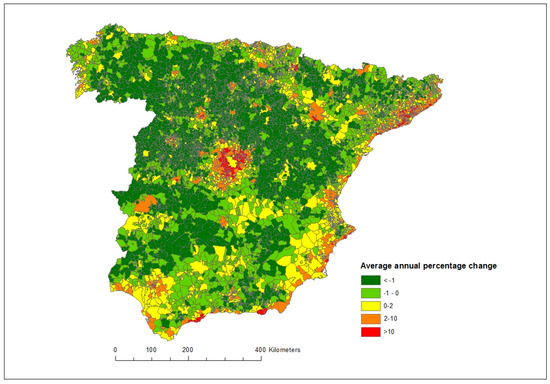
Figure 1.
Population change between 1960 and 2011.
Population concentrates increasingly in urban areas along the coast, the two main river valleys of the Guadalquivir and the Ebro and in the center around the capital Madrid, while vast parts of the country—mainly the rural interior parts—experienced population loss during this period. Although this process of population concentration had started already at the beginning of the 20th century [29], it was in the 1960s that internal migration intensified very strongly with the transition from an agricultural to an industrial economy. Migratory movements reached an unprecedented scale that profoundly changed the spatial population distribution [30,31]. Similar patterns of population concentration have also been reported for other countries, e.g., France [32].
Second, in order to distinguish between urban and rural areas, I used the recent OECD – (Organisation for Economic Cooperation and Development) [33] delimitation of functional urban areas (FUA) developed in collaboration with the EU. This classification provides a harmonized definition of FUAs for 29 OECD countries. This facilitates cross-country comparisons. Schmidheiny and Suedekum [34], for example, used this classification to compare the European to the US urban system.
The OECD classification is based on population grid data from the Corine Land Cover database and the global Landscan 2000 dataset. Based on this information, it defines FUA core areas which are contiguous or highly interconnected densely inhabited urban cores. FUA cores can have one or more urban centers of different sizes. FUA hinterlands are identified on the basis of commuting data, including all settlements from where at least 15% of the workers commute to any of the core settlements. Here, urban areas are both FUA cores plus their commuting hinterlands. The remaining municipalities that neither are core nor hinterland are classified as rural areas. The urban municipalities accounted for about 55 percent of total mainland population in 1960 and for nearly 80 percent of total mainland population in 2011. This reflects the strong urbanization process that has taken place in Spain during this period.
Third, regarding the natural geography factors that might influence local population growth differences, I used geographic information systems (GIS) to calculate a range of variables relating to four groups:
- Climate data: temperature and precipitation;
- Topographic data: ruggedness and altitude;
- Geology data: Soil and rock formations, depth to bedrock and distance to aquifers;
- Other geographic control variables: land area, longitude, latitude; distance to coast.
(a) Climate: Spain has areas with very different climatic conditions which influence land use and the potential for a given area for growth. For example, different climatic conditions will determine suitability and productivity for agricultural land use. Rainfall, for example, is critical for agricultural productivity, particularly so in the dryer climate zones. Warmer climate has been associated with greater urban growth as internal migrants are often attracted by nicer weather [5,6,9,35].
Temperature variables are based on the bioclimatic variables from the Worldclim database [36] (Version 2 with a spatial resolution of 2.5 min; aprox 4.5 km at the equator) These bioclimatic variables are derived from the original monthly temperature values averaged over the period 1970–2000. The raster data has been overlaid with the municipality layer to extract the corresponding value for each municipality centroid. I used the mean annual temperature and the temperature range for estimations.
Precipitation variables are also based on the bioclimatic variables from the Worldclim database [36] and the municipality values have been prepared in the same manner. For estimations, I used the annual precipitation and the precipitation seasonality (coefficient of variation). I have also experimented with the precipitation of the wettest month and the precipitation of the driest month. The two variables do not increase the explanatory power of the models, and main results are unchanged whether they are included or not.
(b) Topography: Topography can significantly be related to the local growth potential. Steeper and above all rugged topography makes development more costly, but also agriculture more difficult. Higher altitude and rugged topography increase the cost of infrastructure provision, and they are also often related to higher transportation costs. I included two variables to capture topographical characteristics. First, I included the altitude of the municipality measured at the municipality centroid. Second, I included a measure of terrain ruggedness based on Riley et al. [37]. For this purpose, I used the national digital terrain model (MDT200) with a 200 meters elevation grid provided by the National Geographic Institute. The Riley et al. [37] terrain ruggedness index gives a summary statistic of differences in meters in elevation and captures small-scale topographic heterogeneity.
(c) Geology: Land use patterns are furthermore influenced by soil, rock, and groundwater characteristics. Soil also influences agricultural land use. The agricultural production potential in turn can influence the urbanization process [10]. On one hand, agricultural productivity affects the opportunity costs to transfer land from agricultural land use to, for example, housing or industrial uses. On the other hand, higher agricultural productivity can free up labor to move to cities. Thus, it could be related to lower local population growth. However, higher agricultural productivity may also generate a greater local growth potential, more job opportunities, and thus attract workers and increase local population growth. I used data from the European Soil Database compiled by the European Soil Data Centre. Specifically, I used the European map of soil suitability. This data set provides a number of variables specifying the nature and properties of the soil, including a code of the most important limitations of agricultural use. From this map, I selected all cells with a Pixel value of 1 which indicates no limitation to agricultural use, and I overlaid this with the municipality layer to identify all municipalities that are in areas of no agricultural restrictions.
Soil develops from parent material. The parent material influences the structure and mineral composition of the soil in combination with climate, organism, relief, and time. Parent material exerts a big influence on soil fertility, water draining and holding capacity, erodibility, and stability of the soil. More stable soils can furthermore support greater population density [17]. Combes et al. [17] found, for example, that the dominant parent material is related to approximately one third and up to half of the variation in market potential in France. Meen et al. [20] showed for England and the two case study cities of London and Melbourne that property values reflect differences in rock formation. Here, I used again data from the European Soil Database. The data set provides a major group code for the dominant parent material of the soil typological units (STU). For Spain, there are seven different major dominant parent material classes: consolidated–clastic–sedimentary rocks, sedimentary rocks, igneous rocks, metamorphic rocks, unconsolidated deposits, eolian deposits, and organic materials. I have created polygon layers for each subgroup of dominant parent material. Next, I identified all municipality polygons that are overlaying a given dominant parent material class.
The underlying bedrock can also influence land use and development patterns. Buildings need to be anchored in the soil and bedrock, and depth to bedrock can increase construction costs [38]. Combes et al. [17] and Curci [18], for example, used bedrock depth to construct an external instrument for IV estimation in the field of agglomeration economies. The European Soil Database provides information on depth to rock, distinguishing four categories: shallow (< 40 cm), moderate (40–80 cm), deep (80–120 cm), and very deep (> 120 cm). I assigned values 1 to 4 to these four categories. I then overlaid the municipality polygon over the polygons created from the raster soil layer of depth to rock. Next, I created variables for the municipality that identify the minimum value of the depth to rock layer that is under the municipality, the maximum value, and the medium value. For example, a municipality with a maximum value of 4 has at least part of the municipality area over land with a very deep depth to rock. On the other hand, a municipality with a value of 1 has all its area of land with a very shallow depth to rock.
Aquifers have represented a crucial factor in human settlements and agriculture since the beginning of time. To identify aquifers, I first used a lithostratigraphic map provided by the Spanish Institute of Geology and Mining. From this map, I identified the characteristics of rock formations and selected carbonate, detrital, quaternary or volcanic formations of high and very high permeability. High permeability makes it easier to extract groundwater. Second, the information on underground bodies of water is based on maps from the Spanish Environment Ministry. By overlaying the lithostratigraphic map and the map of underground bodies of water, I selected all underground bodies of water that are covered by permeable rock formations. Next, I calculated the distance from each municipality centroid to the nearest underground body of water covered by these rock formations.
(d) Geography: Finally, I included geography controls for the municipality land area extension, latitude, and longitude and distance to the coast which can also be viewed as quality of life indicator.
Appendix ATable A1 provides a summary of all variables used, their definitions, and the data sources that have been used in constructing the variables.
3.2. Estimations Method
I adopted a standard population growth regression approach where I regressed municipality population change during the period of analysis on the set of natural geographical characteristics. The basic model takes the form of Equation (1):
where ∆n is the annual average log population change of municipality i during t index time periods, CLIM is the set of climate variables, TOPO is the set of topography variables, GEOLY is the set of geology variables refereeing to the soil and rock characteristics, and GEO is the set of other geographical control variables. α is the constant and β1, β2, β3, and β4 show the degree of change in the annual average log population growth for every 1-unit change in variables of CLIM, TOPO, GEOLY, and GEO, respectively.
Δni,t = α + β1CLIMi, + β2TOPOi + β3GEOLYi + β4GEOi +εi,
I calculated the average annual population growth for the period of 1960–2011 and for three subperiods of 1960–1981, 1981–2001, and 2001–2011. The natural geography characteristics are clearly exogenous to local population growth, and I therefore report below ordinary least square (OLS) estimation results.
4. Results and Discussion
Table 1 shows the results for the period of 1960–2011 for rural and urban population growth when all 20 natural geography variables are included in estimations. Table 2 provides a summary of R-squares when regressing population growth between 1960 and 2011 on the different subsets of natural geography variables. The 20 natural geography variables together capture 52 percent of the variation of population growth in rural areas and 38 percent of the variations in population growth in urban areas. The latter result is similar to that of Christensen and McCord [10], who found for China that natural geography also explains approximately 38% of the variation in urban growth between 1990 and 2000. However, part of the explanatory power of their model is driven by the initial distribution of urban land that is included in the estimations.

Table 1.
Local population growth: 1960–2011.
Table 2.
R-squares when regressing population growth between 1960 and 2011 on subsets of natural geography variables.
Climate: Both for urban and rural areas, local population growth is positively correlated with higher average temperature and a lower temperature range. This indicates that areas with more pleasant temperate climate experience more growth, and this is consistent with the findings for the US [5,9,35], Europe [6], and China [10]. However, in the regression results, once the other geography factors beyond the climate variables are included, the coefficient for mean annual temperature turns out negative in the case of rural municipalities, indicating higher population growth in areas with colder temperature. By contrast, urban population growth was related to higher mean temperature even after the inclusion of the other controls. In fact, in unconditional estimations, higher annual mean temperature is related to 29% of the variations in urban population growth. Higher annual precipitation is positively related to local population growth, while precipitation seasonality is negatively related to local population change both in urban and rural areas.
Topography: Altitude is strongly negatively related to rural population growth. Indeed, altitude alone explains 38% of the variations of population growth of rural municipalities. Ruggedness is also negatively related to rural population growth, but it adds relatively little once altitude is controlled for. In unconditional estimations for urban areas, altitude, and ruggedness are also negatively related to population growth. Here altitude relates to 23% of the local variations in population growth. However, in conditional estimations, altitude turns positive and ruggedness loses significance, indicating that other factors have been more dominant for population growth in urban areas.
Geology: Population growth in rural areas was higher in areas with no agricultural limitations, less depth to the bedrock, and in greater proximity to aquifers. Urban population growth was higher also in areas with no agricultural limitation and greater proximity to aquifers but with greater depth to the bedrock. This suggests that population growth tends to take place at the best agricultural soils [39]. Christensen and McCord [10] found for China that while urban areas are more likely to be on prime agricultural land, urban growth was less likely in areas with better agricultural land. The findings related to proximity to aquifers are also consistent with previous studies such as Burchfield et al. [9] for the US or Christensen and McCord [10] for China. As for the rock type, there are some similarities as well as differences between urban and rural population growth. In both rural and urban municipalities, population growth was stronger in areas over igneous rock and eolian deposits and lower over sedimentary rocks. As argued in Rosenthal and Strange [16], construction can be more costly on sedimentary rocks. Moreover, in rural areas, population growth was also higher in areas with unconsolidated deposits and lower in areas of organic materials.
Geography: Regarding the other geography controls, it turns out that rural population growth was higher in larger municipalities but in urban areas, population growth was actually lower in the more extensive municipalities. In both cases, population growth is negatively related to latitude. This is similar to trends in employment patterns in the US reported in Desmet and Fafchamps [40], indicating a southward move of growth. By contrast, local population growth is positively related to longitude, indicating an eastward move. Unconditionally, distance to the coast is negatively related to local population growth in both rural and urban areas. This is consistent with the population growth trends reported for Spain in Goerlich and Mas [29] for the period 1900–2001. Distance to the coast has been found to be negatively related to development in many countries (e.g. [41] for the US, [20] for England, and [10] for China) as proximity to the coast provides transportation advantages as well as environmental amenities. However, for urban population growth in Spain, once other municipality characteristics are controlled for, distance to the coast loses its significance. In this respect, the results are more in line with recent evidence for Spain reported in Gutiérrez-Posada et al. [25].
Table 3 shows the corresponding results for the three subperiods. Table 4 provides again a summary of R-squares when population growth is regressed on subsets of natural geography variables.
Table 3.
Local population growth: subperiods.
Table 4.
R-squares when regressing population growth on subsets of natural geography variables—by subperiods.
Climate: Climate explained about one third of the variation in local population growth in both rural and urban areas in the period from 1960 to 1980. Climate lost explanatory power for local population growth patterns. However, for rural areas, it continues to explain about one fifth of the variation in population growth. In fact, over time, rural population growth has become more sensitive to variations in precipitations and temperature.
Topography: Topography explained about one third of the variation in population growth both in rural and urban areas in the period from 1960 to 1980. Since then, local population growth has also become less related to topography. This was particularly evident again for urban population growth patterns.
Geology: Geology explains relatively little of local population growth patterns. For rural areas, geology relates to about 5% of the local variations in population growth. This percentage remained relatively stable. For urban population growth between 1960 and 1980, about 10% of variation has been related to geology. In all subperiods, growth was higher in areas with no agricultural restrictions and greater proximity to aquifers, lower bedrock depth in rural areas, and greater bedrock depth in urban areas. The coefficients related to rock formations maintain their sign, but significance varies in subperiods. Over time, the geology factors were also related less to urban population growth.
Geography: Geography explains nearly one fourth of the local population growth variation in rural areas. Over time, this percentage has changed little. Larger rural municipalities tend to have seen higher population growth. Latitude is again negative and longitude positive in all subperiods. Population growth in rural areas has been stronger in areas closer to the coast, also in all subperiods when only geography variables are included in the model. However, conditionally on the other sets of variables for climate, topography, and geology, distance to the coast lost its explanatory power for local population growth patterns in rural areas after 1980. In urban areas, the geography variables explained about 18% of the local population growth variations between 1960 and 1980. However, since 1980, urban population growth patterns also became less related to geography variables. Nevertheless, longitude is positive and significant in all three periods. Latitude is negative but only significant in the period of 1981–2001. Unconditionally, distance to the coast is negatively related to population growth. However, the same as with rural population growth, in urban areas too, distance to the coast lost its significance once other factors are controlled for, and in conditional estimations for the period of 2000–2011, distance to the coast actually shows a positive and significant coefficient, indicating that once other natural geography factors are controlled for in the more recent period, urban areas more distant from the coast experienced higher population growth. This pattern is most likely driven by the strong growth of the Madrid metropolitan area.
While natural geography still matters, the declining contribution of natural geography to spatial patterns of population change over time suggests that economic agglomeration factors and other second nature variables have become more significant for determining local population growth, particularly so in urban areas.
OLS could suffer from spatial autocorrelation (i.e., nearby observations are similar to each other) and spatial nonstationarity (i.e., that the average relationship obtained from a global model like the one estimate in Equation (1) might not apply to all areas). Indeed, calculating Moran’s I for residuals of the estimations of Table 1 and Table 3 shows that there is significant spatial autocorrelation. Moran’s I was calculated with Euclidean distances and different distance thresholds. With a 30 km distance threshold, Moran’s I for the urban sample and the period from 1960–2011 is, for example, 0.358, and it is significant at the 1% level using 999 permutations. For the rural sample, it is 0.184 and also significant at the 1 percent level. Moran’s I is always significant also for the different subperiods and when different distance thresholds are used. At the same time, the role of natural geography for local population growth could be context-dependent. Potential spatial heterogeneity of effects has been recognized in the local growth literature [10,25,42,43]. Geographically weighted regression (GWR) allows for both the relationship between independent and dependent variables to vary locally and to account for spatial autocorrelation [44]. GWR uses a weighting matrix for each observation based on distances around each location. Hence, GWR models the local relationships between the natural geography variables and the local population growth. It can help in improving our understanding of how natural geography characteristics relate to local population growth patterns. However, GWR is not without limitations and has been criticized for issues related to the typically unknown distance of influence, multicollinearity, and edge effects, as well as for limitations regarding causal inference. GWR estimations should thus be viewed as exploratory, as argued in Shearmur [42].
Table 5 shows the results from the geographically weighted regressions for urban population growth between 1960 and 2011. The results show that there is indeed significant geographic heterogeneity in most of the regression coefficients. Only for terrain ruggedness, agricultural soil suitability, eolian deposits and organic material formations, and land area extension, there is no significant spatial variation in the estimated coefficients.
Table 5.
Geographically weighted regression: Urban areas 1960–2011.
Appendix AFigure A1 illustrates the spatial variations in the remaining variables. Average annual temperature shows a positive coefficient everywhere, but its relationship with urban population growth is most dominant in Central Spain. A greater temperature range is negatively related to growth except in the northeast, where the coefficient turns positive. Annual precipitation shows a negative coefficient in the western part of the country and turns positive towards the northeast. Precipitation seasonality has its most dominant negative relationship with population growth in the south and east. Altitude has a negative relationship with growth in the northeast but turns positive in the rest of the country and most strongly so in the center. Regarding rock formations, consolidated rocks, sedimentary rocks, igneous rocks, and unconsolidated deposits show an east–west gradient, while metamorphic rocks show a north–south gradient. Depth to the bedrock shows its strongest relation to urban population growth in the southeast. Greater distance to aquifers has a negative relation to growth in all parts of the country but with the strongest relation in the south and southwest. The coefficients of latitude show a north–south gradient, and the coefficients for longitude a southwest–northeast gradient. Distance to coast is negative in the north but positive in the center and south.
Table 6 shows the corresponding results from the spatially weighted regressions for rural population growth between 1960 and 2011. The results show that there is also indeed significant geographic heterogeneity in most of the regression coefficients. Only for proximity to aquifers, there is no significant spatial variation in the estimated coefficients. Independent of geographical location, greater distance to aquifers shows a negative relationship with local population growth. Appendix A Figure A2 illustrates the spatial variations in the other natural geography variables for estimations of rural population growth. Most coefficients show a rather patchy geographical variation where, in many cases, the relationship of the natural geography variables with rural population growth appears mediated by proximity to main urban agglomerations.
Table 6.
Geographically weighted regression: Rural areas 1960–2011.
5. Conclusions
Spain has witnessed a rapid pace of urban development during the last few decades, accompanied by important rural depopulation. This has raised important issues for sustainability. This paper provides an analysis of long-term population change at the spatially disaggregated level and focuses on the relationship with natural geography. The results show that natural geography significantly relates to local population change, with the most relevant factors being altitude and mean annual temperature. Estimation results furthermore show that natural geography constitutes different constraints and potentials for population change in rural and urban areas. Over time, local population growth has become less related to variations in natural geography. Nevertheless, natural geography still matters, and it is still significantly related to nearly a third of the variation in local population change in rural areas. Moreover, while the overall contribution of natural geography to local population growth has declined, local population growth patterns have become more sensitive to certain climate variables. This is an important finding in the light of climate change.
Urbanization processes pose important challenges for sustainability. Such processes have important economic, social, and also environmental implications. The results in this paper indicate that population growth tends to happen on the best agricultural soils and in proximity to aquifers. Particularly in dry climate regions, such processes can also bring important challenges in terms of water vulnerability. It can put an increasing burden on the freshwater resources of the aquifers and add further to desertification processes [2]. This is particularly of concern for the Mediterranean region, where a trend towards drier conditions has been observed [45].
On the other hand, the results also indicate that the viability of rural communities is significantly related to their natural geographies. Natural geography in rural areas still contributes nearly to a third of the variation in local population change, and the negative relationship with temperature range and precipitation seasonality has even become stronger. There is evidence that global warming is changing the frequency and intensity of extreme weather events. This may further add to the declining attractiveness of rural places when people are moving away from areas with harsher weather conditions [5,46].
The results from this paper provide insights for calibrating and validating models of urban and rural growth and land use change by highlighting the role of natural geography factors. They show patterns of past local population growth, and this can be useful in understanding the occurrence of the location of future population growth. Nevertheless, the results should not be interpreted as proving causal relationships, since the natural geography factors analyzed can be correlated with socioeconomic, institutional, and political factors in determining population change patterns.
A further limitation of this study is that population growth is not disaggregated by age groups. Some geographic indicators such as distance to coast but also average temperature could be more relevant for certain age groups than for others. In future research, an age-specific approach could be adopted.
Acknowledgments
This research has greatly benefitted from support from the Fundación BBVA (Beca Leonardo a Investigadores y Creadores Culturales, 2014). Support from the Spanish Ministry of Economy, Industry and Competitiveness (ECO2016-75941R) is also acknowledged.
Conflicts of Interest
The authors declare no conflict of interest.
Appendix A
Table A1.
Definitions and data sources of the variables.
Table A1.
Definitions and data sources of the variables.
| Variables | Definition | Sources |
|---|---|---|
| Population growth 1960–2011 | log (population 2011)–log (population 1960)/51 | INE and Fundación BBVA and IVIE |
| Climate: | ||
| tempmeanAN | Annual mean temperature | WorldClim-Global Climate Data |
| temprange | Temperature annual range | WorldClim-Global Climate Data |
| precipAN | Annual precipitation | WorldClim-Global Climate Data |
| precipseason | Precipitation seasonality (coefficient of variation) | WorldClim-Global Climate Data |
| Topography: | ||
| alti | Altitude (in 100m units) | National Geographic Institute |
| rugg | Terrain ruggedness index: see Riley et al. (1999) | GIS own calculation based on National Geographic Institute data |
| Geology: | ||
| aglim | No agricultural restrictions | European Soil Database |
| rock_cons (1) | Consolidated-clastic-sedimentary rocks | European Soil Database |
| rock_sed (2) | Sedimentary rocks | European Soil Database |
| rock_ign (3) | Igneous rocks | European Soil Database |
| rock_meta (4) | Metamorphic rocks | European Soil Database |
| rock_uncons (5) | Unconsolidated deposits | European Soil Database |
| rock_eol (7) | Eolian deposits | European Soil Database |
| rock_org (8) | Organic materials | European Soil Database |
| depthmax | Depth to bedrock: max value in each municipality of 1 = shallow (< 40cm), 2 = moderate (40–80cm), 3 = deep (80– 120cm), 4= very deep (> 120cm). | European Soil Database |
| disaquif | Distance to nearest aquifer | GIS own calculation based on maps from the Spanish Institute of Geology and Mining and the Spanish Environment Ministry. |
| Geography: | ||
| area | Land area in square kilometers | INE |
| lat | Latitude | National Geographic Institute |
| long | Longitude | National Geographic Institute |
| discoast | Distance to nearest coastline | GIS own calculation |


Figure A1.
Geographically weighted regression coefficients: urban areas 1960–2011.


Figure A2.
Geographically weighted regression coefficients: rural areas 1960–2011.
References
- Domene, E.; Saurí, D. Urbanisation and Water Consumption: Influencing Factors in the Metropolitan Region of Barcelona. Urban Stud. 2006, 43, 1605–1623. [Google Scholar] [CrossRef]
- Barbero-Sierra, C.; Marques, M.J.; Ruiz-Perez, M. The case of urban sprawl in Spain as an active and irreversible driving force for desertification. J. Arid Environ. 2013, 90, 95–102. [Google Scholar] [CrossRef]
- Rodríguez-Pose, A. Dynamics of Regional Growth in Europe: Social and Political Factors; Clarendon Press: Oxford, UK, 1998. [Google Scholar]
- Krugman, P. First nature, second nature, and metropolitan location. J. Reg. Sci. 1993, 33, 129–144. [Google Scholar] [CrossRef]
- Rappaport, J. Moving to nice weather. Reg. Sci. Urban Econ. 2007, 37, 375–398. [Google Scholar] [CrossRef]
- Cheshire, P.C.; Magrini, S. Population growth in European cities: Weather matters but only nationally. Reg. Stud. 2006, 40, 23–37. [Google Scholar] [CrossRef]
- Winters, J.V.; Li, Y. Urbanisation, natural amenities and subjective well-being: Evidence from US counties. Urban Stud. 2016, 54, 1956–1973. [Google Scholar] [CrossRef]
- Wang, C. Did natural disaster affect population density growth in US counties? Ann. Reg. Sci. 2019, 62, 21–46. [Google Scholar] [CrossRef]
- Burchfield, M.; Overman, H.G.; Puga, D.; Turner, M.A. Causes of Sprawl: A Portrait from Space. Q. J. Econ. 2006, 121, 587–633. [Google Scholar] [CrossRef]
- Christensen, P.; McCord, G.C. Geographic determinants of China’s urbanization. Reg. Sci. Urban Econ. 2016, 59, 90–102. [Google Scholar] [CrossRef]
- Li, H.; Wei, Y.D.; Korinek, K. Modelling urban expansion in the transitional Greater Mekong Region. Urban Stud. 2018, 55, 1729–1748. [Google Scholar] [CrossRef]
- Ellison, G.; Glaeser, E.L. The Geographic Concentration of Industry: Does Natural Advantage Explain Agglomeration? Am. Econ. Rev. 1999, 89, 311–316. [Google Scholar] [CrossRef]
- Henderson, J.V.; Squires, T.; Storeygard, A.; Weil, D. The Global Distribution of Economic Activity: Nature, History, and the Role of Trade. Q. J. Econ. 2018, 133, 357–406. [Google Scholar] [CrossRef]
- Roos, M.W. How important is geography for agglomeration? J. Econ. Geogr. 2005, 5, 605–620. [Google Scholar] [CrossRef]
- Chasco, C.; López, A.; Guillain, R. The Influence of Geography on the Spatial Agglomeration of Production in the European Union. Spat. Econ. Anal. 2012, 7, 247–263. [Google Scholar] [CrossRef]
- Rosenthal, S.S.; Strange, W.C. The attenuation of human capital spillovers. J. Urban Econ. 2008, 64, 373–389. [Google Scholar] [CrossRef]
- Combes, P.-P.; Duranton, G.; Gobillon, L.; Roux, S. Estimating Agglomeration Economies with History, Geology, and Worker Effects. In Agglomeration Economies; Glaeser, E.L., Ed.; Chicago University Press: Chicago, IL, USA, 2010. [Google Scholar]
- Curci, F. The taller the better? Agglomeration determinants and urban structure. Mimeo 2016. Available online: https://drive.google.com/file/d/0B0Uip3oGHoIgckFqS0xGN1c5UDQ/view (accessed on 10 July 2019).
- Saiz, A. The Geographic Determinants of Housing Supply. Q. J. Econ. 2010, 125, 1253–1296. [Google Scholar] [CrossRef]
- Meen, G.; Gibb, K.; Leishman, C.; Nygaard, C. Housing Economics. A Historical Approach; Palgrave Macmillan: London, UK, 2016. [Google Scholar]
- Goerlich, F.J.; Ruiz, F.; Chorén, P.; Albert, C. Cambios En La Estructura y Localización De La Población: Una Visión De Largo Plazo (1842–2011); Fundación BBVA: Bilbao, Spain, 2015; 354p. [Google Scholar]
- Goerlich, F.J.; Mas, M. Drivers of Agglomeration: Geography vs History. Open Urban Stud. J. 2009, 2, 28–42. [Google Scholar] [CrossRef][Green Version]
- Chasco, C.; López, A. Evolution of the influence of geography on the location of production in Spain (1930–2005). In Progress in Spatial Analysis: Methods and Applications; Páez, A., le Gallo, J., Buliung, R., Dall’Erba, S., Eds.; Springer: Berlin, Germany, 2009; pp. 491–528. [Google Scholar]
- Ayuda, M.I.; Collantes, F.; Pinilla, V. From locational fundamentals to increasing returns: The spatial concentration of population in Spain, 1787–2000. J. Geogr. Syst. 2010, 12, 25–50. [Google Scholar] [CrossRef]
- Gutiérrez-Posada, D.; Rubiera-Morollon, F.; Viñuela, A. Heterogeneity in the Determinants of Population Growth at the Local Level: Analysis of the Spanish Case with a GWR Approach. Int. Reg. Sci. Rev. 2017, 40, 211–240. [Google Scholar] [CrossRef]
- Lanaspa, L.; Pueyo, F.; Sanz, F. The evolution of Spanish Urban Structure during the Twentieth Century. Urban Stud. 2003, 40, 567–580. [Google Scholar] [CrossRef]
- Le Gallo, J.; Chasco, C. Spatial analysis of urban growth in Spain, 1900–2001. Empir. Econ. 2008, 34, 59–80. [Google Scholar] [CrossRef]
- Fundación BBVA and Ivie. Series Homogéneas de Población 1900–2011. Noviembre 2015. Available online: https://www.fbbva.es/bd/cambios-la-estructura-localizacion-la-poblacion-series-homogeneas-1900-2011/ (accessed on 14 March 2019).
- Goerlich, F.J.; Mas, M. Algunas pautas de localización de la población a lo largo del siglo XX. Investig. Reg. 2008, 12, 5–33. [Google Scholar]
- Cabré, A.; Moreno, J.; Pujadas, I. Cambio migratorio y “reconversión territorial en España”. Rev. Esp. Investig. Sociol. 1985, 32, 43–65. [Google Scholar] [CrossRef]
- Bover, O.; Velilla, P. Migration in Spain: Historical Background and Current Trends; Documento de Trabajo; Banco de España: Madrid, Spain, 1999; p. 9909. [Google Scholar]
- Talandier, M.; Jousseaume, V.; Nicot, B.H. Two centuries of economic territorial dynamics: The case of France. Reg. Stud. Reg. Sci. 2016, 3, 67–87. [Google Scholar] [CrossRef]
- OECD. Redefining “Urban”: A New Way to Measure Metropolitan Areas; OECD Publishing: Paris, France, 2012. [Google Scholar] [CrossRef]
- Schmidheiny, K.; Suedekum, J. The pan-European population distribution across consistently defined functional urban areas. Econ. Lett. 2015, 133, 10–13. [Google Scholar] [CrossRef]
- Cebula, R.J.; Nair-Reichert, U.; Coombs, C.K. Total state in-migration rates and public policy in the United States: A comparative analysis of the Great Recession and the pre- and post-Great Recession years. Reg. Stud. Reg. Sci. 2014, 1, 102–115. [Google Scholar] [CrossRef]
- Fick, S.E.; Hijmans, R.J. WorldClim 2: New 1-km spatial resolution climate surfaces for global land areas. Int. J. Climatol. 2017, 37, 4302–4315. [Google Scholar] [CrossRef]
- Riley, S.J.; De Gloria, S.D.; Elliot, R. A terrain ruggedness index that quantifies topographic heterogeneity. Intermt. J. Sci. 1999, 5, 23–27. [Google Scholar]
- Barr, J.; Tassier, T.; Trendafilov, R. Depth to Bedrock and the Formation of the Manhattan Skyline, 1890–1915. J. Econ. Hist. 2011, 71, 1060–1077. [Google Scholar] [CrossRef]
- Imhoff, M.L.; Lawrence, W.T.; Elvidge, C.D.; Paul, T.; Levine, E.; Prevalsky, M.; Brown, V. Using nighttime DMSP/OLS images of city lights to estimate the impact of urban land use on soil resources in the U.S. Remote Sens. Environ. 1997, 59, 105–117. [Google Scholar] [CrossRef]
- Desmet, K.; Fafchamps, M. Changes in the spatial concentration of employment across US counties: A sectoral analysis 1972–2000. J. Econ. Geogr. 2005, 5, 261–284. [Google Scholar] [CrossRef]
- Rappaport, J.; Sachs, J.D. The United States as a Coastal Nation. J. Econ. Growth 2003, 8, 5–46. [Google Scholar] [CrossRef]
- Shearmur, R.; Apparicio, P.; Lizion, P.; Polèse, M. Space, Time, and Local Employment Growth: An Application of Spatial Regression Analysis. Growth Chang. 2007, 38, 696–722. [Google Scholar] [CrossRef]
- Partridge, M.D.; Rickman, D.S.; Ali, K.; Olfert, M.R. The Geographic Diversity of U.S. Nonmetropolitan Growth Dynamics: A Geographically Weighted Regression Approach. Land Econ. 2008, 84, 241–266. [Google Scholar] [CrossRef]
- Fotheringham, A.S.; Brunsdon, C.; Charlton, M.E. Geographically Weighted Regression: The Analysis of Spatially Varying Relationships; Wiley: Chichester, UK, 2002. [Google Scholar]
- Hoerling, M.; Eischeid, J.; Perlwitz, J.; Quan, X.; Zhang, T.; Pegion, P. On the Increased Frequency of Mediterranean Drought. J. Clim. 2012, 25, 2146–2161. [Google Scholar] [CrossRef]
- Panagopoulos, T.; Guimarães, M.H.; Barreira, A.P. Influences on citizens’ policy preferences for shrinking cities: A case study of four Portuguese cities. Reg. Stud. Reg. Sci. 2015, 2, 140–169. [Google Scholar] [CrossRef]
© 2019 by the author. Licensee MDPI, Basel, Switzerland. This article is an open access article distributed under the terms and conditions of the Creative Commons Attribution (CC BY) license (http://creativecommons.org/licenses/by/4.0/).