Contextualized Property Market Models vs. Generalized Mass Appraisals: An Innovative Approach

 ,
,  ,
,  , and
, and 
Abstract
1. Introduction
2. Background on the Main Mass Appraisal Techniques
3. Case Studies
- -
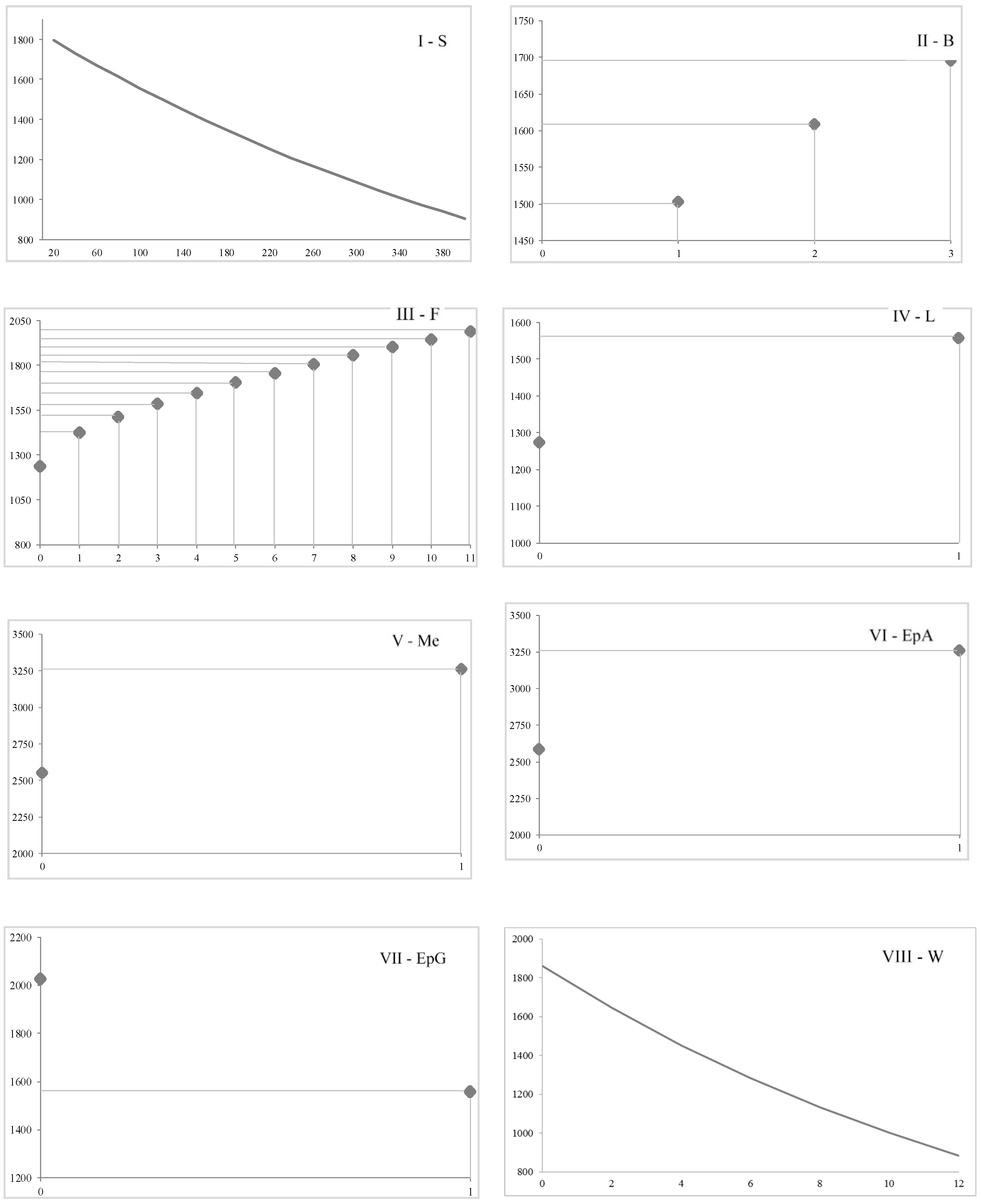
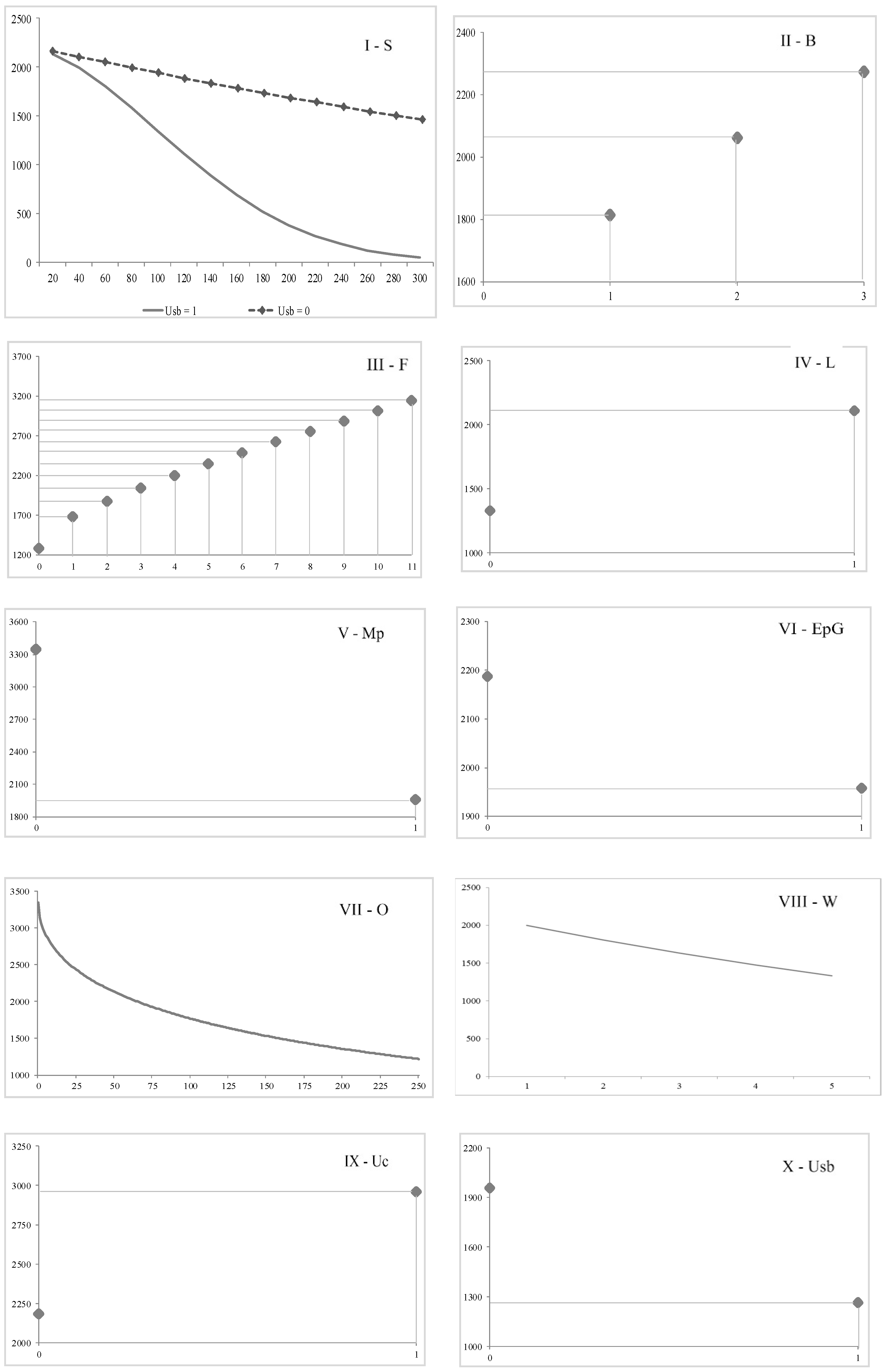
- The total surface of the property, expressed in square meters of gross floor area of the property [S];
- -
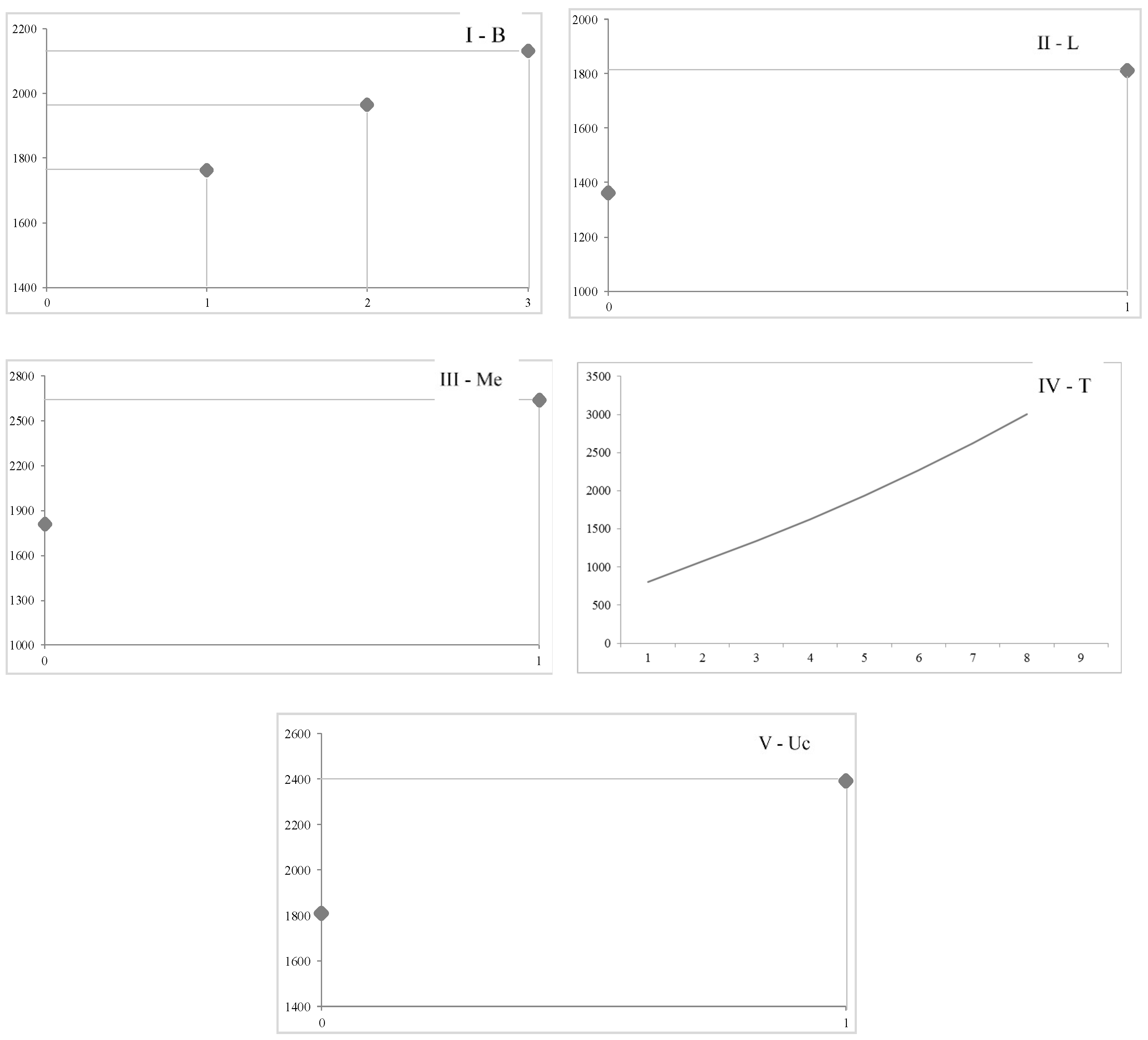
- The number of the bathrooms in the property [B];
- -
- The floor on which the property is located [F];
- -
- The presence of the lift [L]. In the model, this variable is considered as a dummy variable, in particular the presence of the service is represented by the value “one”, whereas the absence of the service is indicated with the value “zero”;
- -
- The quality of the maintenance condition of the apartment, taken as a qualitative variable and differentiated, through a synthetic evaluation, by the categories “to be restructured” [Mp], “good” [Mg], and “excellent” [Me]. Following the logic of the dummy variables, the score “one” is assigned to the category that defines the specific quality of each property, and the score “zero” for the remaining two categories [110]. In particular, the “to be restructured” state refers to properties that require significant refurbishment interventions, due to the fact that the functionality of the property is compromised by the inappropriate conditions of the elements that compose it; the “good” state indicates properties whose maintenance conditions are acceptable and whose functions can be conducted without heavy interventions. Finally, the “excellent” state refers to buildings characterized by construction and aesthetic high quality, possibly affected by recent redevelopment and renovation initiatives;
- -
- The energy performance certificate (EPC) label [Ep], expressed, according with the current regulations, through the denominations from A4 (the highest level) to G (the lowest level). In the present research, the EPC labels from A4 to A are gathered into a single explanatory variable (EpA). Therefore, the variables considered are specified by the following abbreviations, which recall the label they belong to: EpA, EpB, EpC, EpD, EpE, EpF, EpG. Each parameter is interpreted as a dummy variable, assigning a score equal to “one” to the EPC label of the property and, consequently, the score equal to “zero” to all the others;
- -
- The age of the building in which the residential unit is located [O]. This variable is calculated as the difference between the year when the property was sold (2016–2017) and the year of construction of the building.
- -
- The distance from the nearest highway, expressed in kilometers it takes to get there by car [T] (determined through the application on www.google.com/maps);
- -
- The distance from the nearest subway, expressed in kilometers it takes to walk to it [W] (determined through the application on www.google.com/maps);
- -
- The municipal trade area in which the property is located, considering the geographical distribution developed by the Italian Revenue Agency (http://www.agenziaentrate.gov.it), due to the different location characteristics that contribute to the formation of the selling prices. In particular, five trade areas are defined by the Italian Revenue Agency: “central”, “semi-central”, “peripheral”, “suburban”, and “rural”. With regard to the cities under analysis, the Italian Revenue Agency considers four trade areas: “central” [Uc], “semi-central” [Usc], “peripheral” [Up], and “suburban” [Usb]. For each property, the score “one” is assigned if the property belongs to the specific trade area, whereas the score “zero” is reported for all the remaining spatial factors.
4. The Method
5. Application of the Multi-Case Strategy for EPR Method
5.1. The Generalized Model Obtained and Its Specification to the Case Studies
5.2. Empirical Analysis of the Functional Relationships in Each City Model
6. Comparison with the Hedonic Price Method
7. Conclusions
Author Contributions
Funding
Conflicts of Interest
References
- Lohr, S. The Age of Big Data. New York Times, 11 February 2012. [Google Scholar]
- Gillespie, T. The relevance of algorithms. In Media Technologies: Essays on Communication, Materiality, and Society; Gillespie, T., Boczkowski, P.J., Foot, K.A., Eds.; MIT Press: Cambridge, MA, USA, 2014. [Google Scholar]
- Thatcher, J. Big Data, Big Questions. Int. J. Commun. 2014, 8, 1765–1783. [Google Scholar]
- Rabari, C.; Storper, M. The digital skin of cities: Urban theory and research in the age of the sensored and metered city, ubiquitous computing and big data. Camb. J. Reg. Econ. Soc. 2015, 8, 27–42. [Google Scholar] [CrossRef]
- Mostashari, A.; Arnold, F.; Mansouri, M.; Finger, M. Cognitive cities and intelligent urban governance. Netw. Ind. Q. 2011, 13, 4–7. [Google Scholar]
- Terán, L.; Kaskina, A.; Meier, A. Maturity model for cognitive cities. In Towards Cognitive Cities. Studies in Systems, Decision and Control; Portmann, E., Finger, M., Eds.; Springer: Cham, Switzerland, 2016; Volume 63, pp. 37–59. [Google Scholar]
- Dachuan, C.; Baoshan, Z. The applications of big data in housing information system. J. Inf. Commun. Technol. 2012, 5, 4. [Google Scholar]
- Juan, Y. The precise marketing based on big data in the real estate enterprises. J. Mark. Wkly. 2013, 9, 66–67. [Google Scholar]
- Du, D.; Li, A.; Zhang, L. Survey on the applications of Big Data in Chinese Real Estate Enterprise. Proced. Comput. Sci. 2014, 30, 24–33. [Google Scholar] [CrossRef]
- Stumpf González, M.A.; Torres Formoso, C. Mass appraisal with genetic fuzzy rule-based systems. Prop. Manag. 2006, 24, 20–30. [Google Scholar] [CrossRef]
- Batty, M. Smart cities, big data. Environ. Plan. B 2012, 39, 191–193. [Google Scholar] [CrossRef]
- Burgess, J.; Bruns, A. Twitter archives and the challenges of “big social data” for media and communication research. M/C J. 2012, 15, 1–7. Available online: http://www.journal.mediaculture.org.au/index.php/mcjournal/arti-cle/view/561 (accessed on 20 February 2018).
- Giddens, A. The Consequences of Modernity; Polity Press: Cambridge, MA, USA, 1990. [Google Scholar]
- Siwei, C. The fundamentals and research methods of fictitious economy. J. Manag. Rev. 2009, 21, 3–18. [Google Scholar]
- McCluskey, W.; Anand, S. The application of intelligent hybrid techniques for the mass appraisal of residential properties. J. Prop. Invest. Financ. 1999, 17, 218–238. [Google Scholar] [CrossRef]
- Pagourtzi, E.; Assimakopoulos, V.; Hatzichristos, T.; French, N. Real estate appraisal: A review of valuation methods. J. Prop. Invest. Financ. 2003, 21, 383–401. [Google Scholar] [CrossRef]
- French, N.; Gabrielli, L. Pricing to market: Property valuation revisited: The hierarchy of valuation approaches, methods and models. J. Prop. Invest. Financ. 2018, 36, 391–396. [Google Scholar] [CrossRef]
- Metzner, S.; Kindt, A. Determination of the parameters of automated valuation models for the hedonic property valuation of residential properties: A literature-based approach. Int. J. Hous. Mark. Anal. 2018, 11, 73–100. [Google Scholar] [CrossRef]
- D’Amato, M.; Kauko, T. Advances in Automated Valuation Modeling; Springer: Cham, Switzerland, 2017. [Google Scholar]
- Jud, G.D.; Winkler, D.T. Location and Amenities in Determining Apartment Rents: An Integer Programming Approach. Apprais. J. 1991, 59, 266–275. [Google Scholar]
- Des Rosiers, F.; Thériault, M. Rental Amenities and the Stability of Hedonic Prices: A Comparative analysis of Five Market Segments. J. Real Estate Res. 1996, 12, 17–36. [Google Scholar]
- Mejia, L.C.; Benjamin, J.D. What Do We Know About the Determinants of Shopping Center Sales? Spatial vs. Non-Spatial Factors. J. Real Estate Lit. 2002, 10, 3–26. [Google Scholar]
- Des Rosiers, F.; Thériault, M.; Ménétrier, L. Spatial Versus Non-Spatial Determinants of Shopping Center Rents: Modeling Location and Neighborhood-Related Factors. J. Real Estate Res. 2005, 27, 293–319. [Google Scholar]
- Emerson, F. Valuation of residential amenities: An econometric approach. Apprais. J. 1972, 40, 268–278. [Google Scholar]
- Blomquist, G.; Worley, L. Hedonic prices, demand for urban housing amenities and benefit estimates. J. Urb. Econ. 1981, 9, 212–221. [Google Scholar] [CrossRef]
- Sirmans, G.S.; Benjamin, J.D. Determining apartment rent: The value of amenities, services and external factors. J. Real Estate Res. 1989, 4, 33–43. [Google Scholar]
- Fletcher, M.; Gallimore, P.; Mangan, J. The modelling of housing submarkets. J. Prop. Invest. Financ. 2000, 18, 473–487. [Google Scholar] [CrossRef]
- Morancho, A. A hedonic valuation of urban green areas. Landsc. Urb. Plan. 2003, 66, 35–41. [Google Scholar] [CrossRef]
- Jim, C.Y.; Chen, W.Y. Impacts of urban environmental elements on residential housing prices in Guangzhou (China). Landsc. Urb. Plan. 2006, 78, 422–434. [Google Scholar] [CrossRef]
- Brander, L.M.; Koetse, M.J. The Value of urban open space: Meta-analyses of contingent valuation and hedonic pricing results. J. Environ. Manag. 2011, 92, 2763–2773. [Google Scholar] [CrossRef] [PubMed]
- Li, M.; Brown, J. Micro-neighbourhood externalities and hedonic housing prices. Land Econ. 1980, 56, 125–141. [Google Scholar] [CrossRef]
- Hickman, E.P.; Gaines, J.P.; Ingram, F.J. The influence of neighbourhood quality on residential values. Real Estate Apprais. Anal. 1984, 50, 36–42. [Google Scholar]
- Clark, D.E.; Herrin, W.E. The impact of public school attributes on home sale prices in California. Growth Chang. 2000, 31, 385–407. [Google Scholar] [CrossRef]
- Figlio, D.N.; Lucas, M.E. What’s in a grade? School report cards and the housing market. Am. Econ. Rev. 2004, 94, 591–604. [Google Scholar] [CrossRef]
- Xu, T.; Zhang, M.; Aditjandra, P.T. The impact of urban rail transit on commercial property value: New evidence from Wuhan, China. Transp. Res. Part A Policy Pract. 2016, 91, 223–235. [Google Scholar] [CrossRef]
- Yang, L.; Wang, B.; Zhang, Y.; Ye, Z.; Wang, Y.; Li, P. Willing to pay more for high-quality schools? A hedonic pricing and propensity score matching approach. Int. Rev. Spat. Plan. Sustain. Dev. 2018, 6, 45–62. [Google Scholar] [CrossRef]
- Crompton, J.L. The impact of parks on property values: A review of the empirical evidence. J. Leis. Res. 2001, 33, 1–31. [Google Scholar] [CrossRef]
- Din, A.; Hoesli, M.; Bender, A. Environmental variables and real estate prices. Urb. Stud. 2001, 38, 1989–2000. [Google Scholar] [CrossRef]
- Lutzenhiser, M.; Netusil, N.R. The effect of open spaces on a home’s sale price. Contemp. Econ. Policy 2001, 19, 291–298. [Google Scholar] [CrossRef]
- Netusil, N.R. Urban environmental amenities and property values: Does ownership matter? Land Use Policy 2013, 31, 371–377. [Google Scholar] [CrossRef]
- Kestens, Y.; Thériault, M.; Des Rosiers, F. The Impact of Surrounding Land Use and Vegetation on Single-Family House Prices. Environ. Plan. B Plan. Des. 2004, 31, 539–567. [Google Scholar] [CrossRef]
- Andersson, D.E.; Shyr, O.F.; Fu, J. Does high-speed rail accessibility influence residential property prices? Hedonic estimates from southern Taiwan. J. Transp. Geogr. 2010, 18, 166–174. [Google Scholar] [CrossRef]
- Deng, T.; Nelson, J.D. Bus rapid transit implementation in Beijing: An evaluation of performance and impacts. Res. Transp. Econ. 2013, 39, 108–113. [Google Scholar] [CrossRef]
- Shyr, O.F.; Andersson, D.E.; Li, Y.T.; Tu, C.H. The Xueshan Tunnel and the enlargement of the Taipei Metropolitan Area. Surv. Built Environ. 2018, 26, 9–31. [Google Scholar]
- Yang, L.; Zhou, J.; Shyr, O.F.; Huo, D. Does bus accessibility affect property prices? Cities 2019, 84, 56–65. [Google Scholar] [CrossRef]
- Feige, A.; Mcallister, P.; Wallbaum, H. Rental price and sustainability ratings: Which sustainability criteria are really paying back? Constr. Manag. Econ. 2013, 31, 322–334. [Google Scholar] [CrossRef]
- Taltavull de La Paz, P.; Perez-Sanchez, V.R.; Mora-Garcia, R.T.; Perez-Sanchez, J.C. Green Premium Evidence from Climatic Areas: A Case in Southern Europe, Alicante (Spain). Sustainability 2019, 11, 686. [Google Scholar] [CrossRef]
- Manganelli, B.; Morano, P.; Tajani, F.; Salvo, F. Affordability Assessment of Energy-Efficient Building Construction in Italy. Sustainability 2019, 11, 249. [Google Scholar] [CrossRef]
- Potepan, M.J. Explaining intermetropolitan variation in housing prices, rents and land prices. Real Estate Econ. 1996, 24, 219–245. [Google Scholar] [CrossRef]
- Taltavull de La Paz, P. Determinants of housing prices in Spanish cities. J. Prop. Invest. Financ. 2003, 21, 109–135. [Google Scholar] [CrossRef]
- Kryvobokov, M. What location attributes are the most important for market value? Extraction of attributes from regression models. Prop. Manag. 2007, 25, 257–286. [Google Scholar]
- Gibler, K.M.; Tyvimaa, T.; Kananen, J. The relationship between the determinants of rental housing satisfaction and considering moving in Finland. Prop. Manag. 2014, 32, 104–124. [Google Scholar] [CrossRef]
- Sdino, L.; Zorzi, F.; Rosasco, P.; Magoni, S. The Mass Appraisal Tool: Application of a Pluri-Parametric Model for the Appraisal of Real Properties. In Appraisal: From Theory to Practice; Stanghellini, S., Morano, P., Bottero, M., Oppio, A., Eds.; Springer: Cham, Switzerland, 2017. [Google Scholar]
- Boyd, D.; Crawford, K. Critical questions for big data, Information. Commun. Soc. 2012, 15, 662–679. [Google Scholar] [CrossRef]
- Kauko, T.; D’Amato, M. Mass Appraisal Methods: An International Perspective for Property Valuers; John Wiley & Sons: New Jersey, NJ, USA, 2009. [Google Scholar]
- Borst, R. Artificial neural networks: The next modelling/calibration technology for the assessment community? Prop. Tax J. 1991, 10, 69–94. [Google Scholar]
- Collins, A.; Evans, A. Artificial Neural networks: An application to residential valuation in the U.K. J. Prop. Valuat. Invest. 1994, 11, 195–204. [Google Scholar]
- Worzala, E.; Lenk, M.; Silva, A. An exploration of neural networks and its application to real estate valuation. J. Real Estate Res. 1995, 10, 185–201. [Google Scholar]
- Bonissone, P.P.; Cheetam, W.; Golibersuch, D.C.; Khedkar, P. Automated Residential Property Valuation: An Accurate and Reliable Approach Based on SoftComputing. In Soft Computing in Financial Engineering; Ribeiro, R., Zimmermann, H., Yager, R.R., Kacprzyk, J., Eds.; Physica-Verlag: Heidelberg, Germany, 1998. [Google Scholar]
- McGreal, S.; Adair, A.; McBurney, D.; Patterson, D. Neural networks: The prediction of residential values. J. Prop. Valuat. Invest. 1998, 16, 57–70. [Google Scholar] [CrossRef]
- Gallego, J. La inteligencia artificial aplicada a la valoración de inmuebles. Un ejemplo para valorar Madrid. Rev. CT/Catastro 2004, 50, 51–67. [Google Scholar]
- Kauko, T.; Hooimeijer, P.; Hakfoort, J. Capturing housing market segmentation: An alternative approach based on neural network modeling. Hous. Stud. 2002, 17, 875–894. [Google Scholar] [CrossRef]
- Do, A.Q.; Grudnitski, G. A neural network analysis of the effect of age on housing values. J. Real Estate Res. 1993, 8, 253–264. [Google Scholar]
- Islam, K.S.; Asami, Y. Housing market segmentation: A review. Rev. Urban Reg. Dev. Stud. 2009, 21, 93–109. [Google Scholar] [CrossRef]
- Byrne, P. Fuzzy analysis: A vague way of dealing with uncertainty in real estate analysis. J. Prop. Valuat. Invest. 1994, 13, 22–41. [Google Scholar] [CrossRef]
- Bagnoli, C.; Smith, H.C. The theory of fuzzy logic and its application to real estate valuation. J. Real Estate Res. 1998, 16, 169–200. [Google Scholar]
- Mao, Y.; Wu, W. Fuzzy real option evaluation of real estate project based on risk analysis. Syst. Eng. Proced. 2011, 1, 228–235. [Google Scholar] [CrossRef]
- Chang, Y.; Ko, T. An interactive dynamic multi-objective programming model to support better land use planning. Land Use Policy 2013, 36, 13–22. [Google Scholar] [CrossRef]
- Bonissone, P.P.; Cheetham, W. Financial applications of fuzzy case-based reasoning to residential property valuation. Fuzz IEEE 1997, 1, 37–44. [Google Scholar]
- Siniak, N. Fuzzy Numbers for the Real Estate Valuation. In Proceedings of the 9th European Real Estate Society Conference (ERES), Glasgow, UK, 4–7 June 2002. [Google Scholar]
- Tse, R.Y.C. An application of the ARIMA model to real estate prices in Hong Kong. J. Prop. Financ. 1997, 8, 152–163. [Google Scholar] [CrossRef]
- Makridakis, S.; Wheelwright, S.C.; Hyndman, R.J. Forecasting: Methods and Applications, 3rd ed.; John Wiley & Sons: New York, NY, USA, 1998. [Google Scholar]
- Sivitanides, P.; Southard, J.; Torto, R.G.; Wheaton, W.C. The determinants of appraisal-based capitalization rates. Real Estate Financ. 2001, 18, 27–38. [Google Scholar]
- Iacoviello, M. Consumption, house prices, and collateral constraints: A structural econometric analysis. J. Hous. Econ. 2004, 13, 304–320. [Google Scholar] [CrossRef]
- Elbourne, A. The UK housing market and the monetary policy transmission mechanism: An SVAR approach. J. Hous. Econ. 2008, 17, 65–87. [Google Scholar] [CrossRef]
- Chen, N.K.; Chen, S.S.; Chou, Y.H. House prices, collateral constraint, and the asymmetric effect on consumption. J. Hous. Econ. 2010, 19, 26–37. [Google Scholar] [CrossRef]
- Kim Hin, D.H.; Calero Cuervo, J. A cointegration approach to the price dynamics of private housing. J. Prop. Invest. Financ. 1999, 17, 35–60. [Google Scholar] [CrossRef]
- Anselin, L.; Getis, A. Spatial statistical analysis and geographic information systems. Ann. Reg. Sci. 1992, 26, 19–33. [Google Scholar] [CrossRef]
- Griffith, D.A. Advanced spatial statistics for analyzing and visualizing geo-references data. Int. J. Geogr. Inf. Syst. 1993, 7, 107–124. [Google Scholar] [CrossRef]
- Zhang, Z.; Griffith, D. Developing user-friendly spatial statistical analysis modules for GIS: An example using ArcView. Comput. Environ. Urb. Syst. 1993, 21, 5–29. [Google Scholar] [CrossRef]
- Levine, N. Spatial statistics and GIS: Software tools to quantify spatial patterns. J. Am. Plan. Assoc. 1996, 62, 381–390. [Google Scholar] [CrossRef]
- Ord, J.K.; Getis, A. Spatial autocorrelation statistics: Distribution issues and an application. Geogr. Anal. 1995, 27, 286–306. [Google Scholar] [CrossRef]
- Tiefelsdorf, M.; Boots, B. A note on the extremities of local Moran’s its and their impact on global Moran’s I. Geogr. Anal. 1997, 29, 248–257. [Google Scholar] [CrossRef]
- Dubin, R.A. Spatial autocorrelation and neighbourhood quality. Reg. Sci. Urb. Econ. 1992, 22, 433–452. [Google Scholar] [CrossRef]
- Wyatt, P.J. Using a GIS for property valuation. J. Prop. Valuat. Invest. 1995, 14, 67–79. [Google Scholar] [CrossRef]
- La Rose, T.A. Global response surface analysis used to update appraisals in a computer assisted mass appraisal environment. Presented at the World Congress III of Computer Assisted Valuation and Land Information Systems, Cambridge, MA, USA, 7–12 August 1988. [Google Scholar]
- Kettani, O.; Oral, M.; Siskos, Y. A multiple criteria analysis model for real estate valuation. J. Glob. Optim. 1998, 12, 197–214. [Google Scholar] [CrossRef]
- Kettani, O.; Khelifi, K. PariTOP: A goal programming-based software for real estate assessment. Eur. J. Oper. Res. 2001, 133, 362–376. [Google Scholar] [CrossRef]
- Estellita Lins, M.P.; De Lyra Novaes, L.F.; LoureiroLegey, L.F. Real Estate Appraisal: A double perspective data envelopment analysis approach. Ann. Oper. Res. 2005, 138, 79–96. [Google Scholar] [CrossRef]
- Adolphson, D.L.; Cornia, G.C.; Walters, L.C. Railroad property valuation using Data Envelopment Analysis. Interfaces 1989, 19, 18–26. [Google Scholar] [CrossRef]
- Król, D.; Lasota, T.; Trawiński, B.; Trawiński, K. Investigation of evolutionary optimization methods of TSK fuzzy model for real estate appraisal. Int. J. Hybrid Intell. Syst. 2008, 5, 111–128. [Google Scholar] [CrossRef]
- Wang, W.K. A knowledge-based decision support system for measuring the performance of government real estate investment. Expert Syst. Appl. 2005, 29, 901–912. [Google Scholar] [CrossRef]
- Dzeng, R.J.; Lee, H.Y. Optimizing the development schedule of resort projects by integrating simulation and genetic algorithm. Int. J. Proj. Manag. 2007, 25, 506–516. [Google Scholar] [CrossRef]
- Rezania, M.; Javadi, A.A.; Giustolisi, O. An evolutionary-based data mining technique for assessment of civil engineering systems. Eng. Comput. 2008, 25, 500–517. [Google Scholar] [CrossRef]
- Mancarella, D.; Simeone, V. Modellazione e previsione nei sistemi idrogeologici mediante la tecnica EPR (Evolutionary Polynomial Regression). G. Geol. Appl. 2008, 8, 5–16. [Google Scholar]
- Giustolisi, O.; Savic, D. Advances in data-driven analyses and modelling using EPR-MOGA. J. Hydroinf. 2009, 11, 225–236. [Google Scholar] [CrossRef]
- Morano, P.; Tajani, F.; Locurcio, M. Land use, economic welfare and property values: An analysis of the interdependencies of the real estate market with zonal and macro-economic variables in the municipalities of Apulia Region (Italy). Int. J. Agric. Environ. Inf. Syst. 2015, 6, 16–39. [Google Scholar] [CrossRef]
- Tajani, F.; Morano, P.; Ntalianis, K. Automated Valuation Models for real estate portflios: A method for the value updates of the property assets. J. Prop. Invest. Financ. 2018, 36, 324–347. [Google Scholar] [CrossRef]
- Morano, P.; Tajani, F.; Locurcio, M. GIS application and econometric analysis for the verification of the financial feasibility of roof-top wind turbines in the city of Bari (Italy). Renew. Sustain. Energy Rev. 2017, 70, 999–1010. [Google Scholar] [CrossRef]
- Tajani, F.; Morano, P.; Torre, C.M.; Di Liddo, F. An Analysis of the Influence of Property Tax on Housing Prices in the Apulia Region (Italy). Buildings 2017, 7, 67. [Google Scholar] [CrossRef]
- Tajani, F.; Morano, P.; Locurcio, M.; Torre, C.M. Data-driven techniques for mass appraisals. Applications to the residential market of the city of Bari (Italy). Int. J. Bus. Intell. Data Min. 2016, 11, 109–129. [Google Scholar] [CrossRef]
- Morano, P.; Tajani, F.; Locurcio, M. Multicriteria analysis and genetic algorithms for mass appraisals in the Italian property market. Int. J. Hous. Mark. Anal. 2018, 11, 229–262. [Google Scholar] [CrossRef]
- Grether, D.M.; Mieszkowski, P. Determinants of real estate values. J. Urb. Econ. 1974, 1, 127–145. [Google Scholar] [CrossRef]
- Gelfand, A.E.; Ghosh, S.; Knight, J.R.; Sirmans, C.F. Spatio-temporal modeling of residential sales data. J. Bus. Econ. Stat. 1998, 16, 312–321. [Google Scholar]
- McCluskey, W.J.; Deddis, W.G.; Lamont, I.G.; Borst, R.A. The application of surface generated interpolation models for the prediction of residential property values. J. Prop. Invest. Financ. 2000, 18, 162–176. [Google Scholar] [CrossRef]
- Selim, H. Determinants of house prices in Turkey: Hedonic regression versus artificial neural network. Expert Syst. Appl. 2009, 36, 2843–2852. [Google Scholar] [CrossRef]
- Janssen, C.; Yang, Z. Estimating the market value of a proposed townhouse development. J. Prop. Invest. Financ. 1999, 17, 501–516. [Google Scholar] [CrossRef]
- Bourassa, S.; Cantoni, E.; Hoesli, M. Predicting house prices with spatial dependence: A comparison of alternative methods. J. Real Estate Res. 2010, 32, 139–159. [Google Scholar]
- Bourassa, S.; Hoesli, M.; Peng, V.S. Do housing submarkets really matter? J. Hous. Econ. 2003, 12, 12–28. [Google Scholar] [CrossRef]
- Hardy, M.A. Regression with Dummy Variables. Sage Publ. 1993, 93. [Google Scholar]
- Simonotti, M. Un’applicazione dell’analisi di regressione multipla nella stima di appartamenti. Genio Rurale 1991, 2, 209–227. [Google Scholar]
- Curto, R. La quantificazione e costruzione di variabili qualitative stratificate nella multiple regression analysis (MRA) applicata ai mercati immobiliari. Aestimum 1994, 2, 195–223. [Google Scholar]
- Del Giudice, V.; De Paola, P. Spatial analysis of residential real estate rental market with Geoadditive Models. In Advances in Automated Valuation Modeling; D’Amato, M., Kauko, T., Eds.; Springer: Cham, Switzerland, 2017. [Google Scholar]
- D’Amato, M. Location value response surface model as Automated Valuation Methodology: A case in Bari. In Advances in Automated Valuation Modeling; D’Amato, M., Kauko, T., Eds.; Springer: Cham, Switzerland, 2017. [Google Scholar]
- Green, S.B. How many subjects does it take to do a regression analysis? Multivar. Behav. Res. 1991, 26, 499–510. [Google Scholar] [CrossRef] [PubMed]
- Box, G.E.; Tidwell, P.W. Transformation of the independent variables. Technometrics 1962, 4, 531–550. [Google Scholar] [CrossRef]
- Box, G.E.; Cox, D.R. An analysis of transformations. J. R. Stat. Soc. Ser. B. Methodol. 1964, 26, 211–252. [Google Scholar] [CrossRef]
- Berardi, L.; Kapelan, Z. Multi-case EPR strategy for the development of sewer failure performance indicators. In Proceedings of the World Environmental and Water Resources Congress 2007: Restoring Our Natural Habitat, Tampa, FL, USA, 15–19 May 2007; pp. 1–12. [Google Scholar]
- Cassel, E.; Mendelsohn, R. The choice of functional forms for hedonic price equations: Comment. J. Urb. Econ. 1985, 18, 135–142. [Google Scholar] [CrossRef]
- Bowes, D.R.; Ihlanfeldt, K.R. Identifying the impacts of rail transit stations on residential property values. J. Urb. Econ. 2001, 50, 1–25. [Google Scholar] [CrossRef]
- Lynch, A.K.; Rasmussen, D.W. Proximity, neighbourhood and the efficacy of exclusion. Urb. Stud. 2004, 41, 285–298. [Google Scholar] [CrossRef]
- Malpezzi, S.; Chun, G.H.; Green, R.K. New place-to-place housing price indexes for US metropolitan areas, and their determinants. Real Estate Econ. 1998, 26, 235–274. [Google Scholar] [CrossRef]
- Morano, P.; Tajani, F. Estimative analysis of a segment of the bare ownership market of residential property. In Proceedings of the 13th International Conference on Computational Science and Its Applications (ICCSA 2013), Ho Chi Minh City, Vietnam, 24–27 June 2013; pp. 433–443. [Google Scholar]
- Cropper, M.L.; Leland, B.D.; McConnell, K.E. On the choice of functional form for hedonic price functions. Rev. Econ. Stat. 1988, 70, 668–675. [Google Scholar] [CrossRef]
- Efron, B. Estimating the error rate of a prediction rule: Improvement on cross-validation. J. Am. Stat. Assoc. 1983, 78, 316–330. [Google Scholar] [CrossRef]
- Fregonara, E.; Rolando, D.; Semeraro, P. Energy performance certificates in the Turin real estate market. J. Eur. Real Estate Res. 2017, 10, 149–169. [Google Scholar] [CrossRef]
- Building Stock Observatory. 2018. Available online: https://ec.europa.eu/energy/en/eubuildings (accessed on 4 March 2018).
- D’Alpaos, C.; Bragolusi, P. Buildings energy retrofit valuation approaches: State of the art and future perspectives. Valori e Valutazioni 2018, 20, 79–94. [Google Scholar]
- Malerba, A.; Massimo, D.E.; Musolino, M.; Nicoletti, F.; De Paola, P. Post Carbon City: Building valuation and Energy Performance Simulation Programs. Smart Innov. Syst. Technol. 2019, 2019, 101. [Google Scholar]
- Oppio, A.; Bottero, M.; Arcidiacono, A. Assessing urban quality: A proposal for a MCDA evaluation framework. Ann. Oper. Res. 2018, 1–18. [Google Scholar] [CrossRef]


| Variable | Acronym | Type of Variable | Measure |
|---|---|---|---|
| Unit selling price | P | cardinal | €/m2 |
| Technical factors | |||
| Floor surface | S | cardinal | m2 |
| Number of bathrooms | B | cardinal | number |
| Floor | F | cardinal | number |
| Presence of lift | L | dummy | 1—presence, 0—absence |
| Quality of the maintenance condition of the apartment | Mp | dummy | 1—category that defines the specific quality of each property, 0—the remaining two categories |
| Mg | |||
| Me | |||
| EPC label | EpA | dummy | 1—EPC label of the property, 0—all the others |
| EpB | |||
| EpC | |||
| EpD | |||
| EpE | |||
| EpF | |||
| EpG | |||
| Age of the building | O | cardinal | Number—difference between the year of sale and the construction year of the building |
| Spatial factors | |||
| Distance from the nearest highway | T | cardinal | km by car |
| Distance from the nearest subway | W | cardinal | km by walking |
| Municipal zone | Uc | dummy | 1—if the property belongs to the specific trade area, 0—all the remaining spatial factors |
| Usc | |||
| Up | |||
| Usb | |||
| Variable | Mean | Standard Deviation | Levels/Intervals | Frequency |
|---|---|---|---|---|
| Unit selling price [€/m2] | 2244 | 812 | ||
| Technical factors | ||||
| Floor surface [m2] | 99.08 | 48.27 | ||
| <50 | 0.105 | |||
| 50–70 | 0.19 | |||
| 70–110 | 0.30 | |||
| 110–150 | 0.26 | |||
| >150 | 0.145 | |||
| Number of bathrooms [n.] | 1.485 | 0.558 | ||
| 1 | 0.545 | |||
| 2 | 0.425 | |||
| 3 | 0.03 | |||
| Floor [n.] | 2.585 | 2.264 | ||
| 0 | 0.12 | |||
| 1 | 0.335 | |||
| 2 | 0.10 | |||
| 3 | 0.165 | |||
| 4 | 0.085 | |||
| 5 | 0.065 | |||
| >5 | 0.13 | |||
| Presence of lift [1—presence, 0—absence] | 0.72 | 0.45 | ||
| 0 | 0.28 | |||
| 1 | 0.72 | |||
| Quality of the maintenance condition | To be restructured | 0.53 | ||
| Good | 0.29 | |||
| Excellent | 0.18 | |||
| EPC label | A | 0.155 | ||
| B | 0.08 | |||
| C | 0.105 | |||
| D | 0.12 | |||
| E | 0.085 | |||
| F | 0.16 | |||
| G | 0.295 | |||
| Age of the building [difference between the year of sale and the construction year of the building] | 42.51 | 2.52 | ||
| <10 | 0.285 | |||
| 10–30 | 0.11 | |||
| 30–50 | 0.19 | |||
| >50 | 0.415 | |||
| Spatial factors | ||||
| Distance from the nearest highway [km by car] | 2.775 | 1.409 | ||
| <2 | 0.315 | |||
| 2–3 | 0.265 | |||
| 3–4 | 0.18 | |||
| >4 | 0.24 | |||
| Distance from the nearest subway [km by walking] | 2.876 | 2.338 | ||
| <1 | 0.255 | |||
| 1–2 | 0.21 | |||
| 2–6 | 0.395 | |||
| >6 | 0.14 | |||
| Municipal zone | Central | 0.505 | ||
| Semi-central | 0.17 | |||
| Peripheral | 0.11 | |||
| Suburban | 0.215 | |||
| Variable | Mean | Standard Deviation | Levels/Intervals | Frequency |
|---|---|---|---|---|
| Unit selling price [€/m2] | 2992 | 1569 | ||
| Technical factors | ||||
| Floor surface [m2] | 107 | 52.02 | ||
| <50 | 0.115 | |||
| 50–70 | 0.12 | |||
| 70–110 | 0.39 | |||
| 110–150 | 0.245 | |||
| >150 | 0.13 | |||
| Number of bathrooms [n.] | 1.57 | 0.64 | ||
| 1 | 0.51 | |||
| 2 | 0.405 | |||
| 3 | 0.085 | |||
| Floor [n.] | 2.46 | 1.85 | ||
| 0 | 0.095 | |||
| 1 | 0.27 | |||
| 2 | 0.205 | |||
| 3 | 0.175 | |||
| 4 | 0.115 | |||
| 5 | 0.075 | |||
| >5 | 0.065 | |||
| Presence of lift [1—presence, 0—absence] | 0.70 | 0.46 | ||
| 0 | 0.3 | |||
| 1 | 0.7 | |||
| Quality of the maintenance condition | To be restructured | 0.305 | ||
| Good | 0.335 | |||
| Excellent | 0.36 | |||
| EPC label | A | 0.185 | ||
| B | 0.045 | |||
| C | 0.085 | |||
| D | 0.055 | |||
| E | 0.11 | |||
| F | 0.255 | |||
| G | 0.265 | |||
| Age of the building [difference between the year of sale and the construction year of the building] | 70.50 | 57.25 | ||
| <10 | 0.14 | |||
| 10–50 | 0.24 | |||
| 50–80 | 0.335 | |||
| >80 | 0.285 | |||
| Spatial factors | ||||
| Distance from the nearest highway [km by car] | 3.29 | 1.52 | ||
| <2 | 0.19 | |||
| 2–3 | 0.35 | |||
| 3–4 | 0.225 | |||
| >4 | 0.235 | |||
| Distance from the nearest subway [km by walking] | 1.20 | 1.04 | ||
| <0.5 | 0.295 | |||
| 0.5–1 | 0.315 | |||
| 1–3 | 0.335 | |||
| >3 | 0.055 | |||
| Municipal zone | Central | 0.34 | ||
| Semi-central | 0.35 | |||
| Peripheral | 0.135 | |||
| Suburban | 0.175 | |||
| Variable | Mean | Standard Deviation | Levels/Intervals | Frequency |
|---|---|---|---|---|
| Unit selling price [€/m2] | 2468 | 1316 | ||
| Technical factors | ||||
| Floor surface [m2] | 79.39 | 44.33 | ||
| <50 | 0.27 | |||
| 50–70 | 0.295 | |||
| 70–110 | 0.27 | |||
| 110–150 | 0.105 | |||
| >150 | 0.06 | |||
| Number of bathrooms [n.] | 1.21 | 0.45 | ||
| 1 | 0.81 | |||
| 2 | 0.17 | |||
| 3 | 0.02 | |||
| Floor [n.] | 2.41 | 1.64 | ||
| 0 | 0.045 | |||
| 1 | 0.335 | |||
| 2 | 0.19 | |||
| 3 | 0.215 | |||
| 4 | 0.095 | |||
| 5 | 0.09 | |||
| >5 | 0.03 | |||
| Presence of lift [1—presence, 0—absence] | 0.75 | 0.44 | ||
| 0 | 0.255 | |||
| 1 | 0.745 | |||
| Quality of the maintenance condition | To be restructured | 0.23 | ||
| Good | 0.29 | |||
| Excellent | 0.48 | |||
| EPC label | A | 0.235 | ||
| B | 0.055 | |||
| C | 0.17 | |||
| D | 0.22 | |||
| E | 0.11 | |||
| F | 0.075 | |||
| G | 0.135 | |||
| Age of the building [difference between the year of sale and the construction year of the building] | 83.25 | 74.03 | ||
| <10 | 0.14 | |||
| 10–50 | 0.24 | |||
| 50–80 | 0.33 | |||
| >80 | 0.29 | |||
| Spatial factors | ||||
| Distance from the nearest highway [km by car] | 4.99 | 1.38 | ||
| <3 | 0.13 | |||
| 3–5 | 0.345 | |||
| 5–6 | 0.275 | |||
| >6 | 0.25 | |||
| Distance from the nearest subway [km by walking] | 1.57 | 1.15 | ||
| <0.5 | 0.235 | |||
| 0.5–1 | 0.185 | |||
| 1–3 | 0.465 | |||
| >3 | 0.115 | |||
| Municipal zone | Central | 0.30 | ||
| Semi-central | 0.48 | |||
| Peripheral | 0.22 | |||
| Suburban | 0.00 | |||
| Polynomial Expression Structure | |
| Inner Function f | No function f |
| Modeling Type | Statical Regression |
| Maximum Number of Terms | 10 |
| Exponents | [−2, −1.5, −1, −0.5, 0, 0.5, 1, 1.5, 2] |
| Regression Method | LS (Least Squares) |
| Equation (n) | Model | CODMCS [%] |
|---|---|---|
| (3) | 60.00 | |
| (4) | 63.78 | |
| (5) | 65.89 | |
| (6) | 66.13 | |
| (7) | 69.60 | |
| (8) | 70.87 | |
| (9) | 71.28 | |
| (10) | 72.34 | |
| (11) | 78.32 |
| a0 | a1 | a2 | a3 | a4 | a5 | a6 | a7 | a8 | a9 | a10 | |
|---|---|---|---|---|---|---|---|---|---|---|---|
| BARI | 7.59 | 0 | 0 | −0.49 | 0.23 | 0.24 | 0 | 0.14 | 0.16 | −0.0006 | 0 |
| ROME | 7.42 | 0.30 | 0 | 0 | 0 | 0 | −0.06 | 0.27 | 0.37 | −0.0009 | −3.8E-05 |
| TURIN | 5.50 | 0.28 | 0.77 | 0 | 0 | 0.38 | 0 | 0 | 0.26 | 0 | 0 |
| Model | RMSE [%] | MAPE [%] | MaxAPE [%] | |
|---|---|---|---|---|
| BARI | 4.03 | 2.41 | 9.62 | |
| ROME | 3.89 | 3.02 | 8.37 | |
| TURIN | 4.15 | 2.58 | 8.24 |
| BARI | ROME | TURIN | ||||
|---|---|---|---|---|---|---|
| Training Set | Validation Set | Training Set | Validation Set | Training Set | Validation Set | |
| Iteration 1 | 2.545 | 2.985 | 2.985 | 3.254 | 3.021 | 3.245 |
| Iteration 2 | 2.816 | 2.657 | 2.835 | 3.327 | 2.854 | 2.745 |
| Iteration 3 | 3.120 | 3.247 | 3.021 | 2.989 | 2.968 | 3.040 |
| Iteration 4 | 3.058 | 3.049 | 3.254 | 3.654 | 2.476 | 2.847 |
| Iteration 5 | 2.459 | 2.843 | 3.115 | 3.018 | 3.124 | 2.980 |
| Iteration 6 | 2.847 | 2.642 | 3.541 | 3.899 | 3.016 | 3.124 |
| Iteration 7 | 2.012 | 2.451 | 3.095 | 3.367 | 2.012 | 2.743 |
| Iteration 8 | 2.267 | 2.897 | 2.999 | 3.253 | 2.915 | 2.802 |
| Iteration 9 | 3.196 | 3.074 | 3.001 | 2.899 | 3.047 | 3.000 |
| Iteration 10 | 3.087 | 3.547 | 3.152 | 3.473 | 2.682 | 3.086 |
| S | B | F | L | Mp | Me | EpA | EpG | O | T | W | Uc | Usb | |
|---|---|---|---|---|---|---|---|---|---|---|---|---|---|
| BARI |  | | | | | | | | |||||
| ROME | | | | | | | | | | | |||
| TURIN | | | | | |
| Variable | Coefficient | Significance |
|---|---|---|
| constant | 7.5181 | *** |
| S | −0.0006 | - |
| B | 0.0108 | - |
| F | 0.0136 | - |
| L | 0.2304 | *** |
| Me | 0.2479 | *** |
| EpA | 0.2127 | *** |
| EpG | −0.2736 | *** |
| W | −0.0403 | *** |
| Variable | Coefficient | Significance |
|---|---|---|
| constant | 7.2210 | *** |
| S | 0.0008 | - |
| B | 0.0810 | - |
| F | 0.0338 | ** |
| L | 0.4320 | *** |
| Mp | −0.0652 | - |
| EpG | −0.0607 | - |
| W | 0.1160 | *** |
| O | −0.0009 | * |
| Uc | 0.2697 | *** |
| Usb | −0.5254 | *** |
| Variable | Coefficient | Significance |
|---|---|---|
| constant | 6.1522 | *** |
| B | 0.1196 | *** |
| L | 0.2630 | *** |
| Me | 0.3748 | *** |
| T | 0.1840 | *** |
| Uc | 0.2684 | *** |
© 2019 by the authors. Licensee MDPI, Basel, Switzerland. This article is an open access article distributed under the terms and conditions of the Creative Commons Attribution (CC BY) license (http://creativecommons.org/licenses/by/4.0/).
Share and Cite
Morano, P.; Rosato, P.; Tajani, F.; Manganelli, B.; Di Liddo, F. Contextualized Property Market Models vs. Generalized Mass Appraisals: An Innovative Approach. Sustainability 2019, 11, 4896. https://doi.org/10.3390/su11184896
Morano P, Rosato P, Tajani F, Manganelli B, Di Liddo F. Contextualized Property Market Models vs. Generalized Mass Appraisals: An Innovative Approach. Sustainability. 2019; 11(18):4896. https://doi.org/10.3390/su11184896
Chicago/Turabian StyleMorano, Pierluigi, Paolo Rosato, Francesco Tajani, Benedetto Manganelli, and Felicia Di Liddo. 2019. "Contextualized Property Market Models vs. Generalized Mass Appraisals: An Innovative Approach" Sustainability 11, no. 18: 4896. https://doi.org/10.3390/su11184896
APA StyleMorano, P., Rosato, P., Tajani, F., Manganelli, B., & Di Liddo, F. (2019). Contextualized Property Market Models vs. Generalized Mass Appraisals: An Innovative Approach. Sustainability, 11(18), 4896. https://doi.org/10.3390/su11184896