1. Introduction
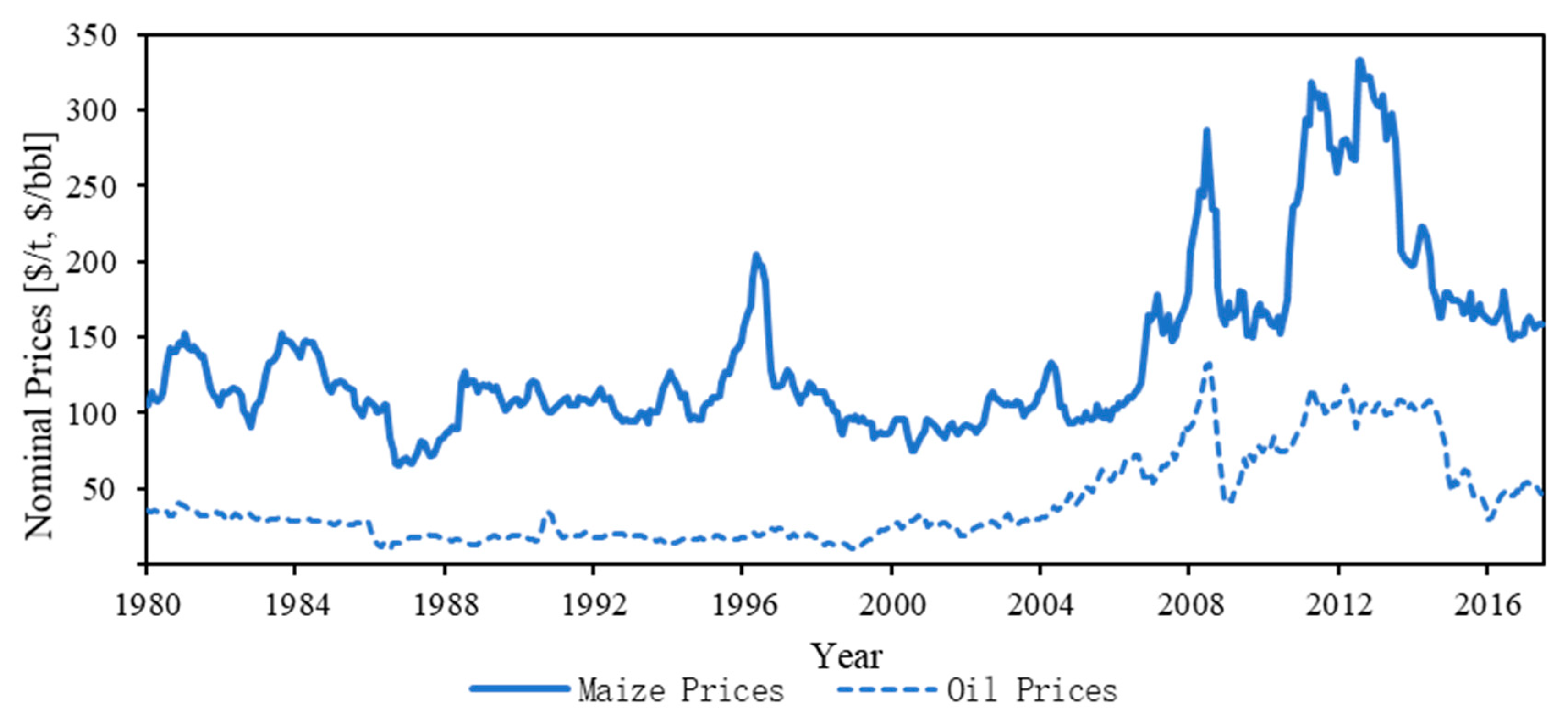
With the development and application of science and technology in energy and agriculture, the link between oil price and food price becomes complex and strong. Among all the crops in this relationship, maize could be the most representative, and it plays an important role. On the one hand, fossil energy, represented by oil, is involved in the production and circulation of food such as maize directly or indirectly, and oil price make up the cost of production and circulation of maize. In modern agricultural production, farmers replace other factors by increasing the investment capital in various forms, including agricultural machinery, energy power, fertilizers, pesticides, etc., which are direct products of the petrochemical industry, or closely related. On the other hand, fossil energy causes the derived demand for maize, which affects the price of maize and other foods. The development of the bioenergy industry (such as the ethanol fuel industry) has brought biocrops such as maize into energy production activities directly, where maize becomes an input to bioenergy, which is a substitute for petroleum products. The biocrops have changed the food market as never before. In addition, both oil and maize are commodities, and their prices are affected by macroeconomic factors, especially when the financial attributes of the commodities increase gradually.
Figure 1 shows an increasingly relevant trend between oil prices and maize prices in such a complicated relationship.
The similar price volatility in oil and food markets raises the worry and questions about their links: how do oil prices affect food prices, such as maize? And, how does the development of bioenergy change this effect?
Discussions on this issue have been around for a long time. As early as the end of the 1980s, the relationship between the oil market and the food market has been discussed. However, because of the budding development of bioenergy, the relationship between oil and food was relatively simple, and the research also just revealed a simple causal relationship [
1]. Although oil prices have been confirmed through extensive research to affect food prices, such as maize prices, through cost channels [
2,
3], the increasingly violent fluctuations in food prices, especially since the international food crisis in 2006 and the accompanying rise in food prices, has brought attention from many scholars to this issue. Scholars began to doubt the simple influence described above and proposed various theories. One focus is how oil prices affect the prices of maize and other foods, i.e., whether the development of bioenergy leads to an increase in the prices of maize and other foods. Some scholars believe that the development of bioenergy makes the conflict with the food supply worse. For example, Brown [
4] claimed that the development of the ethanol fuel industry will stimulate the world food prices like never before. Mitchell [
5] estimated that the rapid growth of bioenergy in Europe and the United States contributed 70% of the increase in world food prices, which is similar to the conclusions of Lipsky [
6]. This positive effect on food prices was confirmed by other analyses [
7,
8,
9,
10]. However, some studies have shown that the impact of oil prices on food prices via the demand for bioenergy is not as intense as indicated above but is short-term, mild, or does not affect food prices, and the production cost channel is mainly affected rather than the derived demand channel, especially as the new bioenergy technology reduces this derived demand for food [
11,
12,
13,
14,
15,
16].
In short, a key point in the studies is whether the development of bioenergy will aggravate the rising prices of food such as maize when the oil price is growing.
Although the literature fails to agree on the answer to this question, two obvious and direct channels through which oil prices influence maize prices are summarized: (production) the cost channel and (derived) the demand channel. However, some points remain debatable in the theoretical and empirical analysis. As for the theoretical analysis, most studies ignore the threshold conditions of the demand channel. That is, the demand channel will work only when the production of bioenergy is relatively more profitable than fossil energy, or if the effect of the demand channel does not exist, as with empirical analysis, the interaction between the oil prices and maize prices (or food prices) is ignored, which may lead to an endogenous problem.
Therefore, this study first constructs a petroleum price–maize price model that combines the cost channel and the demand channel and then it establishes the threshold conditions for the demand channel to play a role in the model, thereby theoretically analyzing the impact of oil prices on maize prices. Then, the empirical analysis is carried out in combination with the price data, and the estimation bias problem that may exist in the model is overcome, and the robustness test is designed to further ensure the model estimation result. These efforts are a positive complement to existing research, re-examining the complex relationship between oil prices and food prices, such as for maize, and answering the question of whether the development of biomass energy would exacerbate the problem of rising maize prices because of rising oil prices.
This article considers the relationship between oil prices and maize prices in many ways, although some points are adopted from other studies. The threshold condition for demand channel of the effects on maize prices by oil prices has rarely been incorporated, except by Ciaian and Kancs [
9]. In this paper, a model is used that could infer the important and interesting result that developing bioenergy would not exacerbate the price increase of maize, and a negative feedback mechanism of developing bioenergy is proposed. Most empirical research results about this issue did not overcome the endogenous problem, and thus the causality of the results may be biased. This paper tries to avoid this problem by keeping the model above unchanged. This paper also provides evidence about the empirical threshold.
The rest of the paper is organized as follows:
Section 2 introduces the theoretical model construction and analyzes the impact of oil prices on maize prices based on this model.
Section 3 discusses the influence by empirical analysis, including benchmark regression, and some robustness analyses. All these empirical analyses are based on the theoretical model in
Section 3. The last section concludes this paper.
2. Theoretical Framework
How do oil prices affect food prices in theory? For researchers, an equilibrium model is adopted generally for the analysis of the effect of oil prices on maize prices [
10,
17,
18,
19,
20]. Earlier, Gardner et al. [
21] considered the cross-price elasticity among biomass, ethanol, and fossil energy. Gorter and Just [
22,
23,
24] linked oil prices to bioenergy prices by considering the profit maximization of bioenergy suppliers. However, the studies above only focused on the cost of agricultural production, which we earlier defined as the cost channel. An important contribution to the theoretical model comes from Chen et al. [
25], a study that added the demand channel, building a model consisting of both the cost and demand channels. Ciaian and Kancs [
9] made an important further expansion to Gardner et al. 21 and Gorter and Just [
22,
24] by adding consideration of a price competition between biofuel and fuel into the model. The theoretical analysis of this paper is constructed with reference to the model of Ciaian and Kancs [
9].
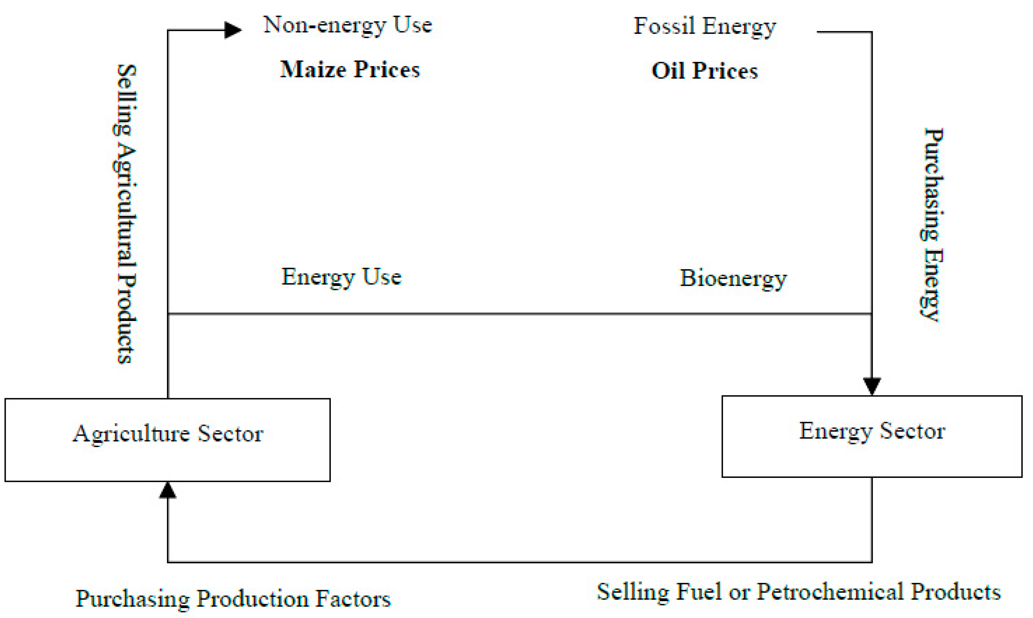
The relationship between oil prices and maize prices, considering the cost and the demand channels, is shown in
Figure 2. At first, an economy with two sectors—energy and agriculture sectors—is assumed. In the agricultural product market, the maize produced by the agricultural sector is mainly sold to two consumers: one consumer uses maize for traditional non-energy uses such as food and feed, and the other uses maize for bioenergy. In the agricultural factors market, agricultural producers purchase fuel, chemical fertilizers, pesticides, machinery, and other petrochemical products or related products; in the energy factors market, energy producers purchase fossil energy or biomass; and in the energy product market, energy producers sell their fuel or related petrochemical products, such as chemical fertilizer, pesticides, and machinery, to agricultural producers directly or indirectly. Through the cost channel and the demand channel, i.e., the products market and factors market, the agriculture sector and energy sector are connected, and the oil prices will influence the maize prices. In addition, the markets are clear.
For the agriculture sector, this study is based on the cropland allocation model of McConnell [
26], Gardner et al. [
21], and Chen et al. [
25], and the model assumes that the agricultural producers need to allocate their limited land (the limited land assumption is actually a strong assumption, because farmers would reclaim land or adjust their planting crops if producing maize is more profitable. There is some evidence to support the increase in maize planting. However, weakening this assumption has little effect on our conclusions, because planting more maize would slow down the maize price increase, that is, a weaker assumption here means a smaller effect of developing bioenergy on the maize price increase than our theoretical results. This makes our results more credible) to produce maize for non-energy use (NM) and energy use (EM). We further assume that no differences exist between these two kinds of maize when they are produced; that is, they have the same production condition and yields. The prices are respectively
and
, the outputs are
and
, and the total output of maize is
. The demand for maize, in the non-energy use market, i.e., the traditional agricultural product market, is
, and its inverse demand function is as follows:
It is assumed that agricultural production requires two inputs, one is fuel (and petrochemical products), indicated by
fuelA, and the other one, which is not related to the energy sector, is represented by land, indicated by
L. The quantities of these two inputs are
with
. As we assumed above, the inputs and technology of producing
NM and
EM are similar. We assume that the production function is
, and the total supply quantity of maize in the agriculture sector is
, which is determined as follows:
This means that maize output is dependent on the amount of fuel and land inputs. Furthermore, if land is constant, the maize output depends only on the amount of fuel. We set the demand for fuel in the agriculture sector to
and the fuel price to
, so the inverse demand function is as follows:
We set the unit land rent to
, and then the profit function of the agriculture sector is as follows:
The first-order optimal condition of the profit function is as follows:
The yield of maize varies with the amount of fuel input, i.e.,
, therefore:
The equilibrium for facing two maize markets requires the following:
For the energy sector, when we assume that only one product “fuel” is produced, whose output is
and price is
, whereas the demand for fuel is
, the inverse demand function is as follows:
The production of fuel requires raw materials
, whose quantity is
. We assume that two sources of homogeneous materials exist, which could fully substitute for each other, with bioenergy raw materials being indicated by
BO and fossil energy raw materials being indicated by
FO. The quantity is, respectively,
and
. The total demand for raw materials
is
:
where the demand for
FO (such as oil) is related to its price as determined below:
Similarly, the production of the energy sector follows a production function
:
Therefore, the profit function of the energy sector is as follows:
The first-order optimal condition is as follows:
Similarly, the production of fuel is related to the inputs of raw materials, namely:
, therefore the following:
Because the bioenergy raw materials
BO and fossil energy raw materials
FO can substitute for each other fully, the equilibrium requires the following:
Considering the formulas (8), (13), and (14), a relationship between fuel prices and fossil energy prices is as follow:
The demand for bioenergy raw materials of the energy sector, indicated by
, comes from the insufficient supply of fossil fuels; therefore, this demand equals the difference between the demand for total energy
and fossil energy
FO:
is set as the conversion rate of maize to its bioenergy equivalent to fossil energy, so the supply of bioenergy raw materials is as follows:
In general, considering the conversion rate, if the price of bioenergy raw materials is higher than the price of fossil energy raw materials, a rational energy producer will not use biomass energy raw materials, and bioenergy will not be in demand. Referring to Ciaian and Kancs [
9], this paper believes that the demand for bioenergy will occur only when its price is not higher than the fossil energy price. Thus, we set an indicator function
: if
, then
; otherwise
. Therefore, the actual demand for bioenergy of the energy sector is as follows:
The demand for maize for energy use is
:
Considering the formulas (1), (15), (2), (16), and (19), the following results are derived:
Obviously, in the formula (20), the non-energy use maize price depends on the fossil energy price . However, the relationship between the non-energy use maize price and the fossil energy price is also related to the production function of agriculture and energy sector, as indicated by and .
Let us assume a function in the form of Cobb–Douglas for
, and a function in which the output is directly proportional to the quantity of raw materials for
:
Because the land is constant, the formula (20) could be simplified as follow:
where
,
,
,
,
.
As a power function item is included in formula (23), an approximation is obtained by taking the nth-order terms of a Taylor series expansion at
for the power function term:
Then, the following formula is a simplified function of non-energy use maize price
relative to the fossil energy price
:
where
, which is equivalent to
, where
a threshold variable, and
is the threshold value.
The theoretical model tells us some facts we already knew. The first one is that the fossil energy (oil) prices do impact maize prices. The second one is that the effect of oil prices on maize prices works through two channels: cost and demand. Oil prices could affect the factor allocation and total cost of agricultural production, and then affect the maize prices, which is called the cost channel. Oil prices also affect the demand for bioenergy and cause the demand for maize for energy use, which is called the demand channel. Both channels may work.
In addition, this theoretical approach also shows us some other truths. A very important one is that a threshold or a trigger exists in this influence. The threshold compares the bioenergy prices to fossil prices and determines whether the demand channel would work. This means that, even if the oil prices are rising, the demand channel may not work at all. As shown in formula (25), equals zero, and two terms fail to contribute to the dependent variable. Because of this threshold, the demand channel does not seem to affect maize prices intensely. It means that developing bioenergy does not have a long-term serious pulling effect on maize prices; if the oil prices are relatively high and maize prices are low, possibly with oil prices rising sharply, an energy producer would face a rising cost of using fossil oil, and producing bioenergy would be more profitable, so the threshold would open the demand channel, which would raise the lower maize prices and restrict the oil price increase. However, if the oil prices are relatively low and maize prices are high, possibly with maize prices rising sharply, an energy producer could use fossil oil at a relatively low price, and the threshold would close the demand channel and slow down the increase in maize price, which would reduce the demand for energy-use maize and restrict the maize price increase. That is, through the demand channel, the relationship between oil prices and maize prices becomes closer, and this channel is more like a stabilizer than an intensifier, because of its negative feedback mechanism.
These results will be empirically validated in the next section.
3. Empirical Analysis
3.1. Data, Variables, and Model
The main data are the monthly global price data for oil and maize from the International Monetary Fund (IMF). The oil price is calculated on average from the Brent crude oil price, the West Texas Intermediate crude oil price and the Dubai crude oil price. From January 1980 to June 2017 (this is a long period for this research. Some changes in this long period may influence the analysis. To alleviate this worry, two parts of robustness test use a shorter period, which is the focus period of most studies (see regression 8 to 11 in Table 4), 450 observations were obtained. As these time series are too long, these prices are influenced by a complex set of factors of the macroeconomic environment, and the price data need to be deflated to eliminate or weaken the impact of currency prices and some macroeconomic changes on commodity price changes. The month-on-month core consumer price index (core CPI) released by the United States Department of Labor is used.
Some serious problems need to be solved. Time series data may have serial correlation problems and heteroscedasticity problems, and as shown in the previous analysis, endogeneity is obviously due to an interaction between maize prices and oil prices. A feasible generalized least squares estimation (feasible GLS, FGLS) provides a solution to heteroscedasticity or serial correlation problems, and its estimators are uniform and asymptotic. Rao and Griliches [
27] proved that the estimators of FGLS are better than Ordinary Least Squares (OLS) when the serial correlation problem is serious. Stock and Watson [
28] proposed dynamic OLS (DOLS), a new estimation method by adding the lag term and lead term of the first-order difference term of the independent variable, which eliminates the interference of the lag or lead term on the residuals. DOLS overcomes the problems with endogeneity and serial correlation. Furthermore, the use of the feasible generalized least squares method to estimate this model with lead and lag terms is called the dynamic feasible generalized least squares method (dynamic feasible GLS, DFGLS). Using this method, the estimators are unbiased, efficient, and uniform, even if the prior model is endogenous [
29].
Formula (25), in the theoretical analysis, has more than n items. The choice of n is a trade-off between fitting precision and the degree of freedom. To determine the form of the Taylor series expansion, this paper attempts to expand from 1st to 4th order, then choose the best one according to the Akaike information criterion (AIC) and Bayesian information criterion (BIC), shown in
Table 1. The optimal expansion order of the model is 1st order.
The 1st order terms of a Taylor series expansion model is:
where
and
are the maize prices and oil prices at the
t-th, period respectively,
is the indicator described above, and
is the residual. When the indicator
, oil prices only affect maize prices through cost channel,
indicates the marginal effect of oil prices through the cost channel. Otherwise, when the indicator
, the demand channel will work,
and
indicate the effect of oil prices through the demand channel. If
and
are positive and statistically significant, this proves that developing bioenergy does exacerbate the price increase of maize caused by rising oil prices. Otherwise, this assertion is not supported, and if the Taylor expansion is more than 1st order, consideration of the coefficients of all the terms with the indicator
is necessary.
The formation and fluctuation of maize and other food prices is complicated. This study attempts to control these complex influencing factors or weaken their influence on the empirical results. First, some shocks, such as severe meteorological disasters, crop diseases, and insect pests, shock the food prices, especially annual prices. Utilizing the characteristics of production cycle and analyzing a long-term month-on-month change data could weaken these uncertain shocks on price change. Second, we eliminate some macro factors reflected in the price index by deflating. Third, we use wheat prices to control other confounding factors. Wheat and maize are both bulk crops, they can both be consumed as food or feed, and the conditions of their production, such as the natural environment and mechanical work, are similar. Thus, controlling wheat prices could exclude many potential factors that are hard to measure. Luckily, a fundamental difference exists in the energy market between maize and wheat, whereby wheat is rarely use as bioenergy. Therefore, controlling wheat prices would not indicate interference in the empirical analysis.
Before the regression estimation, some work must be done on the variables.
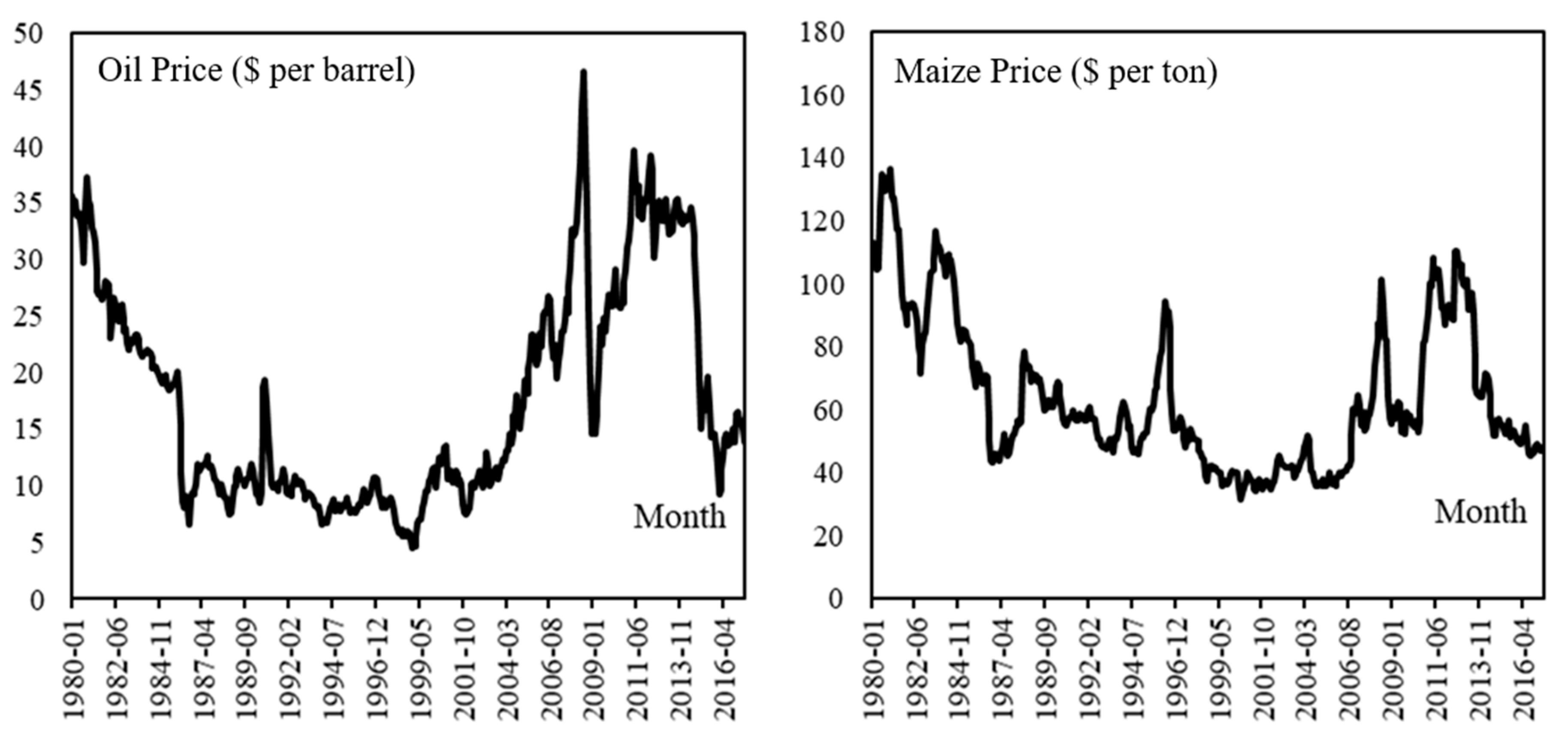
The first is that we must test the stationary or cointegration of the time series variables. As shown in
Figure 3, the price variables,
and
are both almost stable with a trend, so a trend term and an intercept term are added to the unit root test. The augmented Dickey–Fuller (ADF) unit root test results show that both
and
are stationary. In the unit root test, the lag orders, determined according to AIC and BIC, are both one period. The results show that the value of t-test of
and
are −2.862 and −2.804, significant at the 1% level. An ADF test without intercept term was also taken, the results show that the variables are still significant.
Secondly, we need to confirm the causal relationship of the variables. The correlation coefficient between the maize price and oil price is 0.6411, showing a positive correlation. The Granger causality tests show that the oil price will cause the maize price, but this is not a reverse causal relationship.
3.2. Benchmark Model Results
Table 2 shows the benchmark model estimation results of the impact of oil prices on maize prices. Ignoring the threshold, maize price has a long-term positive relation with oil price, shown in regression (1).
According to Hansen [
30,
31,
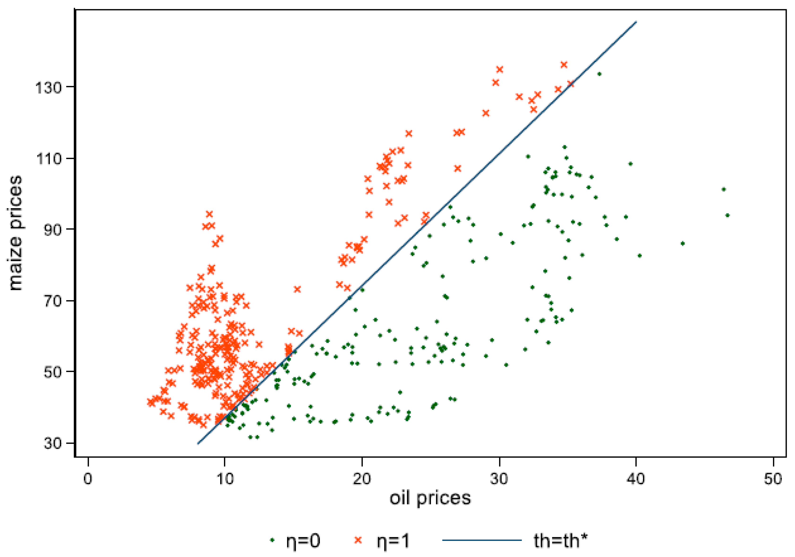
32], the threshold,
, is 3.7098. All data points could be divided into two different fields by the threshold, as shown in
Table 3 and
Figure 4. When the threshold variable is less than 3.7098, the relative price of maize price to oil price is lower, and producing bioenergy is profitable. Both cost channel and demand channel will work. When the threshold variable is greater than 3.7098, the relative price of maize price to oil price is higher, and only the cost channel will work.
Considering the threshold effect, regressions (2) to (5) are the results of the estimating formula (26) when using the different methods. For example, different results are obtained when using FGLS and DFGLS, which means that, if the problem of endogeneity is not considered, the results will be biased. The results show that the coefficient of impact of oil price is positive and significant at the 1% level, whereas the cross term of the indicator and oil price and the cross terms of the indicator and the constant term are not statistically significant. The results imply that oil prices have a significant positive impact on maize prices through the cost channel and the demand channel. However, in the long term, the positive effects mainly work through cost demand. Although the development of bioenergy indeed changes the demand for maize, it has only limited impact on maize prices. This is consistent with the result of the theoretical analysis.
Some earlier empirical data indicated that the economical threshold of using maize to produce bioenergy diverged from $36 per barrel to $45 per barrel. Notably, our threshold means an economic development of bioenergy only when the maize prices (USD/ton) is less than 3.7098 times the oil prices (USD/barrel). Compared to the empirical threshold data, this threshold takes the price changes of oil and maize into account. If we transfer our threshold value, 3.7098, to an average nominal price with the same period of those empirical data, the threshold will be $34.4357 per barrel, which is close to the empirical threshold data.
3.3. Robustness Test
Some problems, mentioned earlier, will influence the empirical model and results, which requires discussion to ensure the accuracy. The priority aim of robustness is to test whether the demand channel will work in the long term.
The first robustness test is to adjust the order of the Taylor series expansion. The order is adjusted to 2nd from 1st. Finding a new threshold value, DOLS and DFGLS estimation are used. The results are shown in
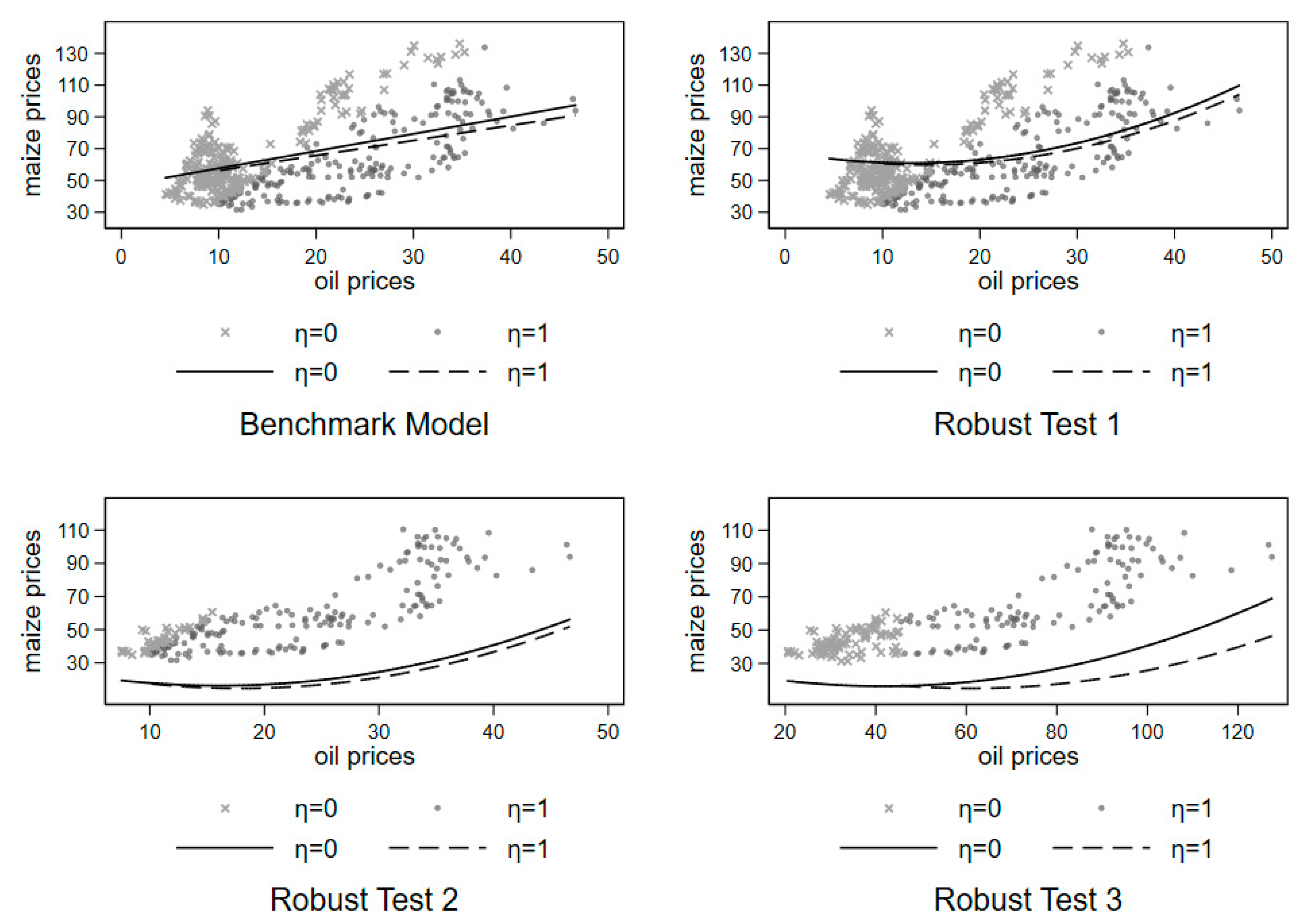
Table 4 for regression (6) to regression (7). When we take a 2nd order Taylor expansion, the threshold value is still 3.7098, and the optimal lead and lag periods of the difference term are 1 and 5. Although, some differences exist in the results of the benchmark model, the overall fitting trend is consistent. In the DFGLS estimation, the coefficients of the cross-term of the indicator and the petroleum price, the indicator, and the constant term are not significant. Another important evidence is the fitting curve (see
Figure 5). The fitting curve with a working demand channel situation is located below the fitting curve without a working demand channel, which is the same as the benchmark results. This means that the development and utilization of bioenergy does not raise maize prices. Therefore, this paper excludes possible bias due to the order of the Taylor series expansion.
The second robustness test is to use partial samples. The points located over or below the ray
represent the different situations of threshold. Points far from the ray have a greater sample-to-sample difference. The differences may be different periods, different prices of oil and maize, and so on. Choosing some points near the ray is important to help determine whether a significant change exists in the influence of the demand channel when only changing the situation of the threshold, i.e., only making the demand channel work or not. Another thought is to choose periods of widespread use of bioenergy. Based on the above two ideas, we choose partial samples with consecutive months. The rule of choosing minimizes the mean differences of two groups of points over or below the ray. A partial sample from July 1999 to June 2017 is reserved. In the optimal 2nd order Taylor series expansion estimation, as shown in regression (8) to regression (9) of
Table 4, coefficients of the cross-term of the indicator and the oil prices, the cross-term of the indicator, and the constant term are still not significant. The fitting curve with a working demand channel situation is located below the fitting curve without the working demand channel (see
Figure 5). These are similar to the results above.
Thirdly, the threshold of empirical data is used to test whether the development of bioenergy will aggravate the rising maize prices. We will completely change the threshold from a maize–oil price ratio to oil prices, which is consistent with the empirical data. Specifically, the oil price data need to be adjusted to a new series, setting January 2007 as the base month. If the new adjusted oil prices are higher than
$45 per barrel, let the indicator
; otherwise, let
. One concern about this series that is too long term is the inability to obtain an accurate price adjustment, so only the data period after January 2000 is reserved in this estimation. The results of estimation of the 2nd order optimal expansion formula are shown in
Table 4 for regression (10) to regression (11). Although one of the coefficients of concern becomes significant, the fitting curve with the working demand channel situation is still located below the fitting curve without working the demand channel (see
Figure 5), thereby providing results consistent with those above.
The fourth one is to use price gaps between maize and wheat and between maize and rice. The correlation between oil prices and food prices is different among the different crop varieties. For example, in the demand channel, maize is the crop most related to oil, with wheat following, and with rice showing the weakest relation of these three crops. Therefore, if the development of bioenergy will aggravate the rising maize prices, when the indicator is above
, the demand channel works, and the price gap between maize and wheat or rice will be significantly reduced. The reason for the reduction is that the prices of rice and wheat are higher than maize, 335.60, 165.46, and 137.62 (dollars per ton) during our observation periods. Data are from IMF. Of course, the impact through the cost channel must be assumed to be similar among these three crops, which is the limitation of the analysis used here. Based on formula (26), the prices gap could be expressed as follows:
where
indicates the gap between the price of wheat or rice and maize. If the coefficients of
and
are negative and significant, it means that the development of bioenergy will raise the maize prices. As shown in
Table 5, the estimated results reject this speculation, which means developing bioenergy would not aggravate maize prices and cause an increase in the long term.
All the empirical analyses confirm the results we obtained with the theoretical analysis. These results suggest that, in the long term, the effect of oil prices on maize prices through demand channels is not very effective, and the production of bioenergy will not significantly increase maize prices. These results are similar to those of some recent related studies such as those of Dillon and Barrett [
15] and Hochman and Zilberman [
16].


