Comparative Analysis between Hydrous Ethanol and Gasoline C Pricing in Brazilian Retail Market

Abstract

The global energy landscape is rapidly changing, including the transition to a low carbon economy and the use of liquid biofuel. The production of liquid biofuel has emerged as an alternative to the use of fossil fuels for purposes of energy conservation, carbon emission mitigation and agricultural development. In this article we study the co-movements between hydrous ethanol and gasoline C in the Brazilian retail market. A multi-scale cross correlation analysis was applied to the Average Retail Margin time series of hydrous ethanol for fifteen relevant retail markets in Brazil to analyze the competitiveness of hydrous ethanol towards gasoline C. The empirical results showed a remarkable different behavior between hydrous ethanol and gasoline C, for any time scale, regardless of geographical distance or regional differences.

1. Introduction

There is a consensus in the scientific community that human activity is related to global warming [1]. The burning of fossil fuels could have severe consequences, for the planet’s environmental balance. Nowadays, the challenges facing by the oil industry is to compete with clean energy sources, which are increasingly present in the world energy matrix. In the last decades discussions about the depletion of natural resources have intensified nations around the world, including the adoption of sustainable energy source, such as renewable energies [2,3].

Although the global community will continue to use fossil fuels during the transition to a low carbon economy, the global energy landscape is changing quickly as predicted by the International Energy Agency [2]. Projections indicate that by 2030 the world’s car fleet will double to 2 billion, most of them still fueled by fossil fuels [4], but the increase of electric cars coupled with fuel efficiency gains should not lead to increased oil consumption for passenger cars. However the demand for oil will continue to grow for trucks, aviation and petrochemicals [2,3].

Bioeconomy may be defined as an economy where materials, chemicals and energy are derived from renewable biological resources [5]. The bioeconomy can adress issues regarding industrial restructuring, energy security and health. Switch from fossil-fuel to bio-fuel, for example, is important from a climate change outlook [6,7].

According to Goldemberg [8], the main example of rapid growth in the use of renewable in developing countries is the sugarcane ethanol program in Brazil. Ethanol is a renewable, domestically produced alcohol fuel made from plant material, such as corn, sugar cane, or grasses. Ethanol is able to mitigate oil dependence and greenhouse gas emissions from cars.

In Brazil, 1975, a relevant initiative aimed at reducing fossil fuel consumption was the Ethanol program for cars, called Pro-Álcool [9]. In the earlier, the program concentrated on production of anhydrous ethanol for blending with gasoline A (Ethanol-free). Now, both products are blended on the distribution companies to form gasoline C. In the 2000’s years, as a reaction to the decreased use of ethanol, the automobile industry started the production of flex fuel light vehicles, that works simultaneously by both ethanol or gasoline C, allowing direct competition between these fuels [10].

In 2011, the Brazilian government implemented Law 12.490 to regulate the biofuel market [11]. This law was created to guarantee the biofuel supply in the country, promote the country’s competitiveness in the international market, attract infrastructure investments and reduce greenhouse gas emissions. It also regulates and authorizes activities related to biofuel production, logistics and facilities, and the assessment and certification of its quality. Currently, the RenovaBio, 2016, is an integrated carbon credit incentive for biofuel [12] just as the United States Renewable Fuel Standard (RFS), the California Low Carbon Fuel Standard (LCFS) and the Renewable Energy Directive (RED) of the European Union [13].

RenovaBio and flex fuel technology initiatives aim to increase ethanol consumption, impacting the Brazilian fuel trade chain (Figure 1) and consequently the final price to the consumer. While Flex Fuel introduced a choice between gasoline C and hydrous ethanol for the final consumer, with a well-established 70% threshold ratio for the relative value of fuels in Brazilian people’s minds [14], RenovaBio may change the current trade chain, by introducing a new direct connection between ethanol plants and service stations [15].

Bioeconomy success may depend on active engagement of policy formulation and specific projects [17]. Despite all Brazilian government policies to promote the use of hydrous ethanol, demand has not kept pace with gasoline C since 2010, as seen in Figure 2. It is related with the current ethanol price and the 70% threshold of gasoline average retail prices. After 2011, policy decisions aimed at stabilizing inflation have strongly contributed to the loss of competitiveness of ethanol [18].

Some studies evaluates the hydrous ethanol as automotive fuel and its relation to the gasoline market regarding the issue of expanding the distribution network in US [19,20,21]. On the other hand, Brazil has a mature ethanol retail market, established since Pro-Álcool. Most studies using Brazilian data explores the convergence of fuels average price toward the law of one price [14,22,23]. Recently, Pessoa et al. [24] evaluated the fuel market in Rio de Janeiro and documented the importance of price dispersion across services stations, arguing that, due the fuel retail market structure in Brazil, price convergence should not necessarily occur.

This paper aims to analyze the inequalities by comparing the co-movements of hydrous ethanol and gasoline C in the Brazilian retail market. The empirical analysis exploits the Average Retail Margin (ARM) for these fuels. By using ARM to analyze the behavior of fuel retail, we leave aside local market variability such as fleet size, logistics and fuel distribution, among others, to assess market performance [25]. For this purpose the coefficient ${\rho }_{DCCA}$ [26] is applied for time series collected from service stations between 2005 and 2014 in fifteen relevant Brazilian cities. The $H_0$ is that the co-movements of hydrous ethanol retail margin are equal to gasoline C.

The structure of this paper is as follows. This section summarizes the Brazilian fuel retail market and the hypotheses of this paper. In Section 2, we explains the data used and the ${\rho }_{DCCA}$ method. In Section 3, we present a detailed discussion regarding the results. Ultimately, we summarize the main points and describe a possible scenario in Section 4.

2. Material and Methods

2.1. Data

To evaluate the hydrous ethanol retail market, the ARM in relevant Brazilian markets [27] was computed. The ARM signal is calculated from $AR{M}_w=r{s}_w-c_w$, where $r{s}_w$ is the average price of hydrous ethanol in the retail market, $c_w$ is the average hydrous ethanol price wholesale, and the index w is weekly, measured over a period that ranges from 2005 to 2014, representing 517 weeks. The original datasets are provided by Agência Nacional do Petróleo, Gás Natural e Biocombustíveis (ANP) [12]. The

Table 1. Regions, cities and location (latitude and longitude).

Region	City	Latitude, Longitude
North	Belém (BEL)	−1.382051, −48.477898
	Manaus (MAO)	−3.036105, −60.046593
	Rio Branco (RBR)	−9.866168, −67.897189
Northeast	Fortaleza (FOR)	−3.777554, −38.533172
	Recife REC)	−8.061129, −34.871665
	Salvador (SSA)	−12.911014, −38.331413
Central−West	Brasília (BSB)	−15.869923, −47.917428
	Cuiabá (CGB)	−15.594821, −56.091696
	Goiânia (GYN)	−16.601095, −49.144543
Southeast	Belo Horizonte (BHZ)	−19.846098, −43.963296
	Rio de Janeiro (RIO)	−22.913002, −43.180002
	São Paulo (SAO)	−23.589592, −46.660721
South	Curitiba (CWB)	−25.442395, −49.240417
	Florianópolis (FLN)	−27.670175, −48.545944
	Porto Alegre (POA)	−29.993399, −51.175563

shows the fifteen relevant markets evaluated as well as their coordinates.

The second dataset were obtained from [25], where the DCCA cross-correlation coefficients for the gasoline C retail market have been calculated in the same period of time, for identical pairs and using the model presented in Section 2.2.

2.2. Statistical Model

A well established method to assess cross-correlation between two different time series is the Spearman’s coefficient [28]. Lately, other methods were developed to address the evaluation of dynamic systems, like Detrending Moving-Average coefficient [29] and DCCA cross-correlation coefficient [30], to measure linear and non-linear cross-correlation of non-stationary time series [31,32,33]. DCCA cross-correlation coefficient [30] is based on the autocorrelation studies in time series [34] and the evaluation of cross-correlation between time series by power law [35]. The ${\rho }_{DCCA}$ coefficient is able to estimate the value of cross-correlation between two time series in various time scales.

Several studies have used the ${\rho }_{DCCA}$ coefficient, their applications including cross-correlation between the largest companies assets blue chips in the Brazilian stock exchange and between the G-7 countries, studying the periods before and after the 2008 crisis and finding a substantial increase in the post-crisis period [36,37]. Ferreira and Pereira [38] evaluated the price of crude oil to twenty stock exchanges before and after the crisis of 2008. Kristoufek [29] applied the detrending and moving-average cross-correlation coefficient in energy commodities testing the leverage effect. In Energy Finance, Wang et al. [39] calculated coefficients to quantify the cross-correlations between energy and emission markets.

It was also used to study the political and financial implications of Brexit [38]; the use of ${\rho }_{DCCA}$ coefficient working together with network analysis in the US stock market [40], combining the two matrices with the Random Matrix Theory method to assess the cross correlations in the US stock market. Other applications involving finances are from [41,42,43,44,45,46]. Recently, a variation was introduced for calculation of the Detrended Multiple Cross Correlation Coefficient [26]). According to Pereira et al. [47], the use of complex systems tools in economics is named econophysics, including the multiscale cross-correlation method [48,49,50]. Some other papers have evolved the application of cross-correlation methods, like Kwapień et al. [31], Qian et al. [32], Kristoufek [29], Jiang et al. [51], Kristoufek [52], Wang et al. [53], Yuan et al. [54] and Wang et al. [55].

The ${\rho }_{DCCA}$ is calculated as follow:

• Integrate two time series, $\left\{x_t\right\}$ and $\left\{y_t\right\}$, to generate two new series $x{x}_k={\sum }_{t=1}^k{x}_t$ and $y{y}_k={\sum }_{t=1}^k{y}_t,k=1,2,\dots ,N$, where N is number of elements of the time series.
• Divide $\left\{x{x}_k\right\}$ and $\left\{y{y}_k\right\}$ in $\left(N-s\right)$ overlapping boxes of equal length s, with $4\le s\le \frac{N}{4}$.
• The least squares adjustment of each time series calculates the local trend of each box, $x{P}_i\left(k\right)$ and $y{P}_i\left(k\right)$. The covariance of the residuals is calculated by Equation (1):

  $$f^2{}_{xy}\left(s,i\right)=\frac{1}{s+1}\sum _{k=1}^{i+s}(x{x}_k-x{P}_i\left(k\right))(y{y}_k-y{P}_i\left(k\right)).$$

  (1)
• The new covariance function (Equation (2)):

  $$F^2{}_{xy}\left(s\right)=\frac{1}{N-s}\sum _{i=1}^{N-s}{f}^2{}_{xy}\left(s,i\right).$$

  (2)
• The ${\rho }_{DCCA}$ is (Equation (3)):

  $${\rho }_{DCCA}\left(s\right)=\frac{F^2{}_{xy}\left(s\right)}{F_{xx}\left(s\right)F_{yy}\left(s\right)}.$$

  (3)

The $F^2{}_{xy}\left(s\right)$ is the correlation function (Podobnik and Stanley [35]). $F_{xx}\left(s\right)$ and $F_{yy}\left(s\right)$ are the autocorrelation functions (Peng et al. [34]). ${\rho }_{DCCA}$ is a dimensionless coefficient that measures cross-correlation, ranging from 1 to $-1$ [56].

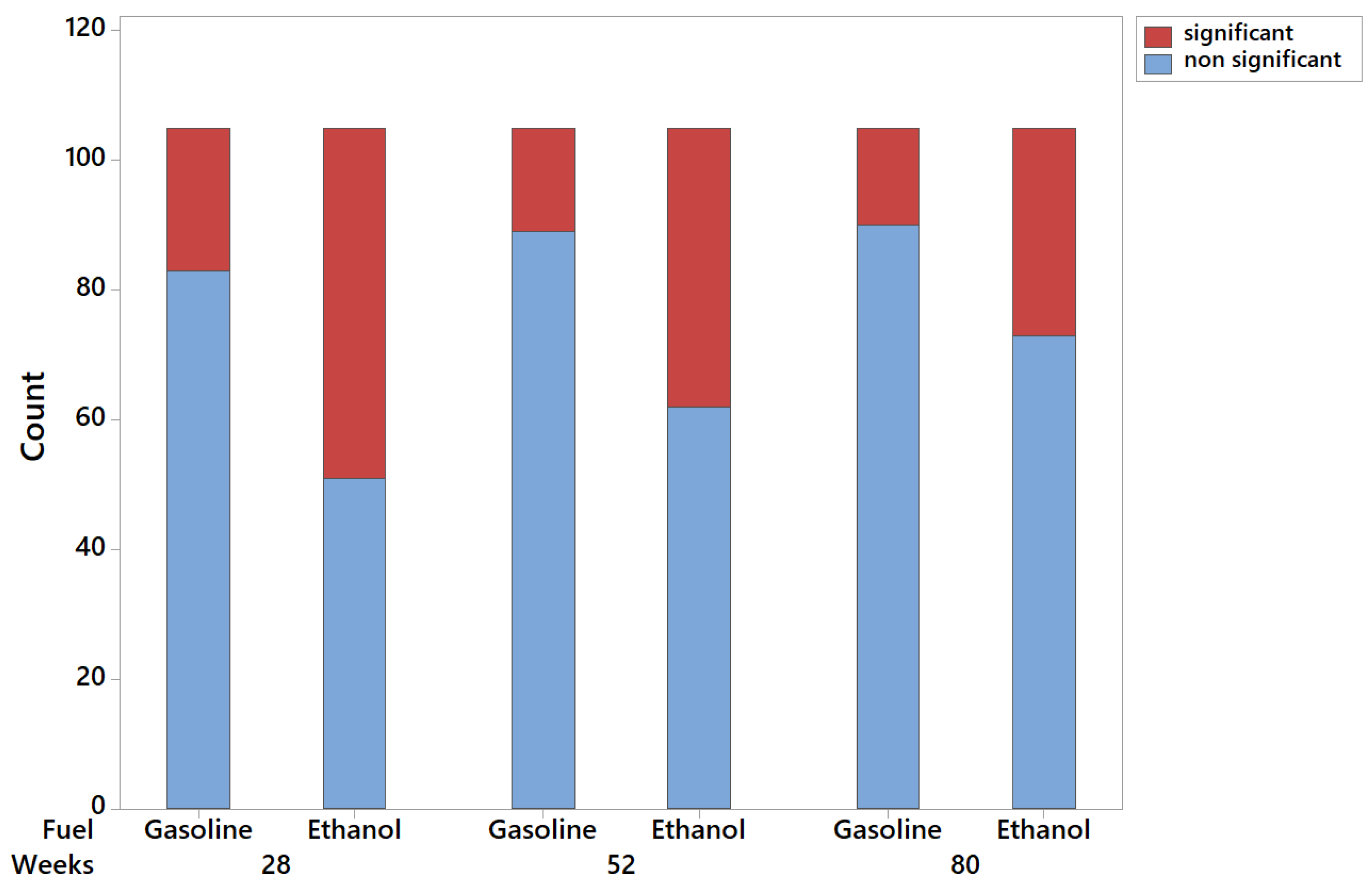
3. Results and Discussion

Analysis of the hydrous ethanol results will take into consideration the statistical test of Podobnik et al. [57]. The correlation is statistically significant if is outside the lower and upper limits, with significance of 95%, for the hypothesis test of H0: ${\rho }_{DCCA}=0$ and H1: ${\rho }_{DCCA}\ne 0$. For instance, the LL95% and UL95% inside the graphs are the significant levels calculated and represent the lower and upper limits, respectively.

Only for viewing and analyzing purposes, any presented results on Section 3 are based on city pairs that reach, for any time scale, medium or strong cross-correlations coefficients according to the suggested intervals by Zebende et al. [26] and statistically significant.

All cities from the South and Southeast presented significant ARM coefficients, highlighting BHZ-RIO, which reached a ${\rho }_{DCCA}$ of $0.79$, the highest correlation value of the whole assessment, and the only one within the strong cross-correlation interval (Figure 3). Highlighted is the city of BHZ, remaining significantly cross-correlated with all the cities from the South (FLN, POA and CWB) and Southeast (RIO and SAO) of Brazil for 95% or more of the time scale boxes.

In fewer pairs than in the south-southeast, some of the North and Northeast cities are medium cross-correlated (Figure 4). SSA, for example, is correlated only with RBR in the region, located over 3200 km away. SSA has a very weak cross-correlation with the nearest cities in the Northeast, smaller than a ${\rho }_{DCCA}$ of $0.20$ for REC and $0.17$ for FOR.

A finding to be highlighted is the cross-correlation between MAO-POA, reaching the medium condition interval (${\rho }_{DCCA}$ of 0.59 for 60 weeks) and remaining always significant. POA, in the South, is more than 3100 Km away from MOA, considering a linear distance measurement (LDM), in the North of Brazil (Figure 5).

Another finding that deserves attention is the pair FOR-RIO, which reaches a ${\rho }_{DCCA}$ maximum of 0.42 and the cross-correlations values are significant for all time scale box. RIO was also cross-correlated with BEL (BEL-RIO), with a ${\rho }_{DCCA}$ maximum of 0.52 for 52 weeks. RIO is more than 2100 Km LDM away from FOR and 2400 Km LDM from BEL (Figure 5).

Pairs GYN-SAO, CGB-RBR and BEL-GYN presented a medium cross-correlation condition in at least one time scale and are significantly positive. GYN and CGB are located in the Central-West of Brazil, and they were correlated with cities from the Southeast and North (Figure 6), but not with each other. CGB-RBR is significantly cross-correlated for 85% of the time scale. Pairs CGB-SAO, CGB-GYN, GYN-SSA, CGB-CWB, CGB-MAO and GYN-RBR presented an anti-correlated behaviour for some time scale (Figure 7).

Comparison between Hydrous Ethanol and Gasoline C Retail Markets

According to [25], SAO seems to exert control on BHZ and RIO ARM in the gasoline C retail market. Furthermore, most coefficients for gasoline C were not significant. Only the pairs BHZ-RIO, BHZ-SAO, RIO-SAO, RBR-SSA, FLN-GYM, BSB-GYM, CGB-FOR, CGB-REC, FOR-REC, BSB-FLN, CWB-SAO, BSB-CWB, BSB-RBR, CWB-RBR, GYM-REC, GYM-RIO, CGB-SAO, CGB-RIO, MAO-RBR, FLN-FOR, BEL-CGB, FOR-MAO, BEL-FOR and BSB-FOR presented a ${\rho }_{DCCA}$ greater than $0.33$ for any of the calculated time scales.

Figure 8 shows a summary of gasoline C and hydrous ethanol results, were the percentiles where calculated based on the statistical test of [57]. This summary was created for three time scale periods: 28, 52 and 80 weeks. This decision was based on the sugar cane varieties production cycles. In Brazil, the plant’s cane harvests are typically 12 or 18 months [58].

The difference in the amount of significant cross-correlations found between fuels is huge. For instance, there is 79% of non-significant cross-correlations for gasoline C, against 48.6% for hydrous ethanol in 28 weeks. The significant cross-correlation coefficient percentile remains visually stable for 28, 52 and 80 weeks on the gasoline C summary.

The city of POA was chosen to demonstrate the differences between the gasoline C and hydrous ethanol retail market. Cross-correlation coefficient of pairs BHZ-POA, FLN-POA, MAO-POA, POA-RIO and POA-SAO reached more than $0.33$ for hydrous ethanol, but never exceeded it for the gasoline C market, in any time scale (Figure 9).

4. Conclusions

The empirical results rejected the hypothesis that the co-movements of hydrous ethanol ARM are equal to gasoline C. Results also showed a remarkable different behavior between hydrous ethanol and gasoline C in Brazilian retail market co-movements, from the statistical point of view. There is a decrease of non significant coefficients in hydrous ethanol compared with gasoline C, 48.6% and 79.1% respectively, for the 28-week time scale. Since the ARM emerges from the fuel price decided in each service station, it means a reduction in the competitiveness of the price of ethanol, identified in the increase in non-random movements between the cities.

For instance, the pair MAO-POA, more than 3100 Km from each other, reached a ${\rho }_{DCCA}$ of 0.59 for 60 weeks with hydrous ethanol, representing a highly significant interdependent market. Manaus has a Human Development Index (HDI) of 0.737, ranked at ${867}^{\circ }$ in Brazil and Porto Alegre has a HDI of 0.805, ranked at ${33}^{\circ }$, in the 2010 Human Development Report. Manaus’s Gross Domestic Product per capita is $R\$$33,564.11, while in Porto Alegre is $R\$$49,577.53 [59], indicating significant differences between the cities‘ economies.

Although the Brazilian government invests heavily in incentive policies in the biofuel production and distribution chain, a lack of competitiveness between hydrous ethanol and gasoline C over the year is observed in Figure 2, due to the loss of hydrous ethanol market share over the years. In order to minimize that, one suggestion would be promote “biofuel only” service stations, through Renovabio carbon credit incentives, to make hydrous ethanol a perfect substitute for gasoline C. Hence, in a near future, other biofuels used around the world, like Biodiesel B100, would take advantage of this new retail structure.

DCCA Cross-correlation coefficient may be an efficient tool to identify price co-movements in any complex fuel retail market. The method can be used by ANP to create a fuel market intelligence computer model, enabling new ways of assessing retail competition to identify indications of cartel or tacit collusion.

References

1. Cook, J.; Oreskes, N.; Doran, P.T.; Anderegg, W.R.; Verheggen, B.; Maibach, E.W.; Carlton, J.S.; Lewandowsky, S.; Skuce, A.G.; Green, S.A.; et al. Consensus on consensus: A synthesis of consensus estimates on human-caused global warming. Environ. Res. Lett. 2016, 11, 048002. [Google Scholar] [CrossRef]
2. Conti, J.; Holtberg, P.; Diefenderfer, J.; LaRose, A.; Turnure, J.T.; Westfall, L. International Energy Outlook 2016 with Projections to 2040; Technical Report DOE/EIA-0484; USDOE Energy Information Administration (EIA), Office of Energy Analysis: Washington, DC, USA, 2016.
3. Cook, J.; Nuccitelli, D.; Green, S.A.; Richardson, M.; Winkler, B.; Painting, R.; Way, R.; Jacobs, P.; Skuce, A. Quantifying the consensus on anthropogenic global warming in the scientific literature. Environ. Res. Lett. 2013, 8, 024024. [Google Scholar] [CrossRef] [Green Version]
4. Gross, M. Planet with two billion cars. Curr. Biol. 2016, 26, 307–410. [Google Scholar] [CrossRef]
5. Directorate-General for Research and Innovation (European Commission). Innovating for Sustainable Growth: A Bioeconomy for Europe; Publications Office of the European Union: Luxembourg, 2012. [Google Scholar] [CrossRef]
6. Ollikainen, M. Forestry in bioeconomy—Smart green growth for the humankind. Scand. J. For. Res. 2014, 29, 360–366. [Google Scholar] [CrossRef]
7. Richardson, B. From a fossil-fuel to a biobased economy: The politics of industrial biotechnology. Environ. Plan. C Gov. Policy 2012, 30, 282–296. [Google Scholar] [CrossRef]
8. Goldemberg, J. Ethanol for a sustainable energy future. Science 2007, 315, 808–810. [Google Scholar] [CrossRef] [PubMed]
9. Brazil. Decree n. 76593 de 14 de Novembro de 1975. Diário Oficial, 1975. Available online: https://www2.camara.leg.br/legin/fed/decret/1970-1979/decreto-76593-14-novembro-1975-425253-norma-pe.html (accessed on 5 April 2019).
10. Kamimura, A.; Sauer, I.L. The effect of flex fuel vehicles in the Brazilian light road transportation. Energy Policy 2008, 36, 1574–1576. [Google Scholar] [CrossRef]
11. Brazil. Law n. 12940 de 16 de Setembro de 2011. Diário Oficial, 2011. Available online: http://www.planalto.gov.br/ccivil_03/_Ato2011-2014/2011/Lei/L12490.htm (accessed on 5 April 2019).
12. ANP. Agência Nacional do Petróleo, Gás Natural e Biocombustíveis. 2019. Available online: http://www.anp.gov.br (accessed on 5 April 2019).
13. Delgado, F.; Sousa, M.E.d.; Roitman, T. Biocombustíveis. Cad. De Biocombustíveis 2017, 4, 21–23. [Google Scholar]
14. Salvo, A.; Huse, C. Is arbitrage tying the price of ethanol to that of gasoline? Evidence from the uptake of flexible-fuel technology. Energy J. 2011, 119–148. [Google Scholar] [CrossRef]
15. ANP. Agência Nacional do Petróleo, Gás Natural e Biocombustíveis. Available online: http://www.anp.gov.br/images/Consultas_publicas/2018/TPC/TPC2-2018/NT_GT_TPC2_2018.pdf (accessed on 5 April 2019).
16. Petrobras. Gasoline. Available online: http://www.petrobras.com.br/en/products-and-services/composition -of-sales-prices-to-the-consumer/gasoline/ (accessed on 12 May 2019).
17. McCormick, K.; Kautto, N. The bioeconomy in Europe: An overview. Sustainability 2013, 5, 2589–2608. [Google Scholar] [CrossRef]
18. EPE—Empresa de Pesquisa Energética. Análise de Conjuntura dos Biocombustíveis. 2017. Available online: http://www.mme.gov.br (accessed on 12 May 2019).
19. Anderson, S.T. The demand for ethanol as a gasoline substitute. J. Environ. Econ. Manag. 2012, 63, 151–168. [Google Scholar] [CrossRef]
20. Corts, K.S. Building out alternative fuel retail infrastructure: Government fleet spillovers in E85. J. Environ. Econ. Manag. 2010, 59, 219–234. [Google Scholar] [CrossRef] [Green Version]
21. Shriver, S.K. Network effects in alternative fuel adoption: Empirical analysis of the market for ethanol. Mark. Sci. 2015, 34, 78–97. [Google Scholar] [CrossRef]
22. Boff, H.P. Modeling the Brazilian ethanol market: How flex-fuel vehicles are shaping the long run equilibrium. China-USA Bus. Rev. 2011, 10, 245–264. [Google Scholar]
23. Ferreira, A.L.; de Almeida Prado, F.P.; da Silveira, J.J. Flex cars and the alcohol price. Energy Econ. 2009, 31, 382–394. [Google Scholar] [CrossRef]
24. Pessoa, J.P.; Rezende, L.; Assunção, J. Flex cars and competition in fuel retail markets. Int. J. Ind. Organ. 2019, 63, 145–184. [Google Scholar] [CrossRef]
25. Nascimento Filho, A.; Pereira, E.; Ferreira, P.; Murari, T.; Moret, M. Cross-correlation analysis on Brazilian gasoline retail market. Phys. A Stat. Mech. Appl. 2018, 508, 550–557. [Google Scholar] [CrossRef]
26. Zebende, G.; Brito, A.; Silva Filho, A.; Castro, A. ρDCCA applied between air temperature and relative humidity: An hour/hour view. Phys. A Stat. Mech. Appl. 2018, 494, 17–26. [Google Scholar] [CrossRef]
27. Pedra, D.P.; de Oliveira Bicalho, L.M.N.; de Araújo Vilela, O.; Baran, P.H.; de Paiva, R.M.; de Melo, T.P. Metodologia Adotada pela Agência Nacional do Petróleo, Gás Natural e Biocombustíveis para a Detecção de Cartéis. 2010. Available online: http://www.anp.gov.br (accessed on 12 May 2019).
28. Spearman, C. The proof and measurement of association between two things. Am. J. Psychol. 1904, 15, 72–101. [Google Scholar] [CrossRef]
29. Kristoufek, L. Detrending moving-average cross-correlation coefficient: Measuring cross-correlations between non-stationary series. Phys. A Stat. Mech. Appl. 2014, 406, 169–175. [Google Scholar] [CrossRef] [Green Version]
30. Zebende, G. DCCA cross-correlation coefficient: Quantifying level of cross-correlation. Phys. A Stat. Mech. Appl. 2011, 390, 614–618. [Google Scholar] [CrossRef]
31. Kwapień, J.; Oświkecimka, P.; Drożdż, S. Detrended fluctuation analysis made flexible to detect range of cross-correlated fluctuations. Phys. Rev. E 2015, 92, 052815. [Google Scholar] [CrossRef] [PubMed] [Green Version]
32. Qian, X.Y.; Liu, Y.M.; Jiang, Z.Q.; Podobnik, B.; Zhou, W.X.; Stanley, H.E. Detrended partial cross-correlation analysis of two nonstationary time series influenced by common external forces. Phys. Rev. E 2015, 91, 062816. [Google Scholar] [CrossRef] [PubMed] [Green Version]
33. Zhao, X.; Shang, P.; Huang, J. Several fundamental properties of DCCA cross-correlation coefficient. Fractals 2017, 25, 1750017. [Google Scholar] [CrossRef]
34. Peng, C.K.; Buldyrev, S.V.; Havlin, S.; Simons, M.; Stanley, H.E.; Goldberger, A.L. Mosaic organization of DNA nucleotides. Phys. Rev. E 1994, 49, 1685. [Google Scholar] [CrossRef] [PubMed]
35. Podobnik, B.; Stanley, H.E. Detrended cross-correlation analysis: A new method for analyzing two nonstationary time series. Phys. Rev. Lett. 2008, 100, 084102. [Google Scholar] [CrossRef] [PubMed]
36. da Silva, M.F.; Pereira, É.J.d.A.L.; da Silva Filho, A.M.; de Castro, A.P.N.; Miranda, J.G.V.; Zebende, G.F. Quantifying cross-correlation between Ibovespa and Brazilian blue-chips: The DCCA approach. Phys. A Stat. Mech. Appl. 2015, 424, 124–129. [Google Scholar] [CrossRef]
37. da Silva, M.F.; Pereira, É.J.d.A.L.; da Silva Filho, A.M.; de Castro, A.P.N.; Miranda, J.G.V.; Zebende, G.F. Quantifying the contagion effect of the 2008 financial crisis between the G7 countries (by GDP nominal). Phys. A Stat. Mech. Appl. 2016, 453, 1–8. [Google Scholar] [CrossRef]
38. Ferreira, P.; Pereira, É. The impact of the Brexit referendum on British and European Union bank shares: A cross-correlation analysis with national indices. Econ. Bull. 2019, 39, 335–346. [Google Scholar]
39. Wang, G.J.; Xie, C.; Chen, S.; Han, F. Cross-correlations between energy and emissions markets: New evidence from fractal and multifractal analysis. Math. Probl. Eng. 2014, 2014, 197069. [Google Scholar] [CrossRef]
40. Wang, G.J.; Xie, C.; Chen, S.; Yang, J.J.; Yang, M.Y. Random matrix theory analysis of cross-correlations in the US stock market: Evidence from Pearson’s correlation coefficient and detrended cross-correlation coefficient. Phys. A Stat. Mech. Appl. 2013, 392, 3715–3730. [Google Scholar] [CrossRef]
41. Ferreira, P.; Dionisio, A. Revisiting covered interest parity in the European Union: The DCCA Approach. Int. Econ. J. 2015, 29, 597–615. [Google Scholar] [CrossRef]
42. Ferreira, P.; Kristoufek, L. What is new about covered interest parity condition in the European Union? Evidence from fractal cross-correlation regressions. Phys. A Stat. Mech. Appl. 2017, 486, 554–566. [Google Scholar] [CrossRef]
43. Da Silva, M.; da Silva Filho, A.; de Castro, A.N. Quantificando a Influência do Mercado de Câmbio nos Preços do Milho e da Soja no Município de Barreiras. Conjunt. Planej 2014, 182, 45–51. [Google Scholar]
44. Bashir, U.; Zebende, G.F.; Yu, Y.; Hussain, M.; Ali, A.; Abbas, G. Differential market reactions to pre and post Brexit referendum. Phys. A Stat. Mech. Appl. 2019, 515, 151–158. [Google Scholar] [CrossRef]
45. Guedes, E.; Dionisio, A.; Ferreira, P.; Zebende, G. DCCA cross-correlation in blue-chips companies: A view of the 2008 financial crisis in the Eurozone. Phys. A Stat. Mech. Appl. 2017, 479, 38–47. [Google Scholar] [CrossRef]
46. Hussain, M.; Zebende, G.F.; Bashir, U.; Donghong, D. Oil price and exchange rate co-movements in Asian countries: Detrended cross-correlation approach. Phys. A Stat. Mech. Appl. 2017, 465, 338–346. [Google Scholar] [CrossRef]
47. Pereira, E.J.d.A.L.; da Silva, M.F.; Pereira, H.d.B. Econophysics: Past and present. Phys. A Stat. Mech. Appl. 2017, 473, 251–261. [Google Scholar] [CrossRef]
48. Stanley, H.E.; Afanasyev, V.; Amaral, L.A.N.; Buldyrev, S.; Goldberger, A.; Havlin, S.; Leschhorn, H.; Maass, P.; Mantegna, R.N.; Peng, C.K.; et al. Anomalous fluctuations in the dynamics of complex systems: From DNA and physiology to econophysics. Phys. A Stat. Mech. Appl. 1996, 224, 302–321. [Google Scholar] [CrossRef]
49. Mantegna, R.N.; Stanley, H.E. An Introduction to Econophysics: Correlation and Complexity in Finance; Cambridge University Press: Cambridge, UK, 2000; Volume 1. [Google Scholar]
50. Mantegna, R.N.; Stanley, H.E. Scaling behaviour in the dynamics of an economic index. Nature 1995, 376, 46–49. [Google Scholar] [CrossRef]
51. Jiang, Z.Q.; Zhou, W.X. Multifractal detrending moving-average cross-correlation analysis. Phys. Rev. E 2011, 84, 016106. [Google Scholar] [CrossRef] [PubMed] [Green Version]
52. Kristoufek, L. Measuring correlations between non-stationary series with DCCA coefficient. Phys. A Stat. Mech. Appl. 2014, 402, 291–298. [Google Scholar] [CrossRef] [Green Version]
53. Wang, G.J.; Xie, C.; He, L.Y.; Chen, S. Detrended minimum-variance hedge ratio: A new method for hedge ratio at different time scales. Phys. A Stat. Mech. Appl. 2014, 405, 70–79. [Google Scholar] [CrossRef]
54. Yuan, N.; Xoplaki, E.; Zhu, C.; Luterbacher, J. A novel way to detect correlations on multi-time scales, with temporal evolution and for multi-variables. Sci. Rep. 2016, 6, 27707. [Google Scholar] [CrossRef] [PubMed] [Green Version]
55. Wang, G.J.; Xie, C.; Lin, M.; Stanley, H.E. Stock market contagion during the global financial crisis: A multiscale approach. Financ. Res. Lett. 2017, 22, 163–168. [Google Scholar] [CrossRef]
56. Machado Filho, A.; Da Silva, M.; Zebende, G. Autocorrelation and cross-correlation in time series of homicide and attempted homicide. Phys. A Stat. Mech. Appl. 2014, 400, 12–19. [Google Scholar] [CrossRef] [Green Version]
57. Podobnik, B.; Jiang, Z.Q.; Zhou, W.X.; Stanley, H.E. Statistical tests for power-law cross-correlated processes. Phys. Rev. E 2011, 84, 066118. [Google Scholar] [CrossRef] [PubMed] [Green Version]
58. Macedo, I.; Leal, M.; Silva, J. Assessment of Greenhouse Gas Emissions in the Production and Use of Fuel Ethanol in Brazil. 2004. Available online: https://gssd.mit.edu/search-gssd/site/assessment -greenhouse-gas-emissions-60988-mon-11-16-2015-1124 (accessed on 5 April 2019).
59. IBGE. Índice de Desenvolvimento Humano. Available online: https://cidades.ibge.gov.br (accessed on 10 May 2019).
Figure 1. Brazilian trade chain for hydrous ethanol and gasoline C [16]. Any fuel sold to the final consumer and fleet goes through the distribution companies, responsible for blending anhydrous ethanol and gasoline A to formulate gasoline C. Both fuels are sold by the same firm (service stations) in Brazil.
Sustainability 11 04719 g001
Figure 2. Annual demand for hydrous ethanol and gasoline C [18]. Hydrous ethanol demand has not kept pace with gasoline C since 2010.
Sustainability 11 04719 g002
Figure 3. Cross-correlation results for all time scales of the South and Southeast pairs BHZ-RIO, RIO-SAO, BHZ-SAO, FLN-POA, CWB-FLN, FLN-SAO, BHZ-FLN, BHZ-POA, POA-RIO, CWB-SAO, POA-SAO, FLN-RIO, BHZ-CWB and CWB-RIO. The value of the ρ D C C A between BHZ and RIO exceeds 0.66 already with eleven weeks of time scale and remains strong up to 80 weeks.
Sustainability 11 04719 g003
Figure 4. Cross-correlation results of the North and Northeast pairs FOR-REC, BEL-RBR, MAO-RBR, BEL-MAO, BEL-FOR, RBR-SSA, MAO-REC and RBR-REC for all time scales. FOR-REC, BEL-MAO and BEL-FOR are significantly cross-correlated for more than 95% of the time scale.
Sustainability 11 04719 g004
Figure 5. Cross-correlation results of the pairs FLN-FOR, FOR-RIO, BHZ-REC, MAO-POA, CWB-MAO, BEL-RIO, BHZ-MAO, BEL-BHZ, MAO-RIO, showing all cities from North or Northeast whose coefficient reached the medium interval with cities from South or Southeast, for any time scale.
Sustainability 11 04719 g005
Figure 6. Cross-correlation results of the pairs GYN-SAO, CGB-RBR and BEL-GYN for all time scales. No cross-correlation was found between the cities of the Central-West.
Sustainability 11 04719 g006
Figure 7. Cross-correlation results of the pairs CGB-SAO, CGB-GYN, GYN-SSA, CGB-CWB, GYN-RBR and CGB-MAO, significantly negative, for any time scale.
Sustainability 11 04719 g007
Figure 8. Gasoline C and hydrous ethanol summary of ρ D C C A coefficients for all pairs in 28, 52 and 80-week time scale boxes. The bars present significant (red) and non significant (blue) absolute count for both fuels. We highlight that in 28 weeks there is 79% of non-significant cross-correlations for gasoline C, against 48.6% for hydrous ethanol.
Sustainability 11 04719 g008
Figure 9. Cross-correlation results of the pairs BHZ-POA, FLN-POA, MAO-POA, POA-RIO and POA-SAO, for hydrous ethanol (E) and gasoline C (G). Hydrous ethanol DCCA cross-correlation coefficients reaches more than 0.33 from 28 to 80 weeks, but gasoline C never reaches this interval.
Sustainability 11 04719 g009