Charging Network Planning for Electric Bus Cities: A Case Study of Shenzhen, China


Abstract
1. Introduction
1.1. 100% Electric Bus City
1.2. Large-Scale E-Bus Charging Station Solution
- Compared with other vehicle types, buses have strict operation tasks and their charging demand is rigid. The charging demand must be fulfilled at the time when needed, otherwise passenger transport tasks will be influenced, which is not permissible for bus operation. To eliminate the level of disturbance from personal EVs and taxies, bus charging stations are better to be appropriative.
- In the case of public charging stations, these mainly serve small-size vehicles; therefore, the area of the charging spots is not usually large enough to accommodate buses, whose lengths can reach 9 to 12 m.
- Since e-bus battery sizes are large and e-buses have operation tasks, a high charging speed is usually used to decrease charging time as the charging time takes away from the bus operation time. The designed charging rate for public charging stations may not meet the charging requirement of e-buses.
1.3. E-Bus Charging Infrastructure Planning
1.4. Grid Consideration
- (1)
- The work specifically targeted large-scale plug-in charging station planning for e-buses according to bus operation characteristics. Since the operation mode of buses is significantly different from that of private cars and taxis, it was of merit to carry out the planning for bus charging stations.
- (2)
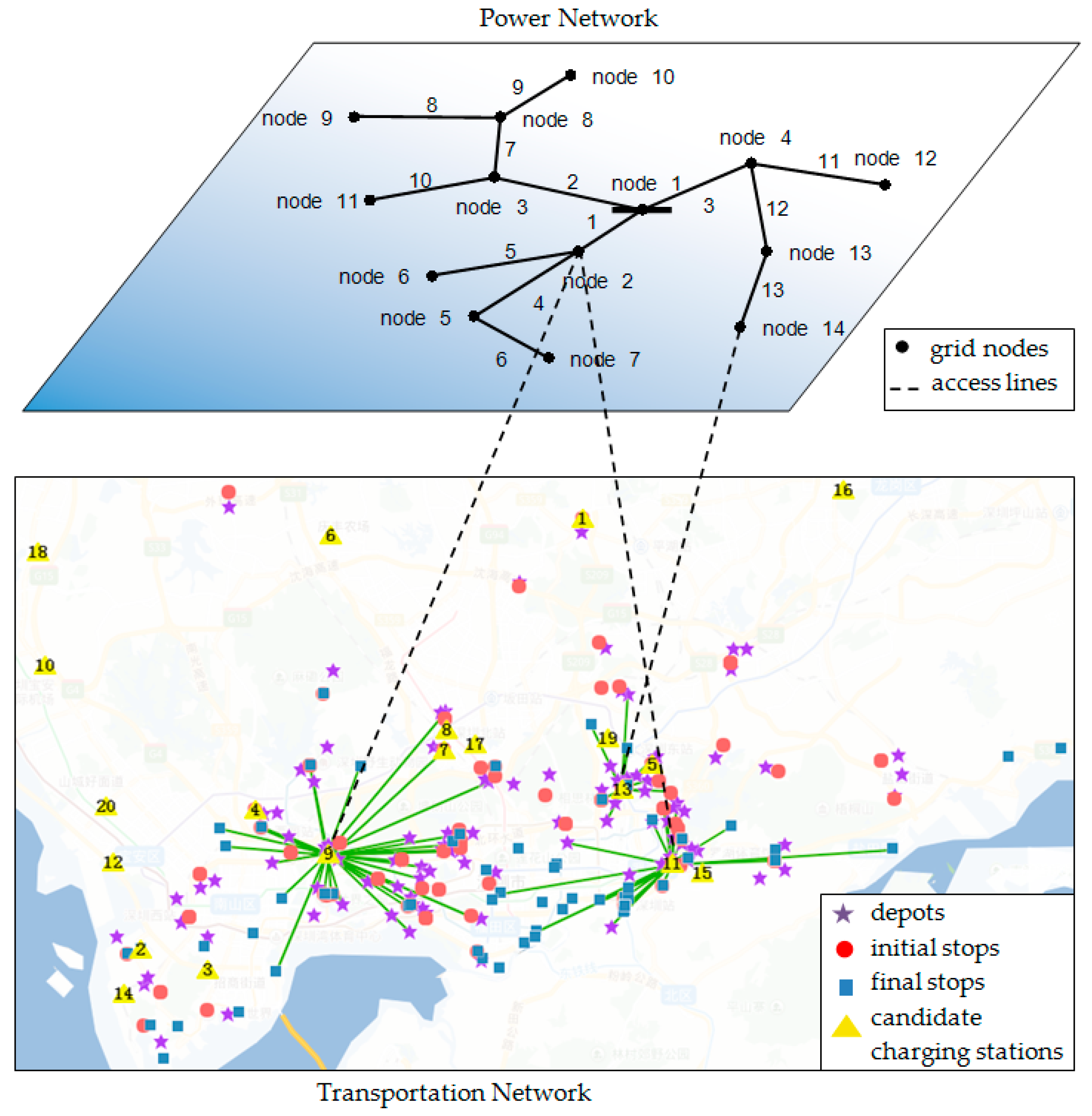
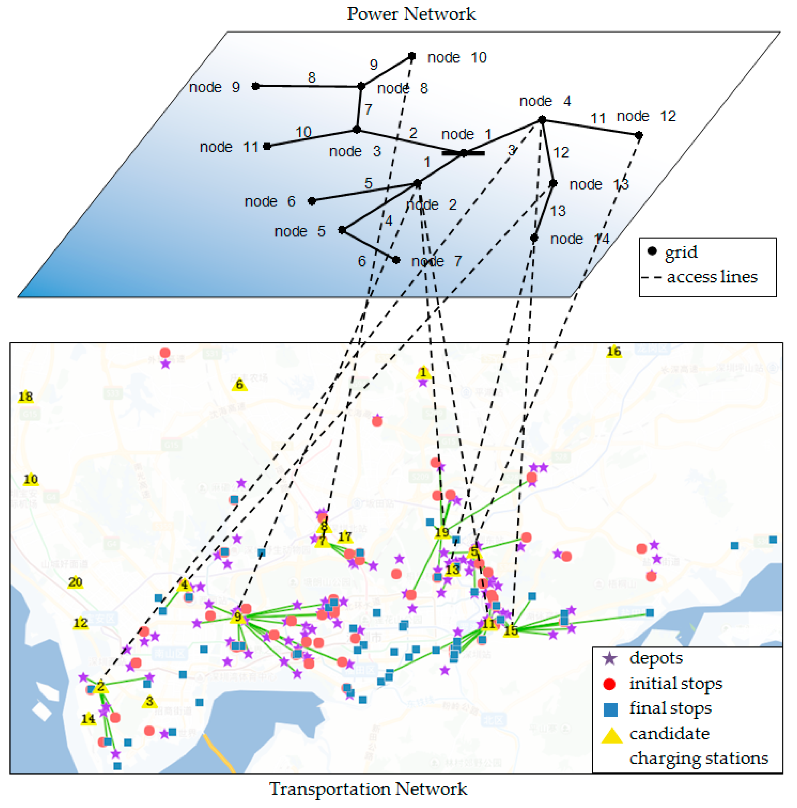
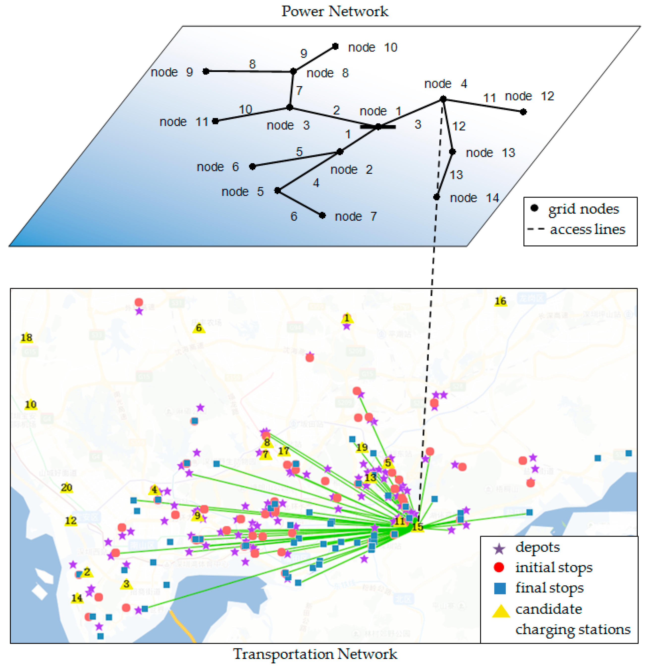
- Conduct interdisciplinary research to combine the transportation network with the power grid into the model to achieve the global optimization of the two systems.
- (3)
- Transform the model into mixed-integer second-order cone programming (MISOCP) and further propose a “No R” exact algorithm to improve the computational speed.
- (4)
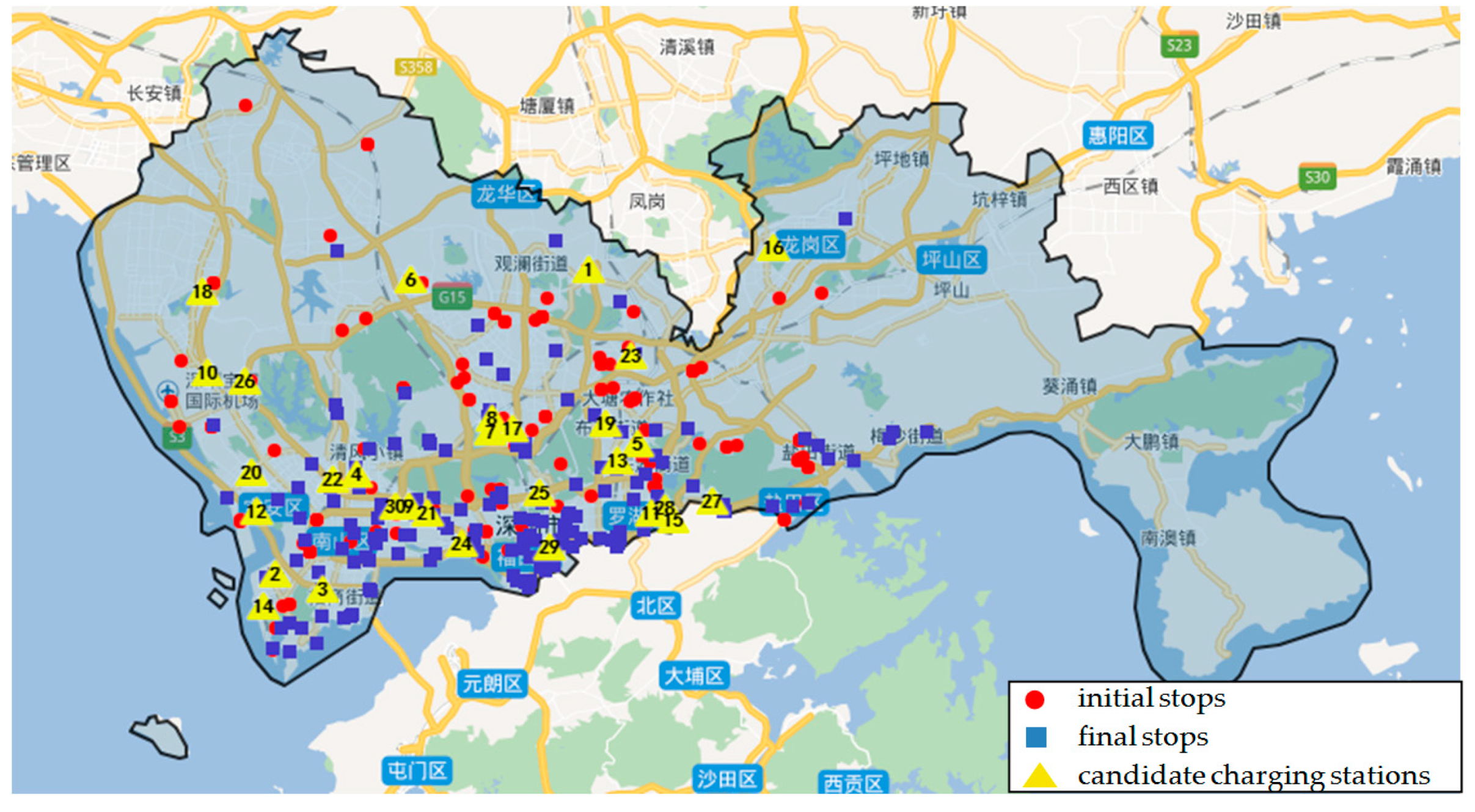
- Implement a case study of the real-world transportation network in Shenzhen and study the impacts of EV technology advancements on the cost and the infrastructure layout. One major finding was that the e-bus driving range is the key factor to lower the cost of the bus charging system.
2. Large-Scale Charging Station Planning Model for Electric Buses
2.1. E-Bus Charging Characteristics
2.2. The Planning Model
3. Solution Method
3.1. Mixed-Integer Second-Order Cone Programming (MISOCP)
3.2. Improved MISOCP
4. Computational Studies
4.1. Numerical Experiments
4.1.1. Joint Optimization
4.1.2. Joint Optimization vs. Separate Optimization

- Step 1. Use Part 2 as the objective function to optimize the power system.
- Step 2. Calculate Part 1.
4.1.3. Comparison
4.2. Technological Considerations
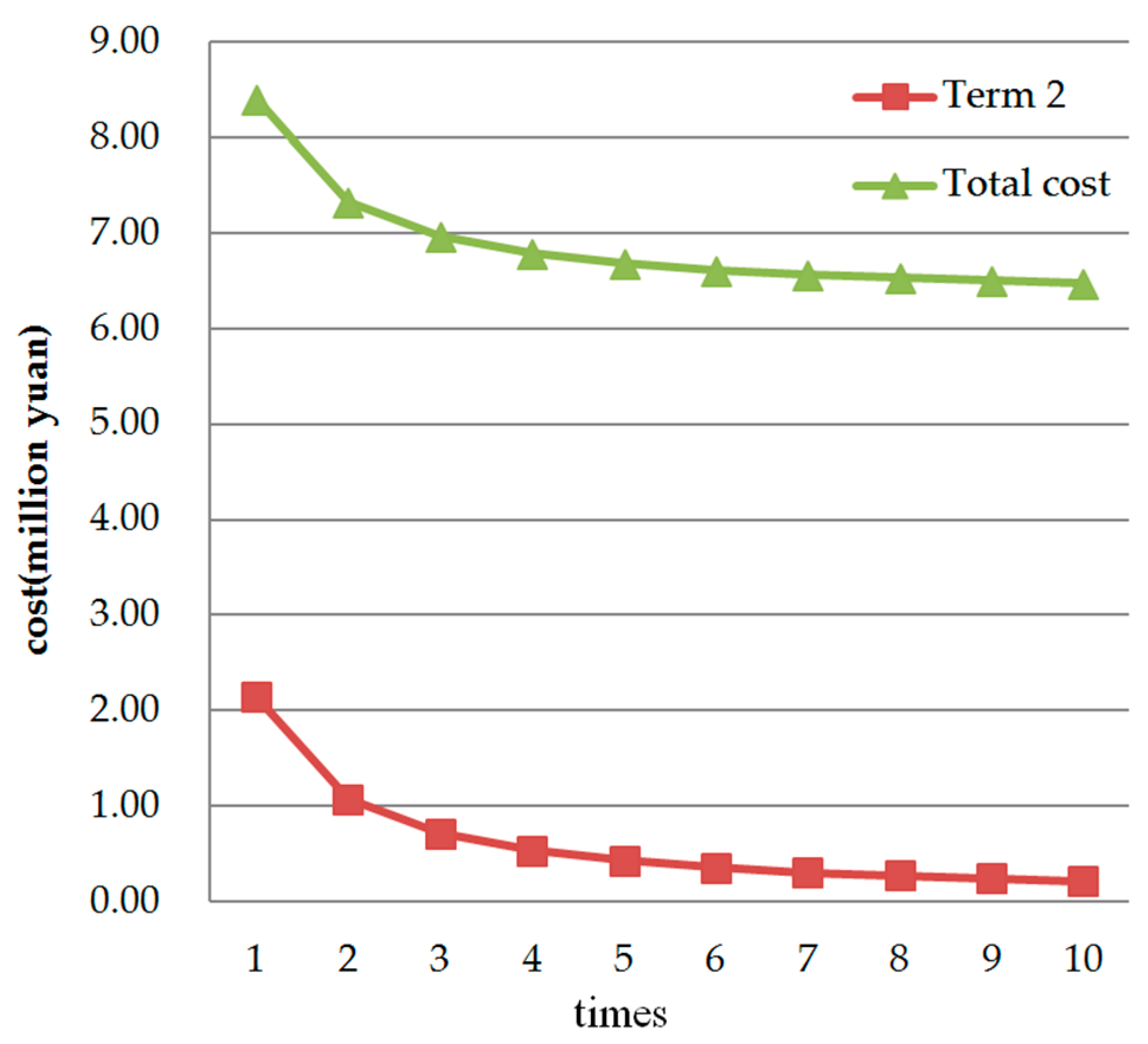
4.2.1. Charging Speed
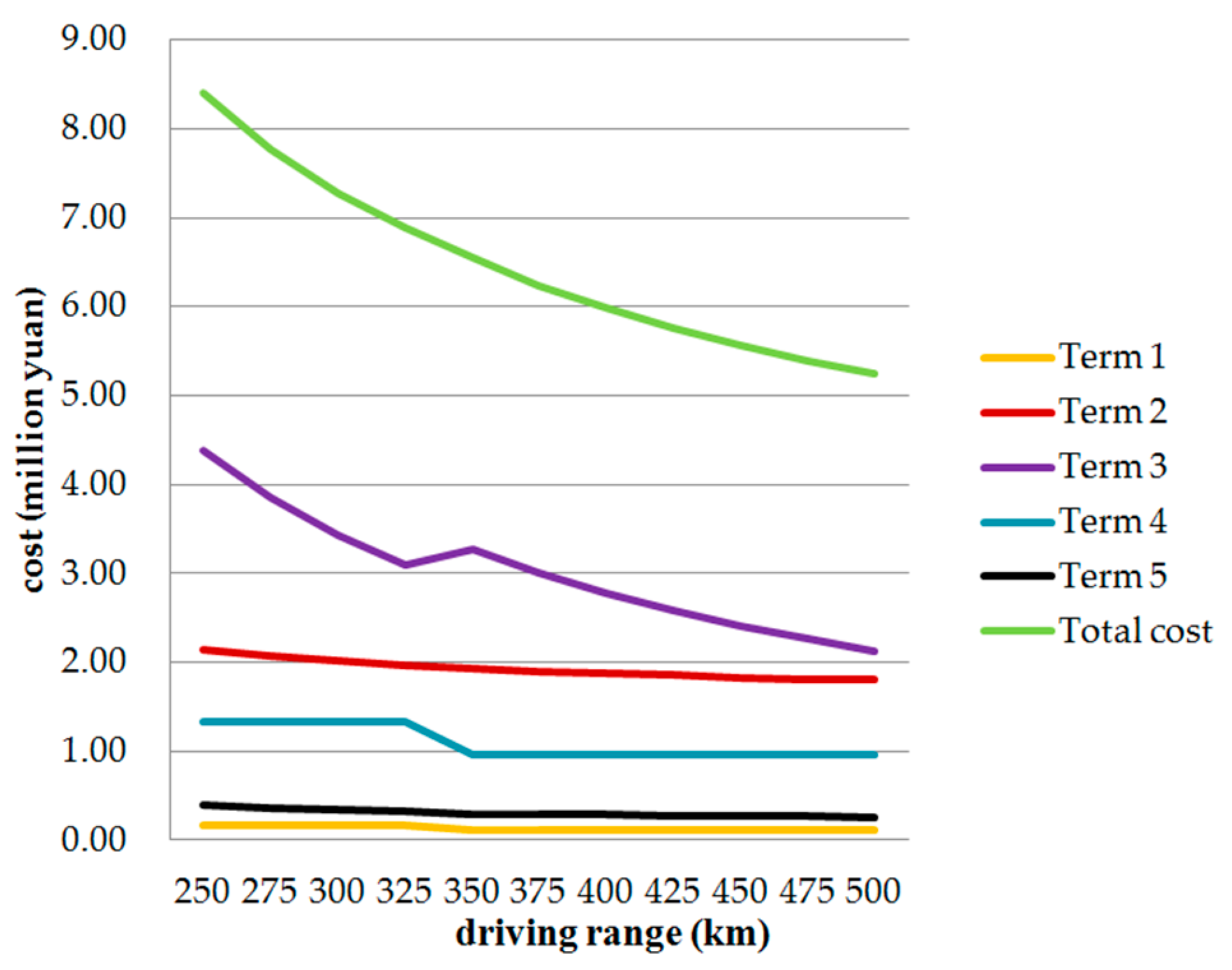
4.2.2. Driving Range
4.2.3. Analyses and Findings
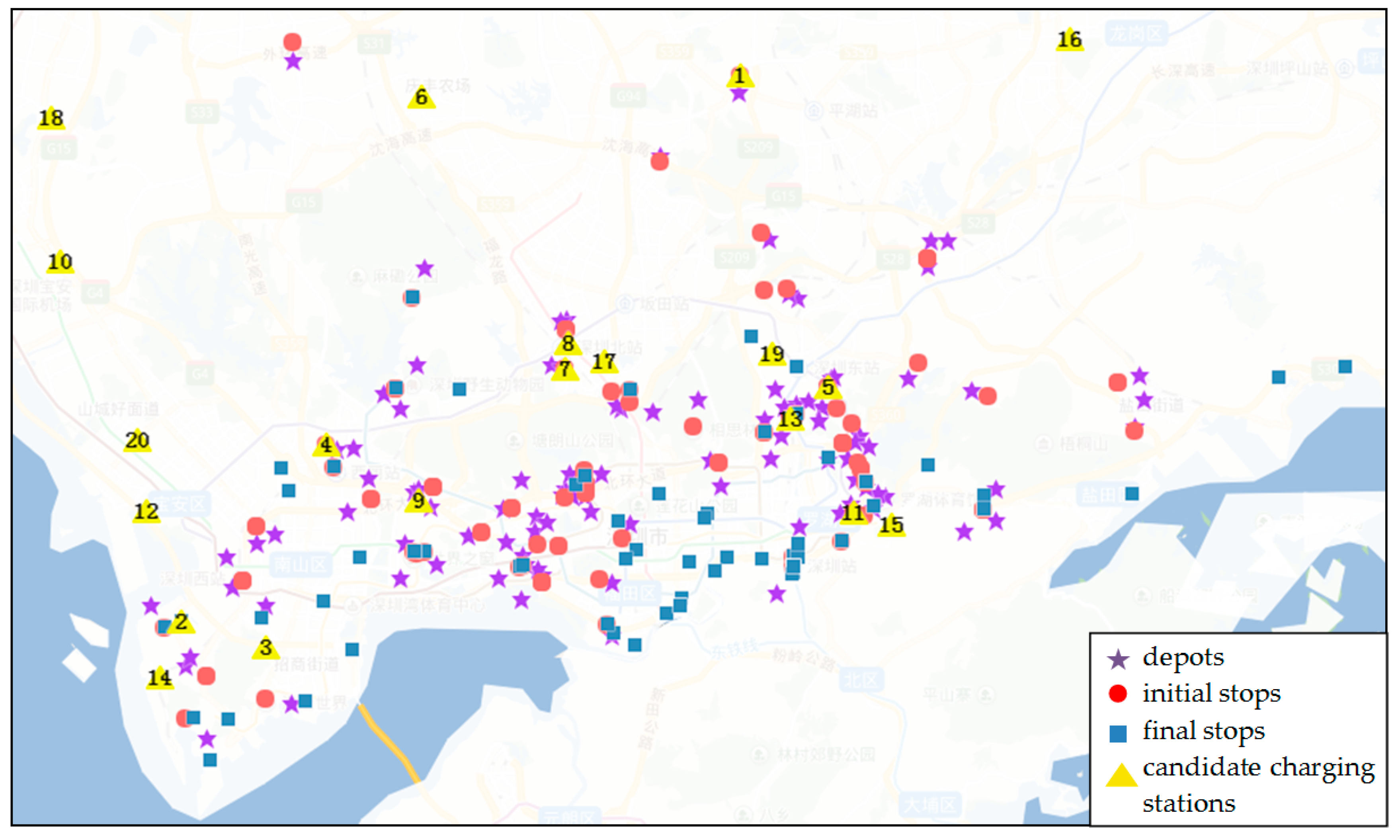
4.3. Real-World Transportation Network in Shenzhen
5. Conclusions and Future Work
Supplementary Materials
Author Contributions
Funding
Acknowledgments
Conflicts of Interest
References
- Ye, B.; Jiang, J.; Miao, L.; Yang, P.; Li, J.; Shen, B. Feasibility Study of a Solar-Powered Electric Vehicle Charging Station Model. Energies 2015, 8, 13265–13283. [Google Scholar] [CrossRef]
- Tang, J.; Ye, B.; Lu, Q.; Wang, D.; Li, J. Economic Analysis of Photovoltaic Electricity Supply for an Electric Vehicle Fleet in Shenzhen, China. Int. J. Sustain. Transp. 2013, 8, 202–224. [Google Scholar] [CrossRef]
- Ministry of Ecology and Environment of China. China Vehicle Environmental Management Annual Report 2018; Ministry of Ecology and Environment of China: Beijing, China, 2018.
- Li, G. The Report of Green Travel Trend. Available online: http://epaper.21jingji.com/html/2018-02/07/content_80354.htm (accessed on 29 July 2019).
- Jiang, J.; Ye, B.; Ma, X.; Miao, L. Controlling GHG emissions from the transportation sector through an ETS: Institutional arrangements in Shenzhen, China. Clim. Policy 2015, 16, 353–371. [Google Scholar] [CrossRef]
- Bak, D.-B.; Bak, J.-S.; Kim, S.-Y. Strategies for Implementing Public Service Electric Bus Lines by Charging Type in Daegu Metropolitan City, South Korea. Sustainability 2018, 10, 3386. [Google Scholar] [CrossRef]
- World Resources Institute. How Did Shenzhen, China Build World’s Largest Electric Bus Fleet? Available online: https://www.wri.org/blog/2018/04/how-did-shenzhen-china-build-world-s-largest-electric-bus-fleet (accessed on 29 June 2019).
- Zart, N. 100% Electric Bus Fleet for Shenzhen (Population 11.9 Million) by End of 2017. Available online: https://cleantechnica.com/2017/11/12/100-electric-bus-fleet-shenzhen-pop-11-9-million-end-2017/ (accessed on 26 May 2019).
- Yu, J.; Yang, P.; Zhang, K.; Wang, F.; Miao, L. Evaluating the Effect of Policies and the Development of Charging Infrastructure on Electric Vehicle Diffusion in China. Sustainability 2018, 10, 3394. [Google Scholar] [CrossRef]
- Wang, F.-P.; Yu, J.-L.; Yang, P.; Miao, L.-X.; Ye, B. Analysis of the Barriers to Widespread Adoption of Electric Vehicles in Shenzhen China. Sustainability 2017, 9, 522. [Google Scholar] [CrossRef]
- National Development and Reform Commission of China. Guidelines for Charging Infrastructure Development of Electric Vehicles (2015–2020); National Development and Reform Commission of China: Beijing, China, 2015.
- Lv, S. 100% Pure Electric Bus Fleet in Shenzhen, the Largest in the World. Available online: https://society.hubpd.com/c/2018-05-08/738624.shtml (accessed on 29 June 2019).
- Shenzhen Evening News. Yueliangwan Intergated Station Will Open Next May. Available online: http://wb.sznews.com/PC/layout/201808/21/node_A03.html#content_444640 (accessed on 29 June 2019).
- Li, W.; Li, Y.; Deng, H.; Bao, L. Planning of Electric Public Transport System under Battery Swap Mode. Sustainability 2018, 10, 2528. [Google Scholar] [CrossRef]
- Huang, M.; Li, J.-Q. The Shortest Path Problems in Battery-Electric Vehicle Dispatching with Battery Renewal. Sustainability 2016, 8, 607. [Google Scholar] [CrossRef]
- Muratori, M. Impact of uncoordinated plug-in electric vehicle charging on residential power demand. Nat. Energy 2018, 3, 193–201. [Google Scholar] [CrossRef]
- Zheng, Y.; Dong, Z.Y.; Xu, Y.; Meng, K.; Zhao, J.H.; Qiu, J. Electric Vehicle Battery Charging/Swap Stations in Distribution Systems: Comparison Study and Optimal Planning. IEEE Trans. Power Syst. 2014, 29, 221–229. [Google Scholar] [CrossRef]
- Helber, S.; Broihan, J.; Jang, Y.; Hecker, P.; Feuerle, T. Location Planning for Dynamic Wireless Charging Systems for Electric Airport Passenger Buses. Energies 2018, 11, 258. [Google Scholar] [CrossRef]
- Sohu Auto. Battery Charging or Swapping? Does the Swapping Mode Have a Future? Available online: http://www.sohu.com/a/118489915_180553 (accessed on 29 July 2019).
- Auto Observer. What is Lifetime Warranty of EV Batteries? Available online: https://chejiahao.autohome.com.cn/info/2757357/ (accessed on 1 July 2019).
- Liu, Z.; Song, Z. Robust planning of dynamic wireless charging infrastructure for battery electric buses. Transp. Res. Part C Emerg. Technol. 2017, 83, 77–103. [Google Scholar] [CrossRef]
- Baijiahao. How Much Does it Cost to Replace an EV Battery? The Reveal of the Battery Replacement Cost for Different Auto Brands. Available online: https://baijiahao.baidu.com/s?id=1605689212409993781&wfr=spider&for=pc (accessed on 3 July 2019).
- Liu, Z.; Song, Z.; He, Y. Optimal Deployment of Dynamic Wireless Charging Facilities for an Electric Bus System. Transp. Res. Rec. J. Transp. Res. Board 2017, 2647, 100–108. [Google Scholar] [CrossRef]
- Netease Auto. Shenzhen Mode Goes Out of Shenzhen: How to Commercialize New-Energy Vehicles? Available online: http://auto.163.com/12/0322/11/7T6QK4MM00084TV1.html (accessed on 5 July 2019).
- Ciez, R.E.; Whitacre, J.F. Examining different recycling processes for lithium-ion batteries. Nat. Sustain. 2019, 2, 148–156. [Google Scholar] [CrossRef]
- Chinabuses. BYD Bus--BYD6121LGEV4. Available online: http://www.chinabuses.com/product/buses/12103.html (accessed on 29 June 2019).
- D1EV. Shenzhen Mode Explores the Market-Oriented Operational Way. Available online: https://www.d1ev.com/news/shichang/22929 (accessed on 7 July 2019).
- Kunith, A.; Mendelevitch, R.; Goehlich, D. Electrification of a city bus network—An optimization model for cost-effective placing of charging infrastructure and battery sizing of fast-charging electric bus systems. Int. J. Sustain. Transp. 2017, 11, 707–720. [Google Scholar] [CrossRef]
- Ko, Y.D.; Jang, Y.J. The Optimal System Design of the Online Electric Vehicle Utilizing Wireless Power Transmission Technology. IEEE Trans. Intell. Transp. Syst. 2013, 14, 1255–1265. [Google Scholar] [CrossRef]
- Jang, Y.J.; Jeong, S.; Ko, Y.D. System optimization of the On-Line Electric Vehicle operating in a closed environment. Comput. Ind. Eng. 2015, 80, 222–235. [Google Scholar] [CrossRef]
- He, Y.; Song, Z.; Liu, Z. Fast-charging station deployment for battery electric bus systems considering electricity demand charges. Sustain. Cities Soc. 2019, 48, 101530. [Google Scholar] [CrossRef]
- Liu, Z.; Song, Z.; He, Y. Economic Analysis of On-Route Fast Charging for Battery Electric Buses: Case Study in Utah. Transp. Res. Rec. J. Transp. Res. Board 2019, 2673, 036119811983997. [Google Scholar] [CrossRef]
- Wang, Y.-W.; Lin, C.-C. Locating road-vehicle refueling stations. Transp. Res. Part E Logist. Transp. Rev. 2009, 45, 821–829. [Google Scholar] [CrossRef]
- Huang, Y.; Li, S.; Qian, Z.S. Optimal Deployment of Alternative Fueling Stations on Transportation Networks Considering Deviation Paths. Netw. Spat. Econ. 2015, 15, 183–204. [Google Scholar] [CrossRef]
- Li, S.; Huang, Y.; Mason, S.J. A multi-period optimization model for the deployment of public electric vehicle charging stations on network. Transp. Res. Part C Emerg. Technol. 2016, 65, 128–143. [Google Scholar] [CrossRef]
- Xylia, M.; Leduc, S.; Patrizio, P.; Kraxner, F.; Silveira, S. Locating charging infrastructure for electric buses in Stockholm. Transp. Res. Part C Emerg. Technol. 2017, 78, 183–200. [Google Scholar] [CrossRef]
- Liu, Z.; Song, Z.; He, Y. Planning of Fast-Charging Stations for a Battery Electric Bus System under Energy Consumption Uncertainty. Transp. Res. Rec. J. Transp. Res. Board 2018, 2672, 036119811877295. [Google Scholar] [CrossRef]
- Bi, Z.; Keoleian, G.A.; Ersal, T. Wireless charger deployment for an electric bus network: A multi-objective life cycle optimization. Appl. Energy 2018, 225, 1090–1101. [Google Scholar] [CrossRef]
- Yilmaz, M.; Krein, P.T. Review of Battery Charger Topologies, Charging Power Levels, and Infrastructure for Plug-In Electric and Hybrid Vehicles. IEEE Trans. Power Electron. 2013, 28, 2151–2169. [Google Scholar] [CrossRef]
- Liu, H.; Wang, D.Z.W. Locating multiple types of charging facilities for battery electric vehicles. Transp. Res. Part B Methodol. 2017, 103, 30–55. [Google Scholar] [CrossRef]
- Tencent Auto. The Introduction of Pure Electric Bus BYD K9. Available online: https://auto.qq.com/a/20100930/000164.htm (accessed on 9 July 2019).
- Rogge, M.; Wollny, S.; Sauer, D. Fast Charging Battery Buses for the Electrification of Urban Public Transport—A Feasibility Study Focusing on Charging Infrastructure and Energy Storage Requirements. Energies 2015, 8, 4587–4606. [Google Scholar] [CrossRef]
- Rogge, M.; van der Hurk, E.; Larsen, A.; Sauer, D.U. Electric bus fleet size and mix problem with optimization of charging infrastructure. Appl. Energy 2018, 211, 282–295. [Google Scholar] [CrossRef]
- Ke, B.-R.; Chung, C.-Y.; Chen, Y.-C. Minimizing the costs of constructing an all plug-in electric bus transportation system: A case study in Penghu. Appl. Energy 2016, 177, 649–660. [Google Scholar] [CrossRef]
- Chen, Z.; Yin, Y.; Song, Z. A cost-competitiveness analysis of charging infrastructure for electric bus operations. Transp. Res. Part C Emerg. Technol. 2018, 93, 351–366. [Google Scholar] [CrossRef]
- Jang, Y.; Jeong, S.; Lee, M. Initial Energy Logistics Cost Analysis for Stationary, Quasi-Dynamic, and Dynamic Wireless Charging Public Transportation Systems. Energies 2016, 9, 483. [Google Scholar] [CrossRef]
- Bi, Z.; Song, L.; De Kleine, R.; Mi, C.C.; Keoleian, G.A. Plug-in vs. wireless charging: Life cycle energy and greenhouse gas emissions for an electric bus system. Appl. Energy 2015, 146, 11–19. [Google Scholar] [CrossRef]
- Paul, T.; Yamada, H. Operation and charging scheduling of electric buses in a city bus route network. In Proceedings of the 2014 IEEE 17th International Conference on Intelligent Transportation Systems (ITSC), Qingdao, China, 8–11 October 2014; pp. 2780–2786. [Google Scholar]
- Ding, H.; Hu, Z.; Song, Y. Value of the energy storage system in an electric bus fast charging station. Appl. Energy 2015, 157, 630–639. [Google Scholar] [CrossRef]
- Hu, X.; Murgovski, N.; Johannesson, L.; Egardt, B. Energy efficiency analysis of a series plug-in hybrid electric bus with different energy management strategies and battery sizes. Appl. Energy 2013, 111, 1001–1009. [Google Scholar] [CrossRef]
- Chen, H.; Hu, Z.; Zhang, H.; Luo, H. Coordinated charging and discharging strategies for plug-in electric bus fast charging station with energy storage system. IET Gener. Transm. Distrib. 2018, 12, 2019–2028. [Google Scholar] [CrossRef]
- Li, L.; Yang, C.; Zhang, Y.; Zhang, L.; Song, J. Correctional DP-based energy management strategy of plug-in hybrid electric bus for city-bus route. IEEE Trans. Veh. Technol. 2015, 64, 2792–2803. [Google Scholar] [CrossRef]
- Galiveeti, H.R.; Goswami, A.K.; Dev Choudhury, N.B. Impact of plug-in electric vehicles and distributed generation on reliability of distribution systems. Eng. Sci. Technol. Int. J. 2018, 21, 50–59. [Google Scholar] [CrossRef]
- Green, R.C.; Wang, L.; Alam, M. The impact of plug-in hybrid electric vehicles on distribution networks: A review and outlook. Renew. Sustain. Energy Rev. 2011, 15, 544–553. [Google Scholar] [CrossRef]
- He, F.; Wu, D.; Yin, Y.; Guan, Y. Optimal deployment of public charging stations for plug-in hybrid electric vehicles. Transp. Res. Part B Methodol. 2013, 47, 87–101. [Google Scholar] [CrossRef]
- Wang, G.; Xu, Z.; Wen, F.; Wong, K.P. Traffic-constrained multiobjective planning of electric-vehicle charging stations. IEEE Trans. Power Deliv. 2013, 28, 2363–2372. [Google Scholar] [CrossRef]
- Apostolaki-Iosifidou, E.; Codani, P.; Kempton, W. Measurement of power loss during electric vehicle charging and discharging. Energy 2017, 127, 730–742. [Google Scholar] [CrossRef]
- Mak, H.-Y.; Rong, Y.; Shen, Z.-J.M. Infrastructure Planning for Electric Vehicles with Battery Swapping. Manag. Sci. 2013, 59, 1557–1575. [Google Scholar] [CrossRef]
- Sortomme, E.; Hindi, M.M.; MacPherson, S.J.; Venkata, S. Coordinated charging of plug-in hybrid electric vehicles to minimize distribution system losses. IEEE Trans. Smart Grid 2011, 2, 198–205. [Google Scholar] [CrossRef]
- Cao, C.; Wang, L.; Chen, B. Mitigation of the Impact of High Plug-in Electric Vehicle Penetration on Residential Distribution Grid Using Smart Charging Strategies. Energies 2016, 9, 1024. [Google Scholar] [CrossRef]
- Wang, L.; Chen, B. Distributed control for large-scale plug-in electric vehicle charging with a consensus algorithm. Int. J. Electr. Power Energy Syst. 2019, 109, 369–383. [Google Scholar] [CrossRef]
- Zhang, H.; Moura, S.; Hu, Z.; Song, Y. PEV Fast-Charging Station Siting and Sizing on Coupled Transportation and Power Networks. IEEE Trans. Smart Grid 2016, 9, 2595–2605. [Google Scholar] [CrossRef]
- Wei, W.; Mei, S.; Wu, L.; Shahidehpour, M.; Fang, Y. Optimal Traffic-Power Flow in Urban Electrified Transportation Networks. IEEE Trans. Smart Grid 2017, 8, 84–95. [Google Scholar] [CrossRef]
- Shenzhen Economic Daily. The Scale of New-Energy Buses in Shenzhen, Guangdong is Number One in the World. Available online: http://www.chinarta.com/html/2014-6/201469132646.htm (accessed on 16 July 2019).
- Development and Reform Commission of Guangdong Province. The planning of electric vehicle charging infrastructure in Guangdong Province (2016–2020). Available online: http://www.cecol.com.cn/news/20171108/11423708.html (accessed on 12 July 2019).
- Farivar, M.; Low, S.H. Branch Flow Model: Relaxations and Convexification—Part I. IEEE Trans. Power Syst. 2013, 28, 2554–2564. [Google Scholar] [CrossRef]
- Gan, L.; Li, N.; Topcu, U.; Low, S.H. Exact Convex Relaxation of Optimal Power Flow in Radial Networks. IEEE Trans. Autom. Control 2015, 60, 72–87. [Google Scholar] [CrossRef]
- Atamtürk, A.; Berenguer, G.; Shen, Z.-J. A Conic Integer Programming Approach to Stochastic Joint Location-Inventory Problems. Oper. Res. 2012, 60, 366–381. [Google Scholar] [CrossRef]
- BYD. K9 introduction. Available online: http://www.bydauto.com.cn/car-show-K9.html (accessed on 29 June 2019).


| Sets | |
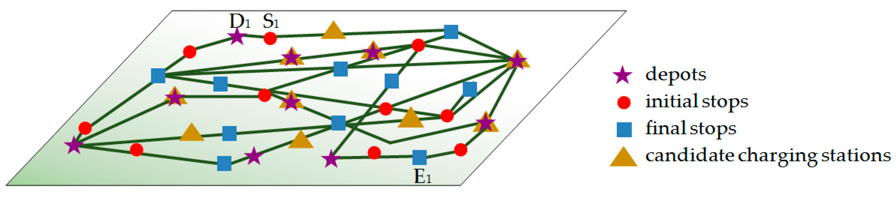
| set of bus lines | |
| set of origins of bus charging trips, including bus depots, final stops, and initial stops | |
| set of candidates charging station locations, which could be the bus depots that can be reconstructed to add charging station function or other new locations | |
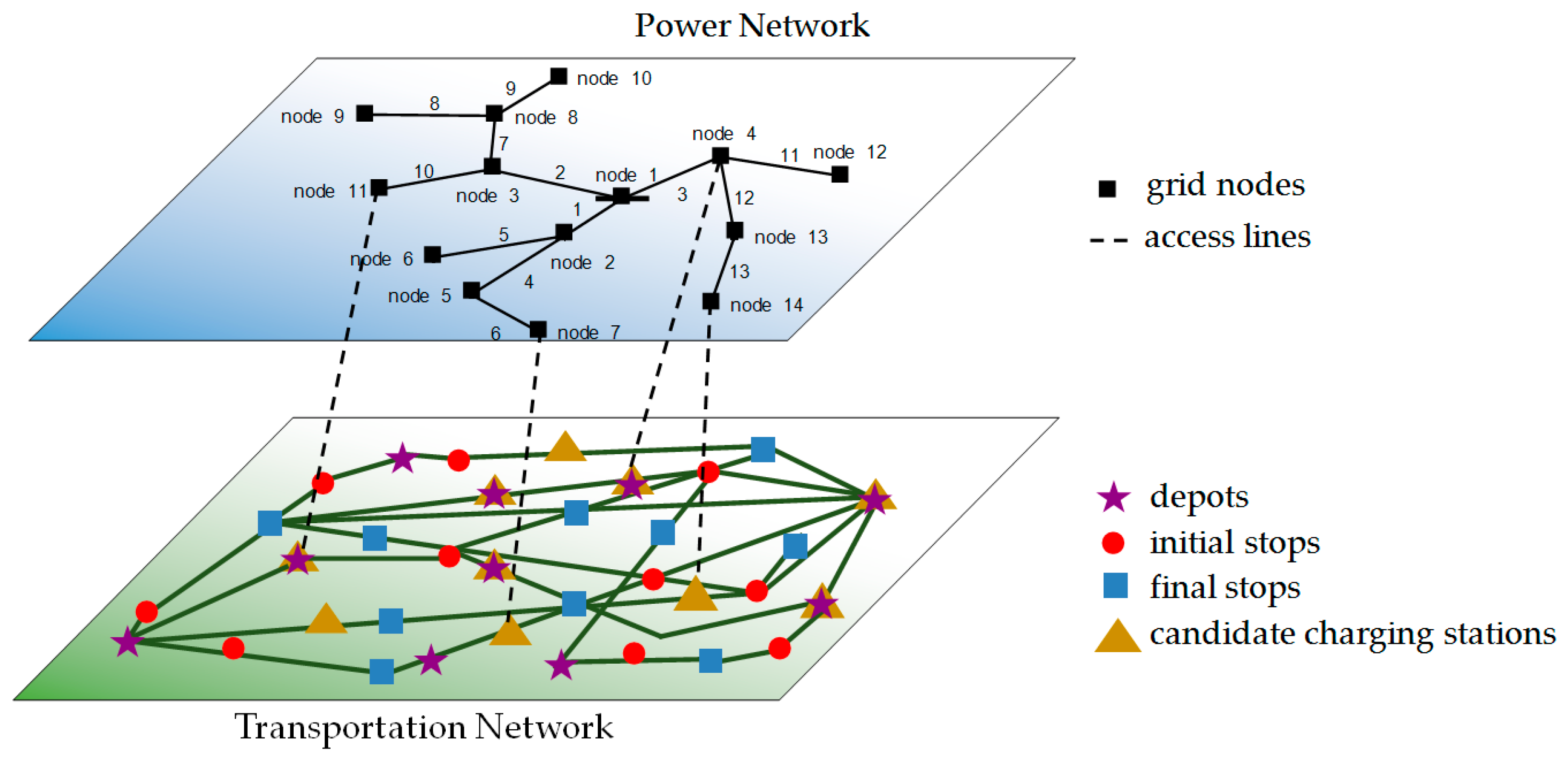
| set of power grid nodes | |
| Parameters | |
| the number of e-buses of bus line | |
| charging time required for a full battery charge | |
| battery capacity of e-buses | |
| charger working time per day | |
| charging frequency. E-buses go for charging every day(s) | |
| the number of charging trips of buses in bus line per year | |
| the demand for chargers of bus line | |
| annual fixed costs of location , which could be the construction cost of a new station that includes the price of land, or the reconstruction cost of original bus depots | |
| annual unit cost of chargers | |
| driving range of an electric bus | |
| distance from of bus line to location | |
| transportation cost per kilometer, which is measured by the product of electricity consumed per kilometer and the market price of electricity | |
| annual line construction cost to connect location to power grid node . | |
| charging speed/the power of charger | |
| original loads of node | |
| the maximal loads of the power grid | |
| denotes the impedance of branch where and denote the resistance and reactance, respectively | |
| annual power loss time of branch | |
| unit price of electricity | |
| the original square of the magnitude of the complex current from node to node before charging stations connect to the power grid | |
| voltage limit of node , is the square of the magnitude of the complex voltage | |
| current limit of branch , is the square of the magnitude of the complex current | |
| Decision variables | |
| if the charging station is built at location otherwise | |
| , if buses of bus line start from to a charging station; , otherwise. | |
| if buses of bus line are assigned to location for charging; , otherwise | |
| if location is assigned to power grid node otherwise. | |
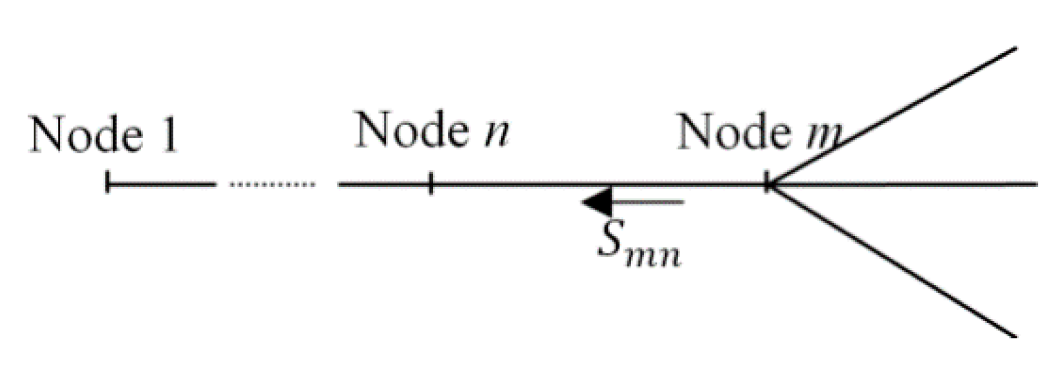
| denotes the sending-end power flow from node to node , where and denote the real and reactive power flow, respectively | |
| denotes the power injection of node where and denote the real and reactive power injection, respectively | |
| the square of the voltage magnitude of node | |
| the square of the current magnitude of branch | |
| [LN, SN, GN] | Computational Time (Seconds) | ||
|---|---|---|---|
| No R | |||
| [15, 5, 10] | 5.9 | 4.5 | 2.1 |
| [20, 7, 12] | 34.1 | 6.3 | 2.3 |
| [25, 8, 14] | 439.5 | 8.5 | 3.0 |
| [27, 8, 14] | 3234.9 | 9.3 | 3.2 |
| [30, 10, 14] | 14,188.6 | 12.2 | 3.3 |
| [35, 12, 14] | >20 h | 25.7 | 3.9 |
| [40, 13, 14] | >20 h | 41.8 | 4.4 |
| [70, 17, 14] | >20 h | 95.1 | 11.2 |
| [80, 17, 14] | >20 h | 100.3 | 16.0 |
| [81, 17, 14] | >20 h | 242.2 | 16.1 |
| [81, 18, 14] | >20 h | 308.6 | 16.4 |
| [90, 18, 14] | >20 h | >20 h | 20.7 |
| [100, 20, 14] | >20 h | >20 h | 90.2 |
| Line | Origin | CS | Line | Origin | CS |
|---|---|---|---|---|---|
| 1 | 2 | 11 | 11 | 3 | 11 |
| 2 | 2 | 13 | 12 | 2 | 11 |
| 3 | 1 | 11 | 13 | 2 | 11 |
| 4 | 1 | 11 | 14 | 1 | 11 |
| 5 | 3 | 11 | 15 | 1 | 13 |
| 6 | 3 | 11 | 16 | 1 | 9 |
| 7 | 3 | 11 | 17 | 3 | 9 |
| 8 | 3 | 11 | 18 | 3 | 9 |
| 9 | 3 | 11 | 19 | 2 | 11 |
| 10 | 3 | 11 | 20 | 1 | 9 |
| Times | Charging Power (Kw) | Cost (Million Yuan) | Layout | ||
|---|---|---|---|---|---|
| Term 2 | Total Cost | Stations Selected | Grid Nodes Connected | ||
| 1 | 108 | 2.15 | 8.41 | 9, 11, 13 | 2, 2, 14 |
| 2 | 216 | 1.07 | 7.33 | 9, 11, 13 | 2, 2, 14 |
| 3 | 324 | 0.72 | 6.98 | 9, 11, 13 | 2, 2, 14 |
| 4 | 432 | 0.54 | 6.80 | 9, 11, 13 | 2, 2, 14 |
| 5 | 540 | 0.43 | 6.69 | 9, 11, 13 | 2, 2, 14 |
| 6 | 648 | 0.36 | 6.62 | 9, 11, 13 | 2, 2, 14 |
| 7 | 756 | 0.31 | 6.57 | 9, 11, 13 | 2, 2, 14 |
| 8 | 864 | 0.27 | 6.53 | 9, 11, 13 | 2, 2, 14 |
| 9 | 972 | 0.24 | 6.50 | 9, 11, 13 | 2, 2, 14 |
| 10 | 1080 | 0.21 | 6.48 | 9, 11, 13 | 2, 2, 14 |
| Driving Range (Km) | Cost (Million Yuan) | Layout | ||||||
|---|---|---|---|---|---|---|---|---|
| Term 1 | Term 2 | Term 3 | Term 4 | Term 5 | Total Cost | Stations Selected | Grid Nodes Connected | |
| 250 | 0.16 | 2.15 | 4.38 | 1.33 | 0.39 | 8.41 | 9, 11, 13 | 2, 2, 14 |
| 275 | 0.16 | 2.07 | 3.85 | 1.33 | 0.36 | 7.77 | 9, 11, 13 | 2, 2, 14 |
| 300 | 0.16 | 2.01 | 3.43 | 1.33 | 0.34 | 7.28 | 9, 11, 13 | 2, 2, 14 |
| 325 | 0.16 | 1.97 | 3.10 | 1.33 | 0.33 | 6.88 | 9, 11, 13 | 2, 2, 14 |
| 350 | 0.11 | 1.93 | 3.27 | 0.95 | 0.29 | 6.55 | 9, 11 | 2, 2 |
| 375 | 0.11 | 1.90 | 3.00 | 0.95 | 0.29 | 6.24 | 9, 11 | 2, 2 |
| 400 | 0.11 | 1.87 | 2.77 | 0.95 | 0.28 | 5.98 | 9, 11 | 2, 2 |
| 425 | 0.11 | 1.85 | 2.58 | 0.95 | 0.27 | 5.75 | 9, 11 | 2, 2 |
| 450 | 0.11 | 1.83 | 2.41 | 0.95 | 0.27 | 5.56 | 9, 11 | 2, 2 |
| 475 | 0.11 | 1.81 | 2.26 | 0.95 | 0.26 | 5.39 | 9, 11 | 2, 2 |
| 500 | 0.11 | 1.80 | 2.13 | 0.95 | 0.26 | 5.24 | 9, 11 | 2, 2 |
| Stations Selected | Number of Chargers Installed | Grid Nodes Connected |
|---|---|---|
| 2 | 124 | 4 |
| 4 | 80 | 13 |
| 8 | 93 | 4 |
| 11 | 191 | 2 |
| 12 | 41 | 6 |
| 19 | 111 | 2 |
| 24 | 138 | 3 |
| 25 | 63 | 3 |
| 27 | 86 | 3 |
| 29 | 120 | 12 |
| 30 | 99 | 5 |
© 2019 by the authors. Licensee MDPI, Basel, Switzerland. This article is an open access article distributed under the terms and conditions of the Creative Commons Attribution (CC BY) license (http://creativecommons.org/licenses/by/4.0/).
Share and Cite
Lin, Y.; Zhang, K.; Shen, Z.-J.M.; Miao, L. Charging Network Planning for Electric Bus Cities: A Case Study of Shenzhen, China. Sustainability 2019, 11, 4713. https://doi.org/10.3390/su11174713
Lin Y, Zhang K, Shen Z-JM, Miao L. Charging Network Planning for Electric Bus Cities: A Case Study of Shenzhen, China. Sustainability. 2019; 11(17):4713. https://doi.org/10.3390/su11174713
Chicago/Turabian StyleLin, Yuping, Kai Zhang, Zuo-Jun Max Shen, and Lixin Miao. 2019. "Charging Network Planning for Electric Bus Cities: A Case Study of Shenzhen, China" Sustainability 11, no. 17: 4713. https://doi.org/10.3390/su11174713
APA StyleLin, Y., Zhang, K., Shen, Z.-J. M., & Miao, L. (2019). Charging Network Planning for Electric Bus Cities: A Case Study of Shenzhen, China. Sustainability, 11(17), 4713. https://doi.org/10.3390/su11174713