Abstract
Accurate forecasting of the hotel accommodation demands is extremely critical to the sustainable development of tourism-related industries. In view of the ever-increasing tourism data, this paper constructs a deep learning framework to handle the prediction problem in the hotel accommodation demands. Taking China’s Hainan province as an empirical example, the internet search index is used from August 2008 to May 2019 to forecast the overnight passenger flows for hotels accommodation in Hainan Province, China. Forecasting results indicate that compared to benchmark models, the constructed forecasting method can effectively simulate dynamic characteristics of the overnight passenger flows for the hotel accommodation and significantly improve the forecasting performance of the model. Forecasting results can provide necessary references for decision-making in tourism-related industries, and this forecasting framework can also be extended to other similar complex time series forecasting problems.
1. Introduction
The tourist hotel is an important part of the tourism industry. The tourist destination hotels flow is the indicator of hotel revenue; accurate passenger flow forecasting is the key link in the hotel revenue management [1], which helps related companies and organizations allocate limited tourism resources scientifically and reasonably to maintain market competitiveness [2]. However, the tourism demands such as the overnight passenger flow of hotels has characteristics of complex nonlinear fluctuations. The uncertainty of the passenger flow during the tourist season makes the decision-making of relevant departments into a dilemma, either overestimating or underestimating of the passenger flow will result in unnecessary waste of resources in tourism-related industries; additionally, the actual overnight passenger flow released by the statistical department has serious hysteresis. On the other hand, existing non-linear prediction methods are difficult to adapt to the increasing experimental data, and unable to extract feature information automatically, affecting the forecasting accuracy. With the all-round development of the Internet, a large amount of online query index generated by the consumer information search provides a new direction for an overnight traffic forecasting of tourist hotels [3]. This study addresses the aforementioned problems and expands the previous research by introducing appropriate nonlinear forecasting methods and constructing deep learning (DL) forecasting frameworks.
Existing prediction methods of tourism demands include linear and nonlinear technologies. Linear forecasting technologies mainly include the time series forecasting models represented by the autoregressive integrated moving average (ARIMA) and econometric models. Nevertheless, these methods need to meet the stability of the economic environment and the stability assumptions of the time series. In practice, it is often unable to fully simulate complex nonlinear characteristics of the destination demands [4]. The nonlinear technologies represented by the regression version of the support vector machine (SVR) method have certain nonlinear forecasting abilities when dealing with small sample data sets [4,5,6], but these methods are shallow learning technologies. Hence, in the aspect of practical applications, it’s hard for these methods to meet the growing data samples. Additionally, these methods cannot automatically extract features information, but also easily fall into the local optimum as well as over-fitting problems.
With the comprehensive development of the Internet, the information query has become a crucial basis for decision-making [7,8]. A large number of records generated by information query possess real-time and accessible features. These data mainly from the Baidu or Google search engine are objective reflections of consumers’ latent demands for travel and have become increasingly important for tourism demand forecasting [3].
Existing literatures mainly use the consumer search data to forecast the tourist flow in scenic areas. Predictive results based on the linear model suggested that the Internet search index can improve the forecasting performance [9,10,11,12,13]. For instance, Yang et al. [11] applied the web index from Google and Baidu as input sets of the ARIMA model for a comparative study on the Chinese tourist volume. Huang et al. [12] used the query data from Baidu as a predictive variable of the ARIMA model to forecast the tourist arrivals of the Imperial Palace in Beijing. Taking Xi’an as an example, Wei and Cui [13] used the seasonal adjustment method to explore the correlation between the search data from Baidu and the tourist flow. However, the linear model needs to satisfy the stationary assumption of the time series and the stable economic environment, and it is difficult to effectively simulate the nonlinear relationship of tourism demands.
In order to cope with the nonlinear, existing literature used the Internet query index as input sets of nonlinear tools such as the artificial neural network (ANN) and the regression version of the support vector machine, to predict the tourist flow [5,6,14]. For example, Sun et al. [6] applied the web query data to construct a single-layer feed-forward neural network (FFNN) to simulate the tourist flows in Beijing. The empirical analysis shows that the search query data can effectively fit the dynamic characteristics of the tourist arrivals and improve the predictive accuracy of the constructed method. Li et al. [14] developed a composite forecasting tool using the back propagation algorithm (BPNN) and used the Baidu index to predict the tourist volume. Despite this, models such as the SVR and ANN are essentially shallow learning methods that are difficult to meet the growing samples of the tourism data, and challenge the predictive accuracy.
Previous studies forecasted the demands of tourist hotels mainly based on linear models [15,16,17,18,19]. For example, Choi [18] identified key economic indicators of the hotel industry in the US and built synthetic indicators to forecast the US hotel demands successfully. Aliyev et al. [19] used fuzzy time series models to forecast the hotel occupancy. There was very rare research specializing in the hotel demand forecasting using the Internet search data. For example, Pan et al. [20] utilize the Google trend index as model inputs to forecast the hotel occupancy. The results indicated that the addition of network queries can obviously reduce the prediction error. However, these studies mainly use the Google trend data as predictive variables of linear models. In China, consumers mainly use the Baidu search engine for information search. There is no relevant literature using the Baidu search data to forecast the demands for the tourist hotel accommodation. Whether the Baidu search data has a predictive effect on the demands of tourist hotels remains to be investigated. In addition, with the increase in the data samples, linear-based forecasting techniques are difficult to fully simulate the nonlinearity of the hotel accommodation demands.
In recent years, with the popularity of artificial intelligence, neural network models with more hidden layers can learn the characteristic information and the relevance behind the complex dataset. The DL technology has attached increasing importance in both academia and the industry [21]. According to the consensus of most current researches, for traditional machine learning algorithms, as the data sample increases, the forecast performance increases according to the power law, but tends to be stable after a while. But for the DL method, its performance increases logarithmically with the increased sample capacity [22]. Compared to other DL models, the long short-term memory (LSTM) exhibits unique advantages in terms of forecasting with sequence as inputs [23,24,25]. In the field of tourism, for example, Chang and Tsai [26] used the deep neural network (DNN) model based on official statistics to forecast Taiwan’s tourist flow. There is no research on the hotel accommodation demand forecasting based upon such DL methods.
The application of the DL models in the complex time series forecasting of tourism demands is explored in this paper. Taking Hainan as an example, the internet search data generated by the consumers’ information search and LSTM models with excellent forecasting ability for the complex time series are used to forecast the overnight passenger flows of tourist hotels. For the purpose of comparing the forecasting power of the developed models, the deep belief network (DBN), BPNN, and C-LSTM (only using past observations of the overnight passenger flow as predictive variables) were constructed as benchmark counterparts. With the empirical results suggesting that the developed LSTM network can effectively forecast hotel demands compared to its competitors.
The contribution of this study to the existing research is twofold. Firstly, we construct a theoretical analysis framework based on the tourism motivation theory and information search behaviour theory for the first time, which provides a theoretical basis for the tourism demand forecasting research based on the web search data. Secondly, unlike previous studies, forecasting tools such as the ANN and SVR cannot adapt to the ever-increasing tourism data. This paper introduces the LSTM with an excellent prediction ability for the complex time series data and constructs an empirical analysis framework to forecast hotel accommodation demands. This method provides a feasible solution for other complex time series predictions under relatively large sample conditions.
2. Theoretical Analysis
It is observed from the tourism motivation theory [27,28] and tourist information search behavior theory [7,29] that tourism is a dynamic process in the temporal and spatial dimension, which can be divided into three stages namely, the pre-tour plan, in-tour experience and post-tour evaluation. The logic framework of the tourist information search is shown in Figure 1.
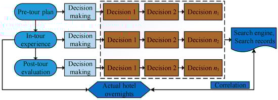
Figure 1.
The logic framework of the tourist information search.
The decision-making of tourism at each stage in the Internet environment relies heavily on the Internet information search. Once a tourism decision is made, tourists will try to fulfill their specific tourism demands. The pre-tour plan refers to a series of plans made by the consumers inspired by the tourism demands. They make tourism decisions by using the Internet to search information thereby, developing an optimal travel plan. The in-tour experience refers to the entire tourism implementation process from the source to the tour destination. It is the process of the tourists’ actual experience on tourism products and services. At this stage, tourists mainly use mobile communication devices such as mobile phones and tablet phones to inquire the tourism-related information they care about, thereby making travel decisions. Post-tour evaluation is an objective evaluation of witnessed tourism products or services after the end of the tour, visitors often use various social media tools to comment on tourism products and services and share their travel experiences.
Jeng and Fesenmaier [30] noted that in the whole process of the pre-tour plan and in-tour experience, tourists would make different tourism decisions for six elements of tourism such as eating, accommodation, transportation, travelling, shopping and entertainment. During this process, the tourists’ potential tourism demands are expressed by the Internet information search on the search engine, which makes a true record of the search information. The consumer information search objectively reflects the tourists’ potential travel motivation. The characteristic information that has the potential influence on the tourism demands can be determined from the Internet information search. The information is the pre-reflection of the passenger flow of tourists destination hotels hence, it becomes an important data source in tourism demand forecasting [3].
3. Design of Forecasting Method
3.1. LSTM Network
The advantage of the traditional recurrent neural network (RNN) model is that it can learn complex temporal dynamic characteristics through the following recurrent equations when dealing with forecasting tasks of sequence input objects:
where, represents the inputs of the model, denotes a hidden layer with the N hidden units, denotes the output at the moment t, and represent the weight and offsets parameters that need to be learned. For the input sequence with the length T, the update of the data is handled in a cycle way.
Although RNN has been successfully applied in areas such as speech recognition as well as text generation [31,32], this method has some difficulties in learning and storing long-term memory information, which can be attributed to disappearing and the explosion of gradients when RNN is optimized in some time steps. The consequence is that the model cannot retain the past memory information over a long time.
LSTM is a variant of RNN, proposed by Hochreiter and Schmidhuber [23] whose core contribution is the introduction of the ingenious concept of self-looping. LSTM provides a solution for a fusion memory cell unit that allows the network to learn the previously forgotten hidden unit and update the hidden unit based on the new information. In addition to the hidden unit , the LSTM network also includes the input gate, forgotten and input adjustment ones, and memory cell. The memory cell unit fuses the state of the previous memory cells, these memory cell units are adjusted by the forgotten gate and the input adjustment gate as well as the previous hidden state, which is adjusted by the input gate. These additional memory cell units enable the LSTM architecture to learn extremely complex long-term time dynamics, ensuring the long-term memory function of the LSTM. The architecture of an LSTM model can be expressed as follows:
where, tanh represents the activation function.
The biggest contribution from RNN is the increased hidden state in LSTM, which determines how much information to add or remove from the previous memory state by using the sigmoid activation function and the point multiplication defined layer. The first gate is the forgotten gate , which controls how much data is discarded from the previous memory state. This is followed by the input gate, which remembers some of the current information and determines which values will be updated. Then, new cell state merges the past and present memory information and selects the information of vector through the forgotten gate, which provides a mechanism for deleting past irrelevant information and adding relevant information from the current time step. Finally, the output layer controls how much memory data will be utilized in the update of the next phase [33].
3.2. Training Method and Model Selection
The back propagation through time (BPTT) commonly used in the RNN network was adopted to train the LSTM network, which is the standard algorithm for training RNN-like network models. The RMSProp, an improved stochastic gradient descent algorithm, was selected for parameter iterative updating. In the LSTM network, in addition to the default activation functions of the model, the other layers use the tanh function as the activation function, which has a more stable gradient and is commonly used in the regression problem.
Over-fitting is an unavoidable phenomenon in the field of DL. The Dropout algorithm developed by Hinton et al. [34] was utilized for solving this defect. This method is a model selection algorithm and a powerful tool to solve the over-fitting in the current DL field.
3.3. Forecasting Framework Construction
After the introduction of the LSTM model, a prediction framework based upon consumer queries was constructed (as shown in Figure 2). This framework illustrates the entire empirical analysis, including keyword selection, variable observations acquisition and cleaning, keyword variable screening, predictive variable selection, experimental dataset construction, forecasting experiment and predictive accuracy test. The detailed steps are as follows:
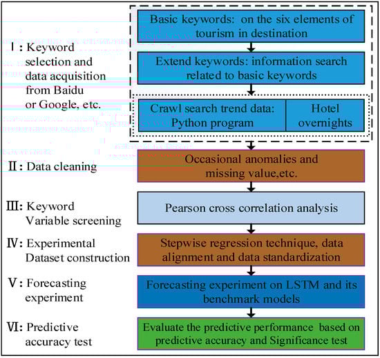
Figure 2.
Logic diagram of the forecasting framework.
Step 1: Experimental dataset acquisition. After determining the search engine, for the purpose of handling the information omission, we selected six elements related to the destination as the benchmark queries, and then inquired extended keywords related to the benchmark keywords circularly. Eventually, we used Python to crawl the structured query volume data of each keyword, and obtained an alternate experimental dataset composed of data of the overnight passenger flow of tourist hotels.
Step 2: Data cleaning. The passenger flow is very sensitive to promotion schemes, emergencies, etc., thereby data may have abnormal values in different periods. In addition, some keyword variables or predicted variables have the problem of missing data, which will affect the prediction of the model. Thus, the individual outliers were replaced by the moving average method, which eliminated the influence of the noise while retaining the basic data characteristics.
Step 3: Predictive variable screening. In order to further find predictive variables that are significantly correlated with the predicted variables, the cross-correlation analysis was used to analyze the connection between the keyword variables and lag variables of the predicted variables. The Pearson cross-correlation analysis is a statistical analysis method, which acquired the Pearson correlation coefficient between the 1–12 order lag variables of the predictive variable and the predicted variable, respectively. The lag variable corresponding to the maximum correlation coefficient was taken as an alternate predictive variable. The threshold was defined, and the keyword variable with the correlation coefficient exceeding was retained as the keyword predictive variable. The same method was used to find the lag variable of the predicted variable as the predictive variable.
Step 4: Experimental dataset construction. For the purpose of reducing the complexity of model training, the stepwise regression analysis was further performed on the potential predictive variables to obtain the final predictive variable with excellent predictive ability. To reduce the training complexity, help the network converge faster, and reduce the prediction error rate, a standardized method was used to standardize the experimental dataset, where represents the value of the time series in the experimental dataset at point represent the minimum and maximum values of respectively. Eventually, all the standardized variables were then aligned based on the optimal lag structure of each variable and composed experimental dataset.
Step 5: Forecasting experiment. The experimental sample was split into the training section and the test section. The former was utilized for training and the latter was utilized for the predictive test. Predictive experiments were conducted under the Keras framework [35].
Step 6: Predictive accuracy test. The predictive accuracy was determined by metric indices including the root mean squared error (RMSE), mean absolute percent error (MAPE), relative mean bias (PBIAS) and goodness-of-fit index R. The calculations of these statistical indicators are shown in Equations (9) ‒ (12). A significant test of the difference in the predictive accuracy between LSTM and its benchmark models was performed using the Paired t test [36].
where, represent the actual tourist flows and simulated records, respectively, represents the forecasting period, and are the average of , respectively.
The absolute indicator RMSE and the relative indicator MAPE were designed to determine the forecasting accuracy between the actual and the fitted records. The smaller the score, the higher was the predictive accuracy [5]. The relative metric indicator PBIAS measured the average result of the deviations between the fitted and actual observed values [37]. The expected score of the PBIAS was zero. The positive and negative scores implied underestimating or overestimating the actual passenger flow in the sense of average, respectively. The purpose of R was to describe the goodness of fit between the predictive and the predicted variables. The closer its score to one, the better was the simulating effect.
4. Case Study
4.1. Collection and Analysis of Experimental Data
For the purpose of confirming the validity of the constructed prediction framework, China’s Hainan province was selected as an application case in this paper to forecast the overnight passengers flow to tourist hotels. Hainan is an excellent tourist destination in the southernmost part of China. In 2018, the added value of the tourism industry in Hainan was 39.282 billion Yuan with annual increase of 8.5%. Tourism hotels received 40.256 million passengers with a year-on-year increase of 7.5%. The monthly passengers flow varies significantly with the seasons. The lower monthly passengers flow was less than 1 million passengers, which increased in the tourism-peak season to over 4 million, the periodic non-linear fluctuation characteristics of the slack and boom season were obvious. The overnight passengers flow data of hotels comes from the leading financial database Wind in China. Considering the availability of the network search data, the data collection time ranged from August 2008 to May 2019.
Similar to the Google trend, the Baidu Index (http://index.baidu.com) provides the daily and weekly index with absolute data. These data are real-time, more sensitive to tourists’ behavior, and more reflective of tourists’ potential tourism demands [5], offering preferable data support to researchers for tourism demand forecasting. In step 1, of the forecasting framework, 82 keywords related to the Hainan tourism were selected, and a weekly query volume of the keyword search from August 2008 to May 2019 was crawled through the Python program, which was converted to a monthly data by the average weighted summation method. Taking the threshold = 0.8, and eight keyword variables and the 1–2 order lag variables of the predicted variables obtained through step 2–4 were taken as the final predictive variables.
Figure 3 shows the dynamic fluctuation trend between the two keyword variables of “Hainan map” as well as “Hainan fruit” and the predicted variables, respectively. From this figure, the Internet information search and the overnight passenger flows of the tourist hotel receptions exhibited cyclical fluctuations, the fluctuation trend was consistent, and each cycle exhibited a complex nonlinear characteristic. The fluctuation characteristics of different keyword variables had slight differences, which indicated that the information implied by the keywords had heterogeneous characteristics, and different information queries reflected different tourism demands of tourists. Additionally, due to the warm season of winter in Hainan, each year the passenger flow was at peak in January and December, and the school summer vacations lead to small peaks in July each year.
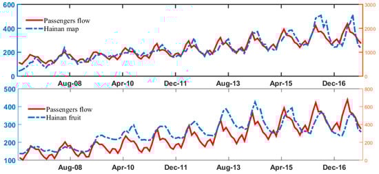
Figure 3.
Trend diagram between the “Hainan map” as well as the “Hainan fruit” and predicted variables.
The correlation analysis between all the predictive variables and the predicted variables in the experimental dataset is listed in Table 1. It can be seen that the lag order of the keyword predictive variables obtained by the cross-correlation analysis was 0–5, most of them were 0–1, and these variables had a significant correlation with the predicted variables, which fully reflected the potential tourism demands of tourists. For example, tourists inquired about travel guides, weather, maps and scenic spots information about one month in advance. Considering the periodic nonlinear characteristics of the forecasted variable and the excellent predictive ability of LSTM for the complex time series, it was assumed that the selected keyword variable as the input set of LSTM can effectively forecast the overnight passengers flow of tourist hotels. According to step 4 in the forecasting framework, the standardized dataset finally used in this paper can be expressed as follows:
Each of which contains 125 observations, where, refer to the predictive variables, and refers to the predicted variable. Each variable is aligned according to the lag order. The first 113 sample points in the experimental dataset were used for training, and the last 12 months of data were used for the testing.

Table 1.
Correlation analysis of the predictive variable.
4.2. Benchmark Models and Experimental Setup
For the purpose of confirming the forecasting power of the LSTM network under the forecasting framework, DBN, BPNN and the C-LSTM models were constructed as benchmark counterparts. Among them, DBN was a non-convolution architecture using deep framework training successfully [38], which was essentially a generation network. DBN was introduced to illustrate the advantages of LSTM in the complex time series forecasting. BPNN is a shallow learning method with only one hidden layer. It is a FFNN model and adds a BP algorithm to the structure of the feed-forward network. The introduction of BPNN was aimed to compare the forecasting ability of the DL technology with that of shallow learning methods. C-LSTM however, used only the historical data of the predicted variables as the model inputs, which was introduced to further confirm the importance of the Internet search data.
In terms of the experimental setup, to solve the phenomenon of over-fitting, the randomization selection rate of Dropout for the hidden layer was set to 0.5 for regularization [34]. For the purpose of compromising between the complexity of model training and the local optimal solution, according to the recommendations of Hinton et al. (2012), the initialization learning rate of all models was set to one. BPNN used the classical gradient descent algorithm (GDA) to optimize parameters, and the other forecasting tools used the RMSProp for an iterative updating of the parameters [34]. Taking into account a fewer experimental dataset, the batch size was set to four. In terms of the activation function, tanh was utilized as the activation function of all layers in the BPNN. In addition to the default activation function of the model, the other three models used the tanh function as the activation function of all layers. For the purpose of ensuring the convergence of the loss function RMSE when iteration was stopped during the model training process, epoch was set to 150. Except that the BPNN was a shallow learning model with only one hidden unit, the rest were the DL network architecture with three hidden units.
4.3. Empirical Results and Discussion
According to step 5 of the forecasting framework, the training experiment was conducted on the training dataset, the optimal architecture after training was used as the predictive model to perform the predictive test. The prediction outcomes of the various models on the testing dataset are displayed in Table 2. The monthly optimal forecasting values are shown in bold. For the 12-month forecasting results, LSTM performed the best. The optimal forecasting results of LSTM, DBN, BPNN and C-LSTM were five, four, two and one month, respectively. Figure 4 demonstrates the forecasting curve of each model on the test dataset more intuitively. Overall, LSTM better fits the dynamic characteristics of the passenger flow whereas, the C-LSTM performs the worst, and all the benchmark models had a slightly poor fit performance in the last five months. The specific predictive power of each network is yet to be analyzed from the statistical indicators.
Table 2.
Predictive results of each model.
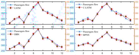
Figure 4.
Comparison of the fitting curves of the various models.
To further explore the predictive power of our proposed method, the statistic scores calculated on the experimental dataset are shown in Table 3, and the best score for each metric indicator was indicated in bold. In general, in addition to PBIAS, LSTM exhibited best on the scores of the other metric indicators. It is worth noting that the predictive accuracy of LSTM and DBN on the test set was better or very close to that of the training section, but the other three models are just the opposite, which suggests LSTM and DBN had a better generalization performance.
Table 3.
Metric indicator scores for each model on the experimental dataset.
On the testing dataset, the LSTM score was the smallest and the C-LSTM score was the highest in terms of the RMSE and MRE indicators, indicating that the deviation between the predicted record and the actual observation of LSTM was smaller with a better predictive accuracy than the benchmark models while, C-LSTM had the worst predictive accuracy. In terms of the goodness-of-fit indicator R, four models performed very close, and can fit the passengers flow well, but the fitting effects of LSTM and C-LSTM were the best and worst, respectively. In terms of PBIAS, the scores of all the models were small and all the score ranking were “excellent” [39]. However, C-LSTM and DBN performed better, while BPNN exhibited the worst. Except that BPNN underestimated the actual value on an average, the other three models overestimated the actual value on average.
4.4. Predictive Accuracy Test among Groups
In order to determine whether there exists a sharp distinction in the predictive accuracy between LSTM and its counterparts, the percent error of each network was applied for the t-test, where and represented the actual passenger flows and the predicted values, respectively. The essence of the t-test was to confirm whether the average value of the predictive accuracy between the developed network and each benchmark counterpart was equal. The following statistical assumptions were made:
Hypothesis 0 (H0).
There is no difference in the predictive accuracy between LSTM and the benchmark model.
Hypothesis 1 (H1).
The predictive accuracy between LSTM and its competitor model is not equal.
The testing outcomes are illustrated in Table 4. As seen from the table, the 10% significance level rejects the hypothesis that the predictive accuracy between LSTM and DBN is equal; while for LSTM, C-LSTM and BPNN, the 5% significance level rejects the null hypothesis. This implies that there exists an obvious distinction in the predictive accuracy between the constructed method and its competitors.
Table 4.
Test of significance between LSTM and its competitors.
In general, because the LSTM model can detect and learn the long-time dynamic information of the time series, it produces minimum error rate for the monthly passengers flow with periodic fluctuation characteristics, which agree with the conclusions of Aggarwal and Aggarwal [24] as well as Heaton et al. [40]. As C-LSTM failed to utilize the consumer query index as its inputs, its predictive accuracy was obviously different from that of LSTM at a 5% level of significance, and the error rate MAPE on the test section increased by 27.303%, which fully proved that the addition of the search query data drastically improved the forecasting performance of the models thereby, further confirming the conclusions of Zhang et al. [5] and Law et al. [25]. BPNN had a poor predictive ability due to its difference in the model structure from the DL method. Due to the disadvantages of the DBN in learning and storing long-term information, the learning ability of DBN was slightly worse than that of LSTM, and the predictive accuracy was slightly different at the 10% level of significance.
5. Conclusions
Hotel accommodation demands exhibit a cyclical fluctuation and complex nonlinear characteristics. Considering that the traditional prediction techniques cannot meet the ever-increasing data samples, and unable to automatically extract feature information, a forecasting framework based on DL was constructed in this paper. Taking Hainan in China as an empirical example, the LSTM model with a good predictive power for the complex time series was developed, and the Internet query index was used as the model inputs to forecast the overnight passengers flow of tourist hotels. The experimental outcomes implied that as compared to the benchmark models, LSTM improved the model predictive ability to different degrees, displayed satisfactory prediction ability and powerful generalization, and can simulate the dynamic characteristics of the passenger flow as well.
The preferable forecast performance can be attributed to the following three aspects. Firstly, additional memory units and special network structures enable the LSTM to learn the complex dynamic information of the passengers flow time series with a relatively large sample. Therefore, as compared to the DBN model, the LSTM model can learn the characteristic information of the passenger flows, which obviously improves the predictive ability of the model. Secondly, with the advent of the Internet environment, the consumer’s information query objectively reflects the potential demands for travel, and can forecast the trend of the overnight passenger flows of tourist hotels in advance. Therefore, the incorporation of the network query index makes the LSTM model better fit the dynamics of the overnight passenger flow in tourist hotels, and significantly improves the predictive performance of the developed LSTM network, which agree with the theoretical analysis. Finally, different optimization algorithms and a special network structure design make the learning ability and predictive ability of the LSTM significantly different from that of BPNN.
The research in this paper has a prominent theoretical significance. Firstly, an empirical framework based on web queries was constructed for the ever-growing sample of tourism data. Secondly, the LSTM deep learning model was introduced for the first time to forecast the hotel accommodation demands, extending the application of DL methods in hotel demand forecasting. Finally, it is confirmed that LSTM can simulate the relationship between the Internet queries and the tourism demands of hotels. This breaks through the limitations of the traditional forecasting technology and provides a typical application case for the deep integration of tourism data with a relatively large dataset, artificial intelligence and real economy.
As far as applications are concerned, the constructed forecasting framework provides a new solution for the hotel accommodation demand forecasting done by managers of tourism-related departments under the Internet environment, which helps tourism-related departments to dynamically monitor the hotel overnights; it provides decision support for realizing the information of the destination management. In addition, the constructed empirical framework can be used to forecast other destination demands such as hotel revenues, etc. It can further be extended to other similar prediction fields.
Nevertheless, in the context of the voluminous data, there may be other characteristic information that may reflect the tourists’ potential tourism demands. In future research, it is necessary to further expand other sources of information reflecting the dynamic characteristics of the hotel accommodation demands. In addition, the volume of the available sample data collection limits the research results. As the data sample further increases, the validity of the empirical framework can be tested by the actual cases.
Author Contributions
Conceptualization, B.Z.; formal analysis, Y.P.; methodology, B.Z.; project administration, J.L.; software, B.Z. and Y.P.; visualization, Y.W. and J.L.; writing—original draft, B.Z.; writing—review & editing, Y.P., Y.W. and J.L.
Funding
This research received no external funding.
Acknowledgments
This work was jointly supported by grants from the Chongqing Social Science Planning of China under grant No. 2017YBGL137, and a funding project for the Science and Technology Research Program of Chongqing Municipal Education Commission of China under grant No. KJQN201800520. The authors are grateful to the editors and the anonymous reviewers for their valuable comments and suggestions.
Conflicts of Interest
The authors declare no conflict of interest.
References
- Weatherford, L.R.; Kimes, S.E. A comparison of forecasting methods for hotel revenue management. Int. J. Forecast. 2003, 19, 401–415. [Google Scholar] [CrossRef]
- Song, H.; Li, G. Tourism demand modelling and forecasting—A review of recent research. Tour. Manag. 2008, 29, 203–220. [Google Scholar] [CrossRef]
- Li, X.; Pan, B.; Law, R.; Huang, X. Forecasting tourism demand with composite search index. Tour. Manag. 2017, 59, 57–66. [Google Scholar] [CrossRef]
- Chen, R.; Liang, C.R.; Hong, W.C.; Gu, D.X. Forecasting holiday daily passenger flow based on seasonal support vector regression with adaptive genetic algorithm. Appl. Soft Comput. 2015, 26, 435–443. [Google Scholar] [CrossRef]
- Zhang, B.; Huang, X.; Li, N.; Law, R. A novel hybrid model for tourist volume forecasting incorporating search engine data. Asia Pac. J. Tour. Res. 2017, 2, 245–254. [Google Scholar] [CrossRef]
- Sun, S.; Wei, Y.; Tsui, K.L.; Wang, S. Forecasting tourist arrivals with machine learning and internet search index. Tour. Manag. 2019, 70, 4165–4169. [Google Scholar] [CrossRef]
- Pan, B.; Fesenmaier, D.R. Online information search: Vacation planning process. Ann. Tour. Res. 2006, 3, 809–832. [Google Scholar] [CrossRef]
- Fesenmaier, D.R.; Cook, S.D.; Zach, F.; Gretzel, U.; Stienmetz, J. Travelers’ Use of Theinternet; Travel Industry Association of America: Washington, DC, USA, 2009. [Google Scholar]
- Choi, H.; Varian, H. Predicting present with Google trends. Econ. Rec. 2012, 88, 2–9. [Google Scholar] [CrossRef]
- Yang, Y.; Pan, B.; Song, H. Predicting hotel demand using destination marketingorganization’s Network traffic data. J. Travel Res. 2014, 53, 433–447. [Google Scholar] [CrossRef]
- Yang, X.; Pan, B.; James, A.; Lv, B. Forecasting Chinese tourists volume with search engine data. Tour. Manag. 2015, 46, 386–397. [Google Scholar] [CrossRef]
- Huang, X.; Zhang, L.; Ding, Y. The Baidu Index: Uses in predicting tourism flows–A case study of the Forbidden City. Tour. Manag. 2017, 58, 301–306. [Google Scholar] [CrossRef]
- Wei, J.R.; Cui, H.M. The Construction of Regional Tourism Index and Its Micro-Dynamic Characteristics: A Case Study of Xi’an. J. Syst. Sci. Complex. 2018, 38, 177–194. [Google Scholar]
- Li, S.; Chen, T.; Wang, L.; Ming, C. Effective tourist volume forecasting supported by PCA and improved BPNN using Baidu index. Tour. Manag. 2018, 68, 116–126. [Google Scholar] [CrossRef]
- Andrew, W.P.; Cranage, D.A.; Lee, C.K. Forecasting hotel occupancy rates with time series models: An empirical analysis. Hosp. Res. J. 1990, 14, 173–182. [Google Scholar] [CrossRef]
- Schwartz, Z.; Hiemstra, S. Improving the accuracy of hotel reservations forecasting: Curves similarity approach. J. Travel Res. 1997, 36, 3–14. [Google Scholar] [CrossRef]
- Pfeifer, P.E.; Bodily, S.E. A test of space-time arma modelling and forecasting of hotel data. J. Forecast. 1990, 9, 255–272. [Google Scholar] [CrossRef]
- Choi, J.G. Developing an economic indicator system (a forecasting technique) for the hotel industry. Int. J. Hosp. Manag. 2003, 2, 147–159. [Google Scholar] [CrossRef]
- Aliyev, R.; Salehi, S.; Aliyev, R. Development of fuzzy time series model for hotel occupancy forecasting. Sustainability 2019, 11, 793. [Google Scholar] [CrossRef]
- Pan, B.; Chenguang Wu, D.; Song, H. Forecasting hotel room demand using search engine data. J. Hosp. Tour. Technol. 2012, 3, 196–210. [Google Scholar] [CrossRef]
- LeCun, Y.; Bengio, Y.; Hinton, G. Deep learning. Nature 2015, 521, 436–444. [Google Scholar] [CrossRef]
- Zhu, X.; Vondrick, C.; Fowlkes, C.C.; Ramanan, D. Do we need more training data? Int. J. Comput. Vis. 2016, 119, 76–92. [Google Scholar] [CrossRef]
- Hochreiter, S.; Schmidhuber, J. Long short-term memory. Neural Comput. 1997, 9, 1735–1780. [Google Scholar] [CrossRef]
- Aggarwal, S.; Aggarwal, S. Deep Investment in financial markets using deep learningmodels. Int. J. Comput. Appl. 2017, 162, 40–43. [Google Scholar]
- Law, R.; Li, G.; Fong, D.K.C.; Han, X. Tourism demand forecasting: A deep learning approach. Ann. Tour. Res. 2019, 75, 410–423. [Google Scholar] [CrossRef]
- Chang, Y.W.; Tsai, C.Y. Apply deep learning neural network to forecast number of tourists. In Proceedings of the IEEE International Conference on Advanced Information Networking and Applications Workshops, Taipei, Taiwan, 27–29 March 2017; pp. 259–264. [Google Scholar]
- Gnoth, J. Tourism motivation and expectation formation. Ann. Tour. Res. 1997, 24, 283–304. [Google Scholar] [CrossRef]
- Pearce, P.L. Tourist Behaviour and the Contemporary World; Channel View Publications: Bristol, UK, 2011. [Google Scholar]
- Vila, T.D.; Vila, N.A.; Alén González, E.; Brea, J.A.F. The role of the internet as a tool to search for tourist information. J. Glob. Inf. Manag. 2018, 26, 58–84. [Google Scholar] [CrossRef]
- Jeng, J.; Fesenmaier, D.R. Conceptualizing the travel decision-making hierarchy: A review of recent developments. Tour. Anal. 2002, 7, 15–32. [Google Scholar] [CrossRef]
- Dean, J.; Corrado, G.S.; Monga, R.; Chen, K.; Ng, A.Y. Large Scale Distributed Deep Networks; Advances in Neural Information Processing Systems: Vancouver, BC, Canada, 2012; pp. 1223–1231. [Google Scholar]
- Lake, B.M.; Salakhutdinov, R.; Tenenbaum, J.B. Human-level concept learning through probabilistic program induction. Science 2015, 350, 1332–1338. [Google Scholar] [CrossRef]
- Goodfellow, I.; Bengio, Y.; Courville, A. Deep Learning; MIT Press: Cambridge, MA, USA, 2017. [Google Scholar]
- Hinton, G.; Deng, L.; Dong, Y.; Dahl, G.E.; Mohamed, A.; Jaitly, N.; Senior, A.; Vanhoucke, V.; Nguyen, P.; Sainath, T.N. Deep neural networks for acoustic modelling in speech recognition: The shared views of four research groups. IEEE Signal Process. Mag. 2012, 29, 82–97. [Google Scholar] [CrossRef]
- Chollet, K. Keras. Available online: https://github.com/fchollet/keras.2015 (accessed on 5 September 2017).
- Hadavandi, E.; Shavandi, H.; Ghanbari, A.; Abbasian-Naghneh, S. Developing a hybrid artificial intelligence model for outpatient visits forecasting in hospitals. Appl. Soft Comput. 2012, 12, 700–711. [Google Scholar] [CrossRef]
- Gupta, H.V.; Sorooshian, S.; Yapo, P.O. Status of automatic calibration for hydrologic models: Comparison with multilevel expert calibration. J. Hydrol. Eng. 1999, 4, 135–143. [Google Scholar] [CrossRef]
- Hinton, G.E.; Osindero, S.; Teh, Y. A fast learning algorithm for deep belief nets. Neural Comput. 2006, 18, 1527–1554. [Google Scholar] [CrossRef] [PubMed]
- Moriasi, D.N.; Arnold, J.G.; Liew, M.W.V.; Bingner, R.L.; Harmel, R.D.; Veith, T.L. Model evaluation guidelines for systematic quantification of accuracy in watershed simulations. Trans. ASABE 2007, 50, 885–900. [Google Scholar] [CrossRef]
- Heaton, J.B.; Polson, N.G.; Witte, J.H. Deep Learning in Finance. Working Paper. Available online: https://arxiv.org/pdf/1602.06561.pdf (accessed on 10 April 2018).
© 2019 by the authors. Licensee MDPI, Basel, Switzerland. This article is an open access article distributed under the terms and conditions of the Creative Commons Attribution (CC BY) license (http://creativecommons.org/licenses/by/4.0/).