Modeling of the Relationship Between Speed Limit and Characteristic Speed of Expressway Traffic Flow

Abstract

Understanding the relationship between speed limit and characteristic speed of expressway traffic flow is of great significance for formulating a reasonable speed limit scheme and improving highway safety and transportation efficiency. In this study, the speed data of the same traffic flow passing through speed limits of 80, 100, and 120 km/h were continuously collected through a field test. The 85th, 15th, and 50th percentile speeds were considered the characteristic speed parameters of the traffic flow. A regression analysis was performed to establish a relationship between the characteristic speed parameters of the traffic flow and the speed limit. Under a free-flow state, the characteristic speed exhibited a strong linear relationship with the speed limit, where the variation ranges of the 85th and 50th percentile speeds were approximately consistent with that of the speed limit. However, a slight inconsistency was found for the 15th percentile speed, which was approximately half the speed limit increase; under a non-free-flow state, the correlation between the speed limit and the vehicle speed was no longer significant.

1. Introduction

The speed limit and the operating speed have a strong correlation. Before setting the speed limit, the change in the actual operating speed of vehicles should be considered [1]. Any change in the speed limit will lead to changes in the speed of traffic flow [2]. Most conventional speed limit setting methods are based on the design speed, and the operating speed is not fully considered [3,4]. Such a speed limit scheme does not meet the speed expectations of drivers. As a result, the operational efficiency of expressways is generally low, and the driving safety is significantly affected. With the development of technology, people are increasingly demanding travel efficiency. Reasonably increasing the speed limit is a common request by drivers [5]. However, the effects of increasing the speed limit on the operational efficiency of expressways and road safety remain unclear. The above problems can be explained based on the speed of traffic flow at a micro level [3,6,7,8]. Therefore, it is of great practical significance to study the relationship between the speed limit and the characteristic speed of expressway traffic flow.

The percentile speed is an important factor that helps understand the characteristics of traffic flow: The 85th percentile speed characterizes speed changes greater than 85% of the traffic flow, using to indicate the overall operating speed. The 15th percentile speed indicates the speed characteristics of less than 15% of the traffic flow and can be used as a basis for setting the minimum speed limit. The 50th percentile speed reflects the efficiency of road operations [3,6,7,8]. Taking 85th, 15th, and 50th percentile speeds as the parameters of the characteristic velocity of traffic flow, we analyzed the influence of the speed limit on each parameter in this study.

Related research mainly focused on the relationship between design speed, operating speed, and speed limit, with some generally accepted or fully demonstrated results and conclusions [9,10,11,12,13,14,15]. To predict the running speed of vehicles on roads, Fitzpatrick considered the speed limit as the only factor affecting the running speed and established a predictive model for general roads: EV85 = 7.657 + 0.98PSL (PSL means posted speed limit) [16,17,18]. Winsor et al. studied the traffic flow law after the speed limit in USA increased from 55 to 65 mph in 1987 by collecting speed and safety data before and after the speed limit change. A unified conclusion was drawn: when the speed limit increases, the speed in the free-flow state increases without any increase in the accident rate [19,20,21]. McLean studied the difference in the design speed and the speed of two-lane highways in Australia. The results showed that, for a flat curve with a design speed lower than 90 km/h, the 85th percentile speed is always higher than the design speed. However, for a flat curve with a design speed higher than 90 km/h, the 85th percentile speed is always lower than the design speed [22]. Studies have also been conducted on the influence of the characteristic speed of traffic flow on the setting of the speed limit value and the rationality of the speed limit setting. Parker conducted a survey for state traffic management departments in the United States and argued that the 85th percentile speed is the most significant factor in determining the speed limit. The state traffic management departments can use the 85th percentile speed as an important basis for adjusting the speed limit plan [23]. The American Institute of Transportation Engineers believes that the speed limit must be determined in accordance with the driving conditions of vehicles. The speed limit should be approximately 8 km/h higher than the 85th percentile speed; thus, when a vehicle is running, the speed variance will be maintained in a small range, and the vehicle will be safer and more stable [24].

In summary, scholars have studied the relationship between the speed limit, design speed, and operating speed; however, the starting point should be to verify the rationality of the speed limit instead of the speed limit setting. Currently, there is a lack of systematic discussion on the relationship between the speed limit and the 85th, 15th, and 50th percentile speeds. Although some studies have been conducted, there have been no convincing conclusions because of the small number of research samples or the unreasonable selection of locations. Therefore, we selected sections with the same vertical slope, flat curve radius, and cross-section on the same expressway, with three speed limiting schemes (80, 100, and 120 km/h). The speed and traffic volume data of the traffic flow were analyzed using a sufficient sample size under the three speed limit values. The 85th, 15th, and 50th percentile speeds were taken as the characteristic velocity parameters of the traffic flow. The relationship between the speed limit and the speed parameters of each characteristic traffic flow was determined through mathematical and statistical analyses, providing a technical reference for rationally determining a speed limit scheme under different traffic flow conditions.

2. Methodology

Many factors affect the speed of highway traffic flow. In addition to the speed limit, the road alignment, environmental lateral disturbance, traffic flow density, and driving behavior are influencing factors. To determine the relationship between different speed limits and the characteristic speed of expressway traffic flow, the other influencing factors should be strictly controlled. During the test, the speed limit change should be the only factor affecting the speed of traffic flow. Considering the limitations of the test conditions, such as the uncontrollability of traffic flow density, the traffic flow will gradually change over time. In this paper, v/C is introduced to describe the state of road traffic flow as an intermediate variable between the speed limit and the characteristic speed parameters of traffic flow. According to the Design Specification for Highway Alignment of China [25], the traffic flow at the primary service level (v/C ≤ 0.35) is in a completely free-flow state; the traffic flow at the secondary service level (0.35 < v/C ≤ 0.55) is in a relatively free-flow state, and the driver can choose the driving speed according to his/her own wish. The measured test data reflect the normal trend in driving; when v/C > 0.55, the traffic flow enters a saturated state, and the flow is congested. Under this condition, the vehicles significantly affect each other, forming a queue flow.

We collected the speed data from real vehicles by conducting tests. The v/C values of each set of data were calculated [25] using Equation (1). The benchmark capacity is the maximum service traffic volume corresponding to the five-level service.

$$\frac{v}{C}=\frac{Maximum service traffic volume}{Benchmark capacity}$$

(1)

The percentile speed of each set of data was derived using IBM SPSS Statistics software. A direct relationship model between the speed limit and the traffic flow characteristic speed was established by conducting a regression analysis. According to previous studies, it is assumed that the speed limit has a linear regression relationship with the 85th, 15th, and 50th percentile speeds. This relationship is expressed using Equation (2):

$$EV85\left(EV50,EV15\right)=\mathrm{a}\times \mathrm{PSL}+\mathrm{b}$$

(2)

Here, both a and b are fixed constants. To verify the above hypothesis, tests were conducted to collect data.

2.1. Test Plan

To eliminate the interference of the road line shape, environment, and other factors on the test data, in the test, the following test control was carried out in this study:

(1) To eliminate the influence of road line shape on the vehicle speed in the test section, when selecting the test section, the linear curve parameters, such as the flat curve radius and the longitudinal slope, should be consistent at each speed limit point. Therefore, the test section is designated as the straight section of K912+000-K903+800 after the Nanwutai Tunnel of the Ankang-Xi’an section of the Xikang Expressway, as listed in

Table 1. Operating speed collection location

Measuring Station	Test Location
Xikang Expressway Ankang to Xi’an Section K910+500	About 1200 m after the 80 km/h speed limit sign
Xikang Expressway Ankang to Xi’an Section K909+60	About 800 m after the 100 km/h speed limit sign
Xikang Expressway Ankang to Xi’an Section K903+800	About 1100 m after the 120 km/h speed limit sign

. The road section has a good line shape, the speed limit setting is reasonable, and the management is strict. Therefore, the speed data of this section are more objective. There are three measuring points in the test. The measuring points are respectively arranged at a distance after the speed limit marks of 80, 100, and 120 km/h. Thus, the speed characteristics of each speed limit segment after the speed is stabilized can be collected. Figure 1 shows the schematic of the test scheme.

(2) To eliminate the impact of environment on the operation of the test section, we strictly controlled the test time: During the test, the weather conditions were good, the wind was low, the visibility was high, and the road surface was dry without any water.

(3) To consider the influence of different traffic flow density on the speed at the measuring point, before the test, we requested the management department ensure that the traffic volume of the test section is within a v/C range of 0–0.55. This includes the full state of the free-flow measurement peak, the middle peak, and the low peak of the traffic flow. This type of traffic volume can comprehensively describe the relationship between the speed limit and the characteristic speed under different traffic flow conditions.

Moreover, to ensure a sufficient sample size, the velocity was determined in units of 30 min to ensure that the sample size satisfies the allowable error of 2 km/h and the minimum sample size calculated by the 98% confidence level.

(4) To eliminate the influence of the test instrument and the tester on the driving behavior as much as possible and to ensure the authenticity of the collected speed data, a Nanolaser (roadside laser vehicle classification statistical system) roadside instrument was employed as the test equipment, as shown in Figure 2. This instrument can automatically collect the vehicle speed characteristics. Compared with the conventional speed measuring instruments, the Nanolaser roadside instrument has the following advantages: (1) It has a small volume and can be placed on the outermost edge of a hard shoulder. The instrument generally does not attract the attention of the driver, and the concealability is high when collecting the speed data; (2) The instrument uses a laser sensing method to collect parameters, such as the vehicle speed and vehicle type, and is suitable for speed collection under various traffic flow states. The collected data are more accurate.

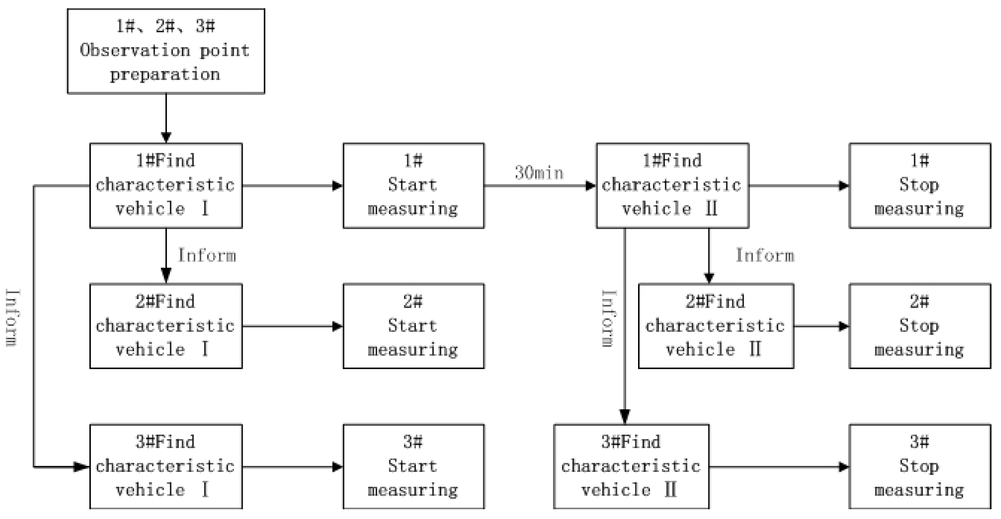
The specific test plan is as follows: Two speed measuring personnel are sent to each measuring point during the test. Before the test begins, the tester arrives at the speed measuring point to set up and debug the road tester to ensure that the instrument collection results are correct and normal. After the preparation of the three sets of measuring points, the first group of testers selects the characteristic vehicle and conveys its characteristics and license plate number to the second and third groups. The three groups measure the speed after seeing the characteristic vehicle. At the end, the characteristic vehicle is also selected to ensure that the three test groups collect the same traffic data. Figure 3 shows a flowchart of the specific process. This cycle is continued until the total sample traffic volume covers the traffic flow. In the field test, the tester should be hidden to avoid any objective effect of the test on the driving behavior.

2.2. Data Preprocessing

Because of the long collection time of the test, it is necessary to check and save the collected raw speed data in time. In this process, we found individual anomalies in the data. To eliminate the data error due to the instrument, the abnormal data were eliminated as follows:

(1) Speed less than 30 km/h: This happens because the vehicle is temporarily parked near the roadside instrument and should be deleted during data preprocessing.

(2) Speed greater than 160 km/h: This situation occurs because the vehicle is accidentally detected by the instrument when the roadside instrument is affected by dust. This should be deleted when the data are preprocessed.

(3) Vehicle model shows pedestrians or motorcycles and electric vehicles. The reason for this is that some pedestrians or non-motor vehicles are on the road. This should be deleted when data are preprocessed.

3. Results

3.1. Relationship Between Speed Limit and 85th Percentile Speed

In this test, a total of 87 sets of traffic flow velocity data under different v/C and free=flow states were collected. Each set of data was collected in units of 30 min, and the data met the minimum sample size and the normal distribution test. The data eliminated during data preprocessing accounted for 0.375% of the total data; this does not affect the accuracy. The valid data are imported to the IBM SPSS Statistics software, and the traffic flow characteristic speed parameters for each set of data are outputted. With v/C as the intermediate variable, the relationship between the characteristic velocity parameter and v/C is first established, and the variation law of traffic flow characteristic velocity under different traffic flow conditions is analyzed. A direct relationship model between the speed limit and the feature speed is established by fixing v/C. 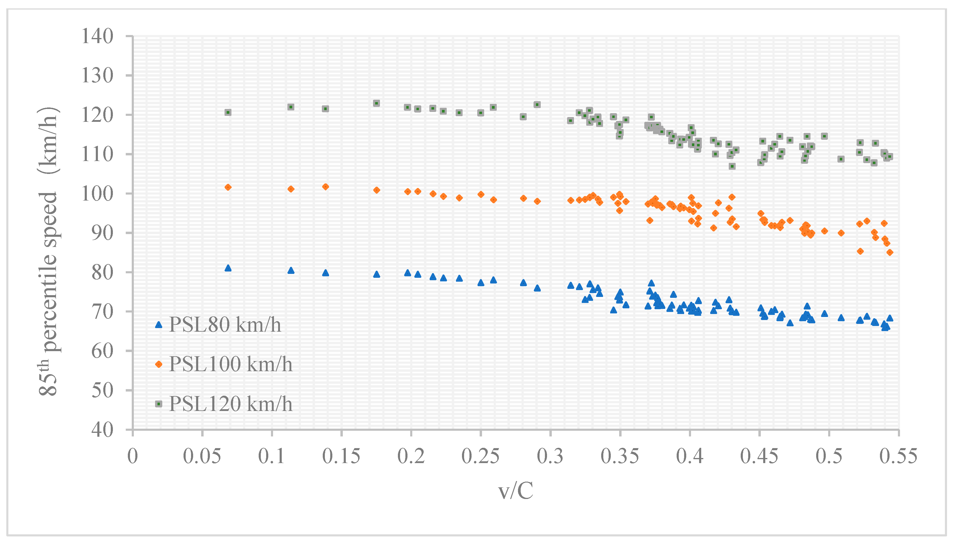Figure 4 shows the scatter plot of the relationship between the 85th percentile speed and v/C.

As the characteristic speed parameters, such as the 85th and 15th percentile speeds, are required to evaluate the operating speed characteristics of the traffic flow in the free-flow state, the range of the established horizontal scatter plot v/C is taken as 0–0.55. As shown in Figure 4, the vehicle operating speed has a strong correlation with v/C. As v/C increases, the operating speed gradually decreases. The trend line must be fitted through the scatter plot to find the exact relationship between the average operating speed and v/C. Combining relevant research and traffic flow theory, it is found that there is a strong linear relationship between the operating speed and v/C. 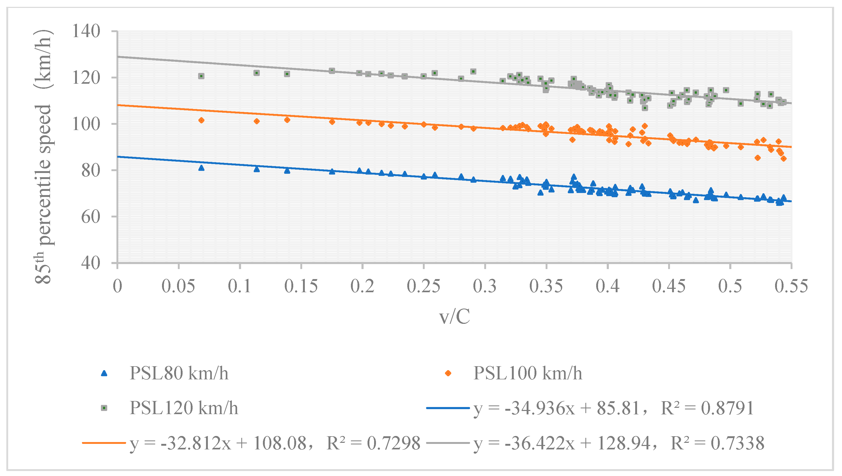Therefore, we obtained a linear fit to the scatter plot, as shown in Figure 5.

In Figure 5, the solid line part indicates the scatter fitting trend line of the 85th percentile speed and v/C, and R2 is the fitting coefficient of each trend line. The figure shows that, under the three speed limits, the fitting coefficient of each trend line is approximately 0.8. This shows that there is a strong linear relationship between the two. The accuracy of the model is high, and it can reflect the characteristics of the vehicle speed change under different traffic flow in the test section. In the figure, we find that the v/C data are mostly concentrated in the range of 0.25–0.55, and the data in the range of 0–0.25 are relatively less. This is because, when v/C is in the range of 0–0.25, the data were measured mostly late at night, and vehicles during this time are fewer. Because of driver fatigue and line-of-sight, the characteristic speed of the actual running vehicle is concentrated below the trend line.

In addition, the slopes of the three trend lines are largely the same, and the increase in the intercept is the same as the increase in the speed limit. It is found that the increment of the 85th percentile speed in different speed limitation is almost irrelevant with v/C. To find out the direct relationship between speed limit and the 85th percentile speed, we divided v/C into groups of 0.05 units to control the effect of traffic volume on the vehicle speed. The average running speed of each group is determined, and a relationship between the 85th percentile speed and the speed limit is established, as shown in Figure 6.

Figure 6 shows that. under the free-flow state, the speed limit is linearly related to the operating speed of the vehicle, and the fitting coefficient is as high as 0.9412. As the speed limit increases, the 85th percentile speed increases linearly. The slope of 1.0381 indicates that, the growth rate is the same as the rate limit increase: for every 20 km/h increase in the speed limit, the 85th percentile speed increases by approximately 20 km/h. This shows that the speed limit has a greater constraint on the operating speed of the vehicle, and most drivers will adjust the speed according to the speed limit value. A relationship model between the 85th percentile speed and the speed limit value is established using Equation (3).

$$\mathrm{EV}85=1.0381\mathrm{PSL}-6.9038,R^2=0.9412,PSL\in \left[80km/h,120km/h\right]$$

(3)

Equation (3) shows that the speed limit has a significant effect on the 85th percentile speed: When the speed limit is in the range of 80–120 km/h, the average operating speed varies linearly with the change in the speed limit. The fitting coefficient of the model is up to 0.9412, and the average operating speed is below the speed limit. This model can be used to calculate the 85th percentile speed at different speed limits, thus playing an important role in the safety estimation following an increase in the road speed.

3.2. Relationship Between Speed Limit and 15th and 50th Percentile Speeds

Using the above method to study the effect of speed limit on the 15th and 50th percentile speeds, we determined the relationship between the 15th percentile speed and v/C in the free-flow state, as shown in Figure 7.

As shown in Figure 7, the 15th percentile speed is also linearly related to v/C. However, the increase in the 15th percentile speed is not consistent with the increase in the speed limit; it is approximately half the speed limit increase. This may be because the driving speed is significantly affected by the driver’s traits. Some drivers can be affected by their driving level and/or driving experience. They are not sensitive to the speed limit when driving on expressways, resulting in a low driving speed and driving behaviors that do not meet the requirements of expressway management departments. In addition, the 15th percentile speed at a speed limit of 120 km/h is approximately 90 km/h. This shows that when the vehicle is being driven at a high speed limit, about 15% of the vehicles will be driven at a speed lower than the speed limit value of 30 km/h. This increases the traffic flow speed of the highway, thus leading to safety issues.

The same method is applied to analyze the influence of the speed limit on the 15th percentile speed. The relevant models are established:

$$\mathrm{EV}15=0.693\mathrm{PSL}+4.436,R^2=0.8812,PSL\in \left[80km/h,120km/h\right]$$

(4)

According to Equation (4), the speed limit has a significant effect on the 15th percentile speed: when the speed limit value is in the range of 80–120 km/h, the average 15th percentile speed varies linearly with the change in the speed limit. The fitting coefficient is also as high as 0.8812, indicating that the model has a high accuracy. With the relationship model between the speed limit and the average 15th percentile speed, it is possible to predict the 15th percentile speed at different speed limits and help highway management departments to comprehensively consider the setting of the speed limit by combining different driving characteristics.

A relationship between the 50th percentile speed and v/C under a free-flow state is established, as shown in Figure 8.

Figure 8 shows that the 50th percentile speed is linearly related to v/C in the free-flow state as well. For every 20 km/h increase in the speed limit, the average 50th percentile speed of the vehicle increases by approximately 18 km/h, which is the same as the increase in the speed limit, indicating that the speed limit in the free-flow state has a greater impact on the average 50th percentile speed of the vehicle. The 50th percentile speed can better describe the driving speed of drivers with a typical driving level. It reflects the running efficiency of the vehicle on the road. As shown in Figure 8, the average value of the 50th percentile speed is approximately 20 km/h lower than the maximum speed limit of the road. This shows that the operating efficiency of the test section did not meet the expectations, and the functional characteristics of this road were not fully exploited. A relationship model between the speed limit and the 50th percentile speed is established as follows:

$$\mathrm{EV}50=0.949\mathrm{PSL}-9.0965,R^2=0.8765,PSL\in \left[80km/h,120km/h\right]$$

(5)

Equation (5) can also better reflect the linear influence of the speed limit on V50, with the fitting coefficient reaching 0.8765. The model can better predict the average speed of the vehicle. This can help the highway manager to better understand the speed demand of drivers. The model can more reasonably determine the speed limit from the perspective of improving the operating efficiency.

3.3. Model Verification

Although the fitting coefficient R2 of the model is 0.9, to further verify the accuracy of the model, we continued to collect the velocity data from the test section after establishing the model. In addition to collecting the speed data under a free-flow state, data under a non-free-flow state were collected. We verified whether the characteristic speed parameter–speed limit model is applicable under a full traffic flow state. In the verification phase, the test plan was the same as before, and 20 sets of free-flow vehicle speed data and eight groups of non-free-flow speed data were collected. The effective data after removing the singular points accounted for 99.5% of the original data. To verify the accuracy of the model, the relative error was introduced to calculate the error between the measured and model calculation data. The calculation formula is as shown in Equation (6).

$$\mathrm{Relative}\mathrm{error}=\left|\frac{Measured value-Model calculated value}{Model calculated value}\right|\times 100\%$$

(6)

Table 2. Model relative error verification

v/C	PSL (km/h)	85th Percentile Speed Measured Value (km/h)	Relative Error	15th Percentile Speed Measured Value (km/h)	Relative Error	50th Percentile Speed Measured Value (km/h)	Relative Error
0.1386	80	79.848	4.86%	63.254	5.64%	72.388	8.33%
	100	101.688	4.93%	80.456	9.11%	90.838	5.87%
	120	121.46	3.22%	91.894	4.91%	112.256	7.13%
0.259	80	78.034	2.48%	61.28	2.34%	69.455	3.94%
	100	98.36	1.50%	75.142	1.91%	86.4	0.70%
	120	121.86	3.56%	90.456	3.26%	111.42	6.33%
0.3341	80	76.0154	0.17%	58.045	3.06%	66.92	0.14%
	100	98.5727	1.72%	75.4231	2.29%	85.95	0.17%
	120	119.355	1.43%	85.651	2.22%	106.65	1.78%
0.4303	80	70.124	7.91%	57.3725	4.18%	61.954	7.29%
	100	99.0485	2.21%	68.4213	7.21%	80.24	6.48%
	120	110.3598	6.21%	81.356	7.12%	100.92	3.69%
0.5271	80	68.776	9.68%	54.0805	9.68%	60.745	9.10%
	100	93.03	4.00%	67.267	8.77%	77.51	9.67%
	120	108.535	7.76%	78.862	9.97%	96.152	8.24%
0.6236	80	62.317	18.16%	51.145	14.58%	51.145	23.46%
	100	83.403	13.93%	66.48	9.84%	66.48	22.52%
	120	101.3592	13.86%	86.24	1.55%	86.24	17.70%
0.7514	80	49.034	35.60%	49.034	18.11%	49.034	26.62%
	100	60.45	37.62%	60.4523	18.02%	60.45	29.55%
	120	78.55	33.24%	78.5508	10.33%	78.55	25.04%

lists the relative error values of the characteristic parameters of the traffic flow for several representative v/C states.

Under a free-flow state, i.e., when v/C ≤ 0.55, the relative error values of the three characteristic speed parameter–speed limit models proposed in this paper are all below 10%, and most of them are below 5%. The accuracy of the model is quite high considering the dispersion of the vehicle speed due to different driver characteristics. In addition, the relative error of the model under a non-free-flow state is greater than 10%; the highest error is close to 40%. This shows that the accuracy of the model under non-free flow is not high. The is because the traffic flow density gradually increases, and the number of vehicles on the road gradually becomes saturated. This changes the factors affecting the driving speed and driving behavior. As a driver always pays attention to other users in traffic while driving, his/her driving freedom is affected. Under this condition, the factors affecting the driving speed are mainly changes in the external environment rather than the speed limit; this seriously affects the operating efficiency. In addition, the accuracy of the 15th percentile speed model under non-free flow is significantly higher than those of the 85th and 50th percentile speed models. This is due to driver characteristics and is consistent with the above analysis.

In summary, when traffic flow has a high density or is congested, it is recommended to use variable speed limiting means in the road section in front of the congested flow for a reasonable speed transition control of the traffic flow.

4. Discussion

In this study, the speed data of the same traffic flow passing through speed limits of 80, 100, and 120 km/h were collected in the field. The 85th, 15th, and 50th percentile speeds were used as the characteristic parameters of the traffic flow, and v/C was used as the intermediate quantity to characterize the traffic flow state. The relationship between the speed limit and the characteristic speed of expressway traffic flow was analyzed.

The results showed that, on the expressway, when the same traffic flow continuously passes through different speed limit values, the characteristic speed of the traffic flow and the speed limit change have a significant linear relationship. In the free-flow state (v/C ≤ 0.55), for every 20 km/h increase in the speed limit, both the 85th and 50th percentile speeds increase by approximately 20 km/h, and the increase in the 15th percentile speed is approximately 10 km/h. Based on the linear relationship model established in this paper, the influence of the characteristic speed of traffic flow on the speed limit variation of free-flow state expressways can be quantitatively analyzed when 80 km/h ≤ PSL ≤ 120 km/h.

The conclusions drawn from this study are consistent with those reached by Fitzpatrick, who studied the speed limit and traffic speed of two-lane highways in the United States [18]. This shows that the speed limit change significantly influences the traffic flow speed, and there is a strong positive correlation between the two. However, by further comparing the relational models, we find certain differences. In the model proposed by Fitzpatrick, the relationship between the speed limit of the general highway section and the running speed of the US highway satisfies the equation EV85 = 7.657 + 0.98PSL. In this study, the relationship between the two was found to be EV85 = 1.0381PSL - 6.9036. With regard to the specific speed limit calculation, the speed calculated using Fitzpatrick’s model is approximately 10 km/h higher than that established in this study. This is because, in the United States and Europe, it is generally believed that high-speed driving is important to maximize the operational efficiency of highways. The punishment for over-speeding is not strict, and a driver can basically select the driving speed according to the road conditions and his/her own expectations. On the contrary, in China, because of the large traffic volume on the road, the highway management departments are more strict, and the speed limit has a greater constraint on the driving of the vehicle. This results in a lower traffic speed compared with countries such as the United States. Therefore, the model established in this paper is more suitable for China, where the traffic volume is considerable and the speed limit strictly enforced.

In addition to the 85th percentile speed model, this study also establishes a linear model for the 50th and 15th percentile speeds and the speed limit. This can help highway managers to more accurately balance the relationship between operational efficiency and road safety through the traffic flow speed, i.e., by increasing the speed limit of the road or by changing the speed limit scheme, making the speed limit more in line with current requirements.

Because of the limitation of the test conditions, the traffic flow speed parameters were collected only under three speed limit standards (80, 100, and 120 km/h). The effect of other speed limit standards on the traffic flow speed should be further studied.

References

- The Institute of Engineers (ITE). Speed Zone Guidelines—A Proposed Recommended Practice; The Institute of Engineers: Washington, DC, USA, 1993. [Google Scholar]
- Himes, S.C.; Donnell, E.T.; Porter, R.J. Posted speed limit: To include or not to include in operating speed models. Transp. Res. Part A Policy Pract. 2013, 52, 23–33. [Google Scholar] [CrossRef]
- Technical Standards for Highway Engineering (JTG B01-2014); China Standard Press: Beijing, China, 2014.
- American Association of State Highway and Transportation Officials. A Policy on Geometric Design of Highways and Streets; American Association of State Highway and Transportation Officials: Washington, DC, USA, 2001. [Google Scholar]
- Lee, Y.M.; Chong, S.Y.; Goonting, K.; Sheppard, E. The effect of speed limit credibility on drivers’ speed choice. Transp. Res. Part F Traffic Psychol. Behav. 2017, 45, 43–53. [Google Scholar] [CrossRef]
- Transportation Research Board. Highway Capacity Manual; Transportation Research Board: Washington, DC, USA, 2016. [Google Scholar]
- Federal Highway Administration (FHWA). Speed Concepts: Informational Guide; Federal Highway Administration: McLean, VA, USA, 2009.
- World Health Organization. Speed Management: A Road Safety Manual for Decision-makers and Practitioners; Global Road Safety Partnership; World Health Organization: Geneva, Switzerland, 2008. [Google Scholar]
- Yao, Y.; Carsten, O.; Hibberd, D.; Li, P. Exploring the relationship between risk perception, speed limit credibility and speed limit compliance. Transp. Res. Part F Traffic Psychol. Behav. 2019, 62, 575–586. [Google Scholar] [CrossRef]
- Federal Highway Administration. Manual on Uniform Traffic Control Devices (MUTCD); Federal Highway Administration: Washington, DC, USA, 2003.
- Soriguera, F.; Martínez, I.; Sala, M.; Menéndez, M. Effects of low speed limits on freeway traffic flow. Transp. Res. Part C Emerg. Technol. 2017, 77, 257–274. [Google Scholar] [CrossRef]
- Hu, W. Raising the speed limit from 75 to 80 mph on Utah rural interstates: Effects on vehicle speeds and speed variance. J. Saf. Res. 2017, 61, 83–92. [Google Scholar] [CrossRef]
- Aljanahi, A.A.M.; Rhodes, A.H.; Metcalfe, A.V. Speed, Speed Limits and Road Traffic Accident Under Free Flow Conditions. Accid. Anal. Prev. 1999, 131, 161–168. [Google Scholar] [CrossRef]
- Dong, Y.; Xu, J.; Liu, X.; Gao, C.; Ru, H.; Duan, Z. Carbon Emissions and Expressway Traffic Flow Patterns in China. Sustainability 2019, 11, 2824. [Google Scholar] [CrossRef]
- Liu, X.; Xu, J.; Li, M.; Wei, L.; Ru, H. General-Logistic-Based Speed-Density Relationship Model Incorporating the Effect of Heavy Vehicles. Math. Probl. Eng. 2019, 2019, 1–10. [Google Scholar] [CrossRef]
- Fitzpatrick, K.; Blaschke, J.D.; Shamburger, C.B.; Krammes, R.A.; Fambro, D.B. Compatibility of Design Speed, Operating Speed, and Posted Speed; Texas Transportation Institute: College Station, TX, USA, 1995. [Google Scholar]
- Fitzpatrick, K. Is 85th Percentile Speed Used to Set Speed Limits? In ITE 2002 Annual Meeting and Exhibit; Institute of Transportation Engineers: Washington, DC, USA, 2002. [Google Scholar]
- Fitzpatrick, K. Predicting Operating Speeds on Tangent Sections of Two-Lane Rural Highways. Transp. Res. Rec. 2003, 1737, 50–57. [Google Scholar]
- Winsor, J. Fueling a debate: 55 mph vs. 65 mph in 1987. Diesel Prog. N. Am. Ed. 2004, 70, 4. [Google Scholar]
- Lave, C.; Elias, P. Did the 65 mph Speed Limit Save Lives? Accid. Anal. Prev. 1994, 26, 49–62. [Google Scholar] [CrossRef]
- Wagenaar, A.C.; Streff, F.M.; Schultz, R.H. Effects of the 65 mph speed limit on injury morbidity and mortality. Accid. Anal. Prev. 1990, 22, 571–585. [Google Scholar] [CrossRef]
- Kloeden, C.; Woolley, J.; McLean, A. Evaluation of the 50km/h Default Urban Speed Limit in South Australia; The University of Adelaide: Adelaide, Australia, 2004. [Google Scholar]
- Parker, M.R. Synthesis of Speed Zoning Practices, Report FHWA; U.S. Department of Transportation: Washington, DC, USA, 1985; p. 7.
- Taylor, W.C. Speed Zoning Guidelines: A Proposed Recommended Practice; Institute of Transportation Engineers: Washington, DC, USA, 1990. [Google Scholar]
- Design Specification for Highway Alignment of China Stipulates (JTG D21-2017); China Standard Press: Beijing, China, 2017.
© 2019 by the authors. Licensee MDPI, Basel, Switzerland. This article is an open access article distributed under the terms and conditions of the Creative Commons Attribution (CC BY) license (http://creativecommons.org/licenses/by/4.0/).