Comparison on Multi-Scale Urban Expansion Derived from Nightlight Imagery between China and India

Abstract

“The Dragon and the Elephant” between China and India is an important manifestation of global multipolarization in the 21st century. As engines of global economic growth, the two rising powers have followed similar courses of development but possess important differences in modes of development and urban development, which have attracted the widespread attention of scholars. From a geospatial perspective, and based on continuous annual night light data (Defense Meteorological Satellite Program-Operational Linescan System, DMSP-OLS) from 1992 to 2012, this paper conducts a multi-scale comparative analysis of urban development differences between China and India by employing various approaches such as the Gini coefficient, Getis–Ord Gi* index, and the Urban Expansion Intensity Index (UEII). The results show that: (1) The urban land space of the two countries expand rapidly, with the average annual expansion rate of China and India being 5.24% and 3.85%, respectively. The urban land expansion rate in China is 1.36 times faster than that in India. Resource-typed towns in arid northwest China and the resource-typed towns in central India have developed rapidly in recent years. (2) The unbalanced development in India is more prominent than in China; and the regional and provincial development imbalances in China are shrinking, while India’s imbalances are improving slowly and its regional differences are gradually widening. (3) The spatial pattern of land use in both countries shows significant coastal and inland differences. The difference between the east, the central regions, and the west is the main spatial pattern of China’s regional development, while the difference between the north and the south is the spatial pattern of India’s regional development. (4) There are obvious differences in the expansion intensity of core cities between the two countries. From 1997 to 2007, the expansion intensity of core cities in China was relatively higher than that in India, while that in India was relatively higher than that in China from 2007 to 2012.

1. Introduction

China and India are two rising world powers and are often referred to as “the driving force of Asia in global change“ [1]. To promote the rapid development of the economy, economic reforms and liberalization measures were implemented in China and India in 1978 and 1991, respectively. Since the implementation of reform and opening-up policy of China, the total GDP of China has increased from 0.15 trillion dollars in 1978 to 12.24 trillion dollars in 2017, with its world ranking having risen nine places during that period. Since the implementation of economic reforms in India, the total GDP has increased from 0.26 trillion dollars in 1991 to 2.6 trillion dollars in 2017, and its world ranking has risen by 10 places during that period. China and India have quickly developed into the world’s second and sixth largest economies by virtue of their successive accession to the World Trade Organization (WTO). However, India currently has a low urbanization rate, which increased from 25.72% in 1991 to 33.60% in 2017 [2], while China saw its urbanization rate increased from 17.92% in 1978 to 58.52% in 2017 [3]. The urbanization rate of the two countries differs by 24.92% with a population of about 350 million. Similar developmental histories and different developmental paths and models of China and India make their competition and development relations widely concerned.

In the 1980s, scholars from the United States, Japan, and the United Kingdom conducted comparative studies on the economic development of China and India. Later, some scholars proposed the concept of “The Dragon and the Elephant” to describe their competitive relationship. The international discussion on “The Dragon and the Elephant” has also become a constant topic [4,5]. Most of the literature compared the sustainability of competition and development of the two countries from economic and political perspectives. For example, Mukherjee et al. [6] analyzed the differences in rural industrial development between China and India from the perspective of their inherent political systems. Hölscher et al. [7] compared developmental differences between China and India in terms of economic structural characteristics. Nigam studied the evolution of the Chinese and Indian economies and their impact from an economic perspective [8]. Compared with China’s, India is regarded as the world’s largest democracy, with a political system that is more in line with the Western concept of democracy. Therefore, the advantages and disadvantages of the developmental paths of China and India and the comparison of development models have aroused great interest among scholars [9,10]. However, in addition to the existing differences between China and India in terms of economics and politics, both have vast swathes of land with their own developmental characteristics, and regional spatial development differences are also therefore significant. Due to limitations in efficient spatial information acquisition and processing, relevant empirical research is difficult to fully develop. Some scholars have attempted to use statistical data to study the regional differences between Chinese and Indian urban systems [11]. However, traditional spatial statistics lack sufficient spatial information, and the spatial and temporal features and differences of regions are not detailed enough. Moreover, high-resolution remote sensing image data is costly and difficult to handle and adapt to large-scale and long-term spatial differences [12,13]. Nighttime remote sensing images provide a new means of gathering data for regional spatial difference research. The object of traditional remote sensing is the object of surface, while the object of nighttime light remote sensing is human. Research shows that nighttime light data can reflect the intensity of human activities. The total amount of regional lighting is positively correlated with GDP and population [14], which can be used to estimate regional GDP and population [15]. At the same time, nighttime light data can be used to extract urban built-up areas and study the spatial and temporal evolution of cities and towns [16]. Interestingly, night light remote sensing satellite imaging began in earnest in 1992, the second year of economic reform in India. Nighttime lighting data still provides complete and powerful support for the comparative study of the development of China and India many years after the economic reform. At present, there are more comparative studies on nighttime lighting data between the world [17], regions [18,19], China and Russia [20], China and America [21,22], as well as among different regions within China or India [23,24,25,26]. However, there are few comparative studies on the systems of the two countries with respect to one another.

Considering the special role, status, and similar development histories of China and India in the world, this paper carries out analysis at the regional, provincial (state), prefecture, and county (district) multi-level spatial scales. To understand the developmental differences between China and India, it is necessary to quantify their spatial and temporal evolution accurately. In the past, research has focused on economic and political differences but lacked a geospatial perspective to study differences in the spatial development between the two countries. In this paper, long-term sequence Defense Meteorological Satellite Program-Operational Linescan System (DMSP/OLS) nighttime remote sensing images are selected as the basic data, and multiple methods—such as the Gini coefficient, Getis–Ord Gi* index, and extended intensity index—are used to conduct a multi-scale comparative analysis of urban development differences between China and India, and reveals the evolution of the law and the spatial pattern of urban development in the two countries.

2. Materials and Methods

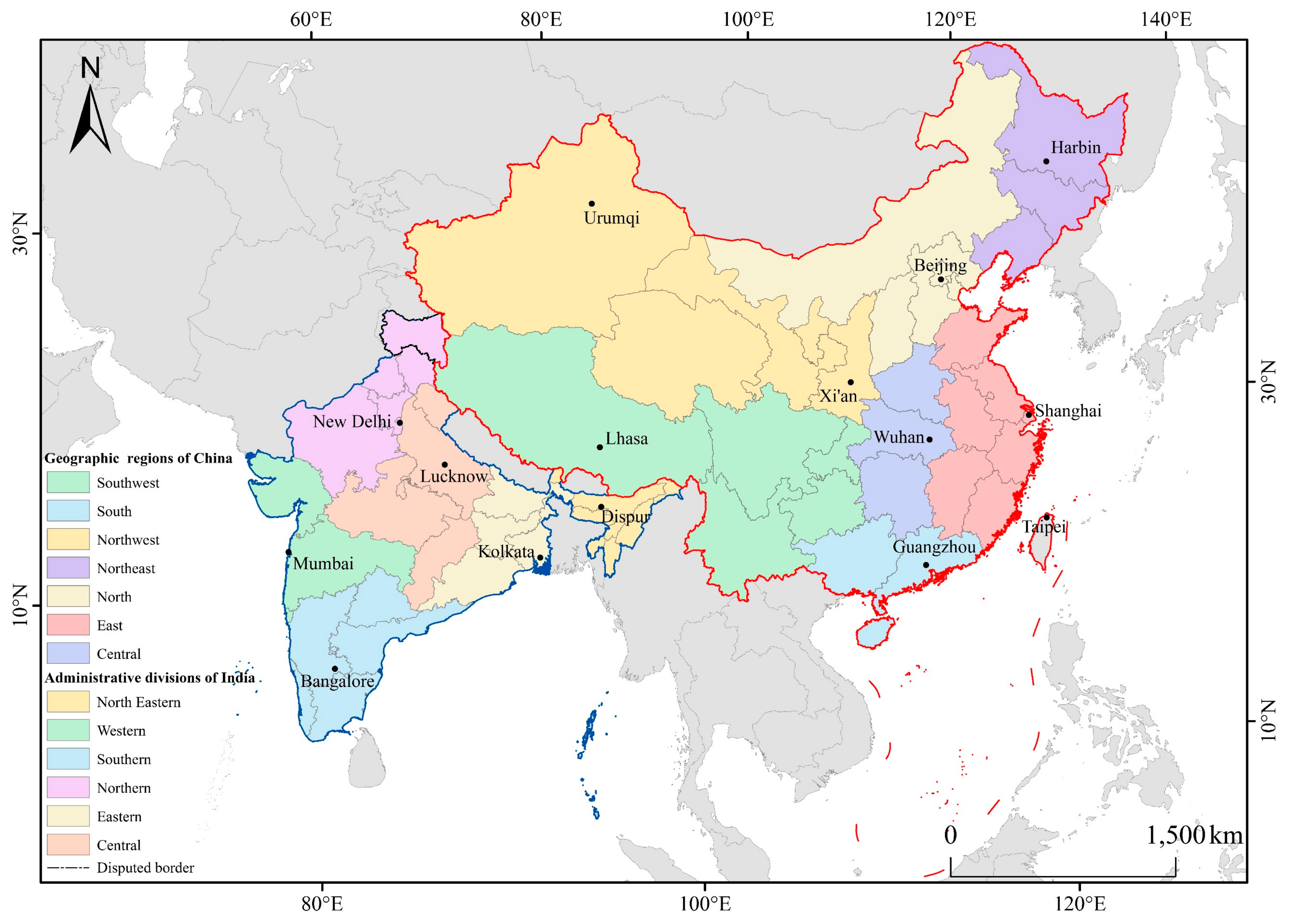
2.1. Study Area

This article takes China and India as the research areas. China is situated in the Asia-Pacific core region combining eastern Asia to the west coast of the Pacific Ocean, which ranks third in the world of a land area about 9.6 million km² and is also the most populous country in the world. India is the largest country in the South Asian subcontinent, which ranks seventh in the world in land area, with an area of 2.98 million km² about one-third of China’s land area and is the second most populous country after China. On a regional scale, China is divided into seven regions, and India is divided into six regions (Figure 1). At present, there are 35 administrative divisions in India, of which the state of Telangana was separated from Andhra Pradesh in 2014. In 2012, there were 34 first-level administrative divisions in India, including 27 states (Pradesh) and 7 union territories; 640 second-level administrative divisions, namely district units; and 3894 third-level administrative divisions, namely tehsil units, also known as towns in India. At the end of 2010, there were 34 first-level administrative divisions in China, including 23 provinces (including Taiwan), 4 municipalities, 5 autonomous regions, and 2 special administrative regions (Hong Kong and Macao). The number of second-level administrative division was 333, including prefecture-level cities, districts, and autonomous prefectures. The third-level administrative divisions include 2856 county-level units (including municipal districts and county-level cities). Different levels of administrative divisions are taken as research units in this paper (excluding Hong Kong, Macao, and Taiwan of China) to conduct an in-depth analysis of differences in regional development between China and India on a spatial scale.

2.2. Data Sourcing and Preprocessing

At present, nighttime light (NTL) remote sensing data, obtained by the US Air Force DMSP-OLS sensor in the 1970s, have the longest time series and are the most widely used [27]. The data were released by the National Environmental Satellite Data and Information Service (NESDIS) (http://ngdc.noaa.gov/eog/index.html), part of the National Oceanic and Atmospheric Administration (NOAA). DMSP-OLS was originally used to monitor nighttime cloud volume and was later found to be able to detect light emitted by towns at night [28], which led to extensive research and the application of nighttime light remote sensing. At the same time, NTL brightness index reflects the activity intensity of the urban spatial economy, which is very suitable for large-scale urban spatial expansion research. The DMSP/OLS used in this study is the fourth edition of global nighttime lighting data. Six satellites were used to collect NTL data, among which two satellites were in service at the same year (1994, 1997–2007), and a total of 34 images were collected. DMSP/OLS non-radiation-calibrated nighttime light image includes three image types: global cloudless observation frequency image data, global average light image data, and global stable light image data. Globally stable light images include long-lasting light sources in cities, towns, and other places, and have eliminated the effects of accidental noise such as moonlit clouds and oil and gas combustion from them, which is useful for analyzing light in cities and towns. The night light image has a latitude ranging from 65° S to 75° N and a longitude ranging from 180° E to 180° W, with a spatial resolution of about 1 km and a digital number (DN) ranging from 0–63. The area where the DN value is 0 is an unlit area. The larger the DN value of the cell in the image, the larger the light intensity value of the area.

Since OLS sensors mounted on different DMSP satellites do not perform on-board calibration and mutual correction of image data, the data with a long time series between different sensors in different years is not continuous and comparable. In order to minimize the inter-annual error caused by different sensors and environmental factors, it is necessary to preprocess the original night light data. In this paper, the quadratic regression model proposed by Elvidge et al. [29] is used to conduct mutual calibration of the NTL image data from 1992 to 2012. The regression model is

$$D{N}_C=C_0+C_1\times DN+C_2\times D{N}^2$$

(1)

where C₀, C₁, C₂ are regression coefficients provided in Elvidge et al. [29], DN is the original pixel value of DMSP-OLS, and DN_C is the corrected pixel value. Elvidge et al. determine that F121999 has the brightest average values, so all other nighttime light image is intercalibrated to match its range. For our choice of an invariant area for the regression, since both China and India have a wide land area as the constant target area, we followed the method of Elvidge et al. global-scale regression in using Sicily.

The mutually calibrated images are cropped to the spatial extent of China and India, re-projected onto an Albert’s equal-area projection, and resampled to 1 km. Since there are two satellites in service in some years, the stable light data of the same year were averaged as the pixel values of that year. For ease of study, the cells of DN < 3 were reclassified as 0, and the cells of the DN > 63 after intercalibration were reclassified to 63. Next, lights were summed for each region and province in China and India, generating total lights per region and province for every year from 1992 to 2012.

2.3. Methodology

2.3.1. Gini Coefficient

The Gini coefficient is a relative indicator that can generally reflect the degree of difference in the overall or partial distribution [30]. Its value ranges from 0 to 1, the value below 0.2 means ‘absolute average’, and above 0.5 means ‘disparity’. This paper uses the Gini coefficient to study the balance of light at the regional and provincial levels in China and India. An increase of the Gini coefficient corresponds to an increase in inequality, indicating the spatial imbalance of national development. Conversely, a decrease corresponds to an increase in the degree of equality, indicating that the country’s development is spatially balanced.

2.3.2. Coefficient of Variation

The coefficient of variation is used to measure the difference in regional development at different scales and described the temporal and spatial dynamics of regional development at different scales in China and India. This coefficient has been widely used in geospatial difference research [31].

$$C_v=\frac{1}{\overline{x}}\sqrt{{\displaystyle \sum _{i=1}^n{(x_i-\overline{x})}^2}/(n-1)}$$

(2)

where C_v is the coefficient of variation, n is the total number of cells corresponding to a certain scale, x_i is the average DN value of the ith unit, and $\overline{x}$ is the average of x_i.

2.3.3. Hot Spot Analysis

The Getis–Ord Gi* index is mainly used to determine the hot spots and cold spots of geographical phenomena [32]. This paper uses the Getis–Ord Gi* index to analyze the cold spots and hot spots at different scales in China and India, revealing the heterogeneity of the spatial pattern of development in China and India. The formula is

$$G_i^{*}(d)={\displaystyle \sum _{j=1}^n{W}_i{}_j{X}_j-\overline{X}{\displaystyle \sum _{j=1}^n{W}_i{}_j}}/S\sqrt{(n{\displaystyle \sum _{j=1}^n{W}_i{{}_j}^2-({\displaystyle \sum _{j=1}^n{W}_i{}_j{)}^2}})/(n-1)}$$

(3)

where X_j is the attribute value of element j; W_ij is the space weight matrix; space is adjacent to 1, space is not adjacent to 0; n is the total number of elements; $\overline{X}$ is the mean; and S is the standard deviation. From the obtained P value and Z score, it can be found that the high value or low value element spatially generates a clustering position. If the P value is significant, the Z score is positive and the value is large, indicating that the high value clustering of the region is tight. If the Z score is negative and the value is small, the low values of the region are clustered. The tighter the class, the more prominent the cold spot. If the Z score is close to zero, there is no obvious spatial clustering.

2.3.4. Urban Expansion Intensity Index

In order to compare the strength of national core city expansion in different research periods, this paper uses the urban expansion intensity index to represent the spatial distribution of urban expansion for those periods [33]. The formula is

$$UEII=\frac{\left[\left(UD{N}_{t+i}-UD{N}_t\right)\times \frac{100}{i}\right]}{SDN}$$

(4)

UEII represents the expansion strength of the urban built-up area in the spatial range between $t$ and $t+i$ years; $UD{N}_{t+i}$ and $UD{N}_t$ represent the area of the urban built-up area in $t+i$ and $t$, respectively; and $SDN$ represents the spatial extent of the total area inside.

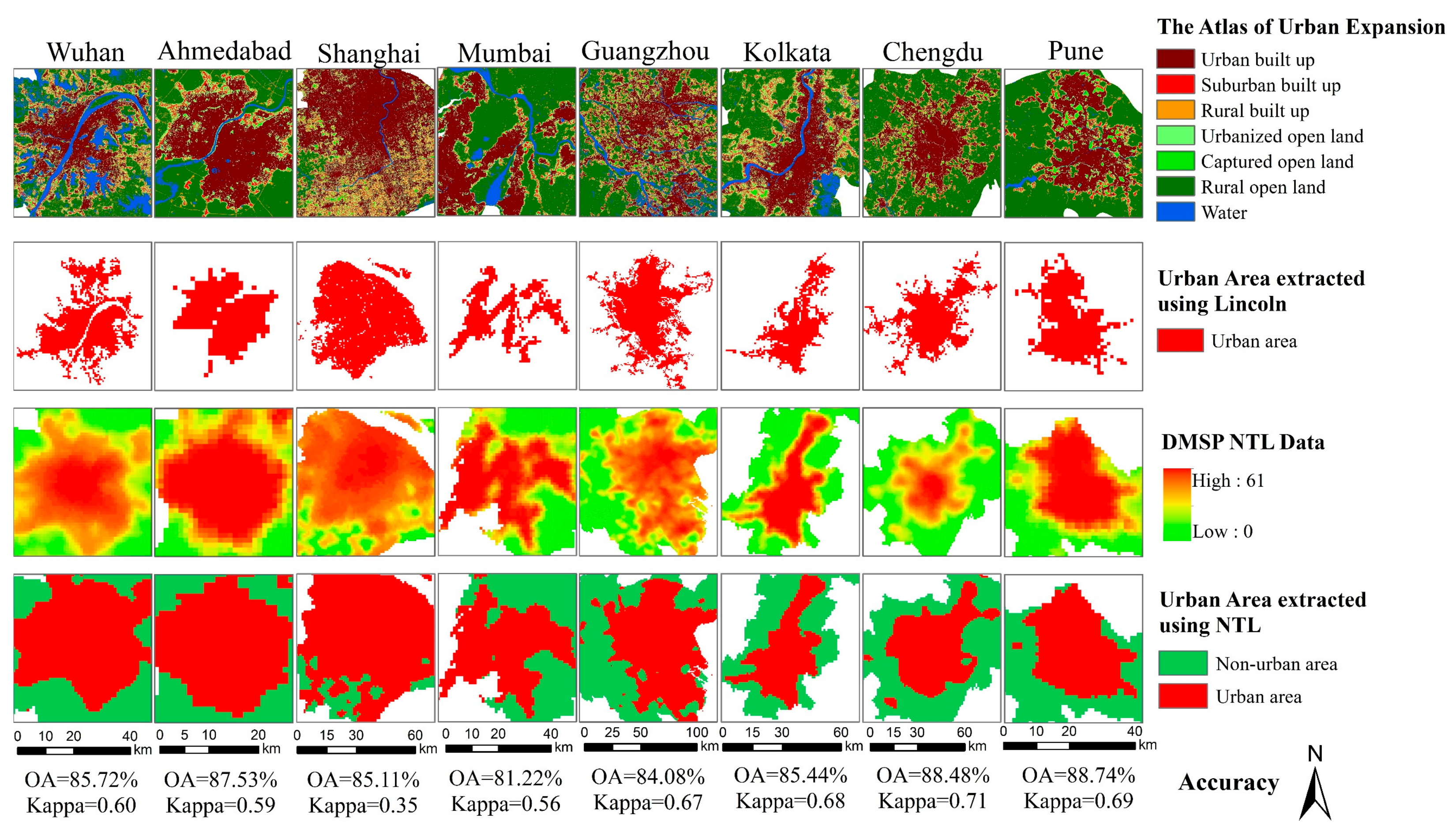
2.3.5. Extraction of Urban Built-Up Areas

Identifying the threshold of light which can represent the urban spatial range is very important for analyzing urban spatial expansion. Based on the urban spatial boundary extracted from high-resolution remote sensing image data, Henderson [34] selected core cities, such as San Francisco and Beijing, to determine the threshold of urban spatial boundary, extracted from night light data, and found that the overall precision rate of the Beijing urban area reaches 92.80% when DN exceeds 30. Ma et al. [35] divided the area of human activity into five categories using the division method of a local scale quadratic curve, and the area with a DN greater than 32 represented the suburb connected with the edge of the central city. Therefore, in order to make the urban area extracted by nighttime light data more realistic, this paper synthetically considers the best experiential segmentation threshold selected by predecessors, and on this basis, sets a dynamic threshold for each city’s light data in different years. Then the threshold is constantly changed to match the data of a reference urban built-up area, and finally, the local optimal threshold is determined for each city in different years. After determining the area of urban built-up area by the local optimal threshold, the urban expansion of the city in $i$ years was calculated as the area of urban built-up area in $t+i$ year minus the area of urban built-up area in $t$ year.

3. Results

3.1. Spatial and Temporal Evolution Characteristics of National Scale Differences

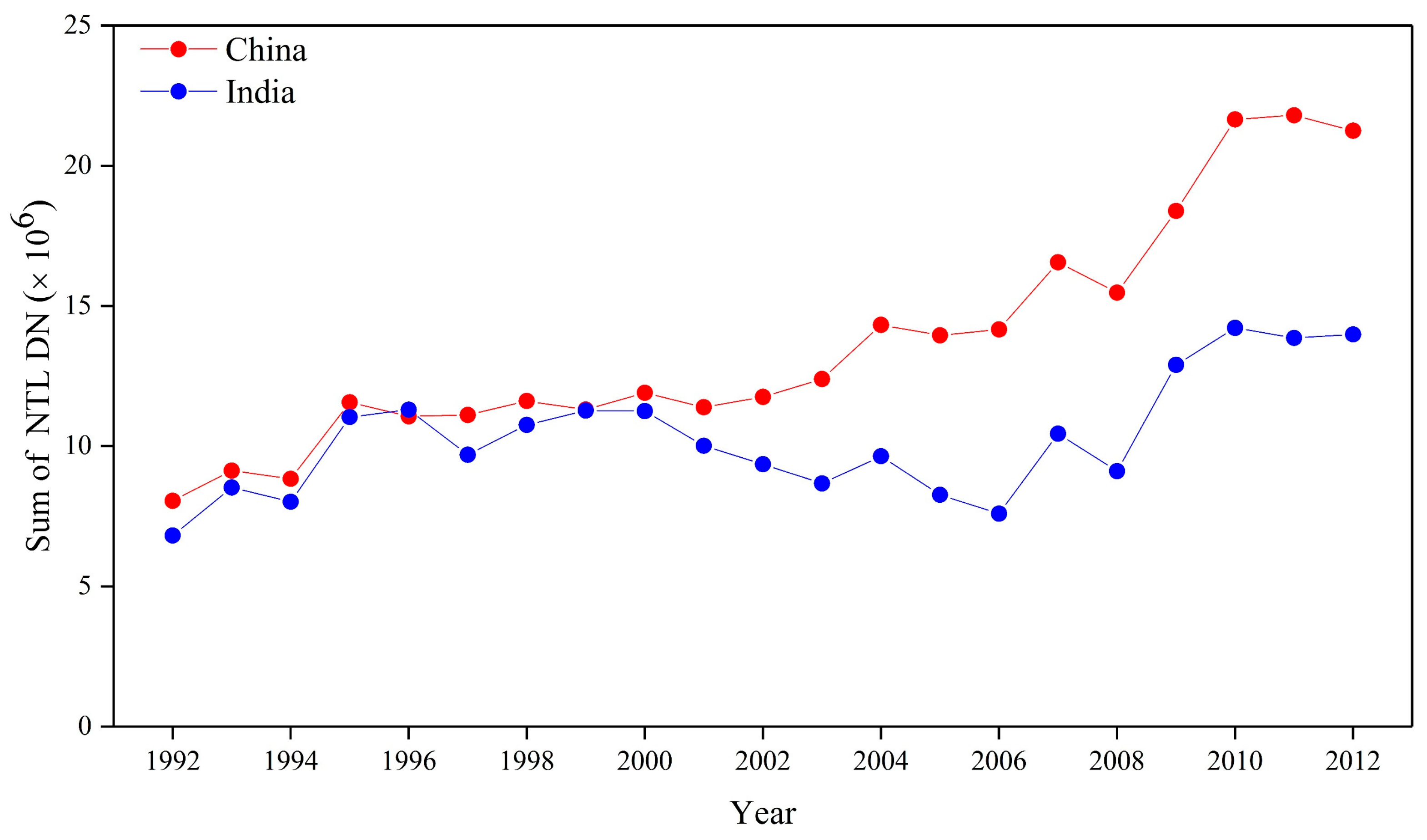
3.1.1. Temporal Evolution Characteristics

As emerging powers, China and India have similar development processes, whose total lights have a similar evolutionary trend over time. In 1992, total lights in China were slightly higher than those in India. Under the continuous influence of economic reform and globalization strategies, India began to inflow a large amount of foreign capital, and its total lights briefly surpassed China’s for the first time in 1996. In the following years, total lights in India closely followed China. However, after the accession to the WTO in 2001, China has rapidly integrated with the international community and the global economy, and the total lights in China changed greatly. As a result, the gap between the two countries is extending. India was affected by the third India-Pakistan war in 1999, during which heavy military expenditure seriously hindered India’s economic development, and India’s total lights gradually decreased from 2000 but began to develop rapidly in 2007 (Figure 2). It is worth noting that the average annual growth rates of China and India in 1992–2012 were about 5.24% and 3.85%, respectively, with China’s growth being 1.36-times that of India.

Descriptive statistics are used to calculate and analyze the changes in various types of light intensity on a national scale from 1992 to 2012. The DN values are classified according to the classification rules established by Henderson [34] combined with the light brightness values (

Table 1. Descriptive statistics for lights in China and India

Attribute	India		China
	1992	2012	1992	2012
DN = 0 (%)	70.82	49.59	91.95	82.31
DN = 4–5 (%)	19.15	26.12	3.89	5.86
DN = 6–10 (%)	5.97	15.91	2.05	6.80
DN = 11–20 (%)	2.50	5.41	1.14	2.24
DN = 21–61a/60b (%)	1.48	2.66	0.94	2.67
DN = 62a/61b (%)	0.08	0.31	0.02	0.12
Sum of all lights (DN)	6819899	13987576	8056700	21246952

^a Top-code for intercalibrated composite in 1992. ^b Top-code for intercalibrated composite in 2012.

), where DN = 0 represents “no illumination area”, DN = 4–5 and DN = 6–10 represent “dim area”, DN = 11–20 and DN = 21–62 represent “bright illumination area”, and DN = 63 represents “light saturation area”. Studies have shown that from 1992 to 2012, light in China and India both showed a trend of range extension and brightness increasing across the country. The light percentage of DN = 0 in China decreased from 92% in 1992 to 82% in 2012, while that in India decreased from 71% in 1992 to 50% in 2012, which further confirms the extensive diffusion of human beings over the earth since the early 1990s [36]. In particular, the sum of the proportions of three categories of pixel (DN = 4–5, DN = 6–10, and DN = 11–20) in India increased from 27 to 47%, along with the percentage of DN = 0 dropped from 71 to 50%, making the light distribution of India more uniform at low brightness levels. The categories of pixel values with the largest growth rate in China were DN = 21–62 and light saturation value. However, because of the dense population in southeastern China and the sparse population in northwestern China, the percentage of DN = 0 only decreased from 92 to 82%. As a result, the overall coverage of lights in India was wider than that in China, but the range of high brightness values in India was lower than in China (Figure 3).

3.1.2. Spatial Evolution Characteristics

In order to reflect the geographical significance of the spatial light variation between China and India over the past 20 years. we visualize the differences in lights between the first, middle, and final years of the 1992–2012 time period, the F101992, F152002, and F182012 composites were combined into a single three-band raster in ArcGIS 10.5. This resulted in the tritemporal map of lights for China and India. In Figure 4, 1992 values were input into the blue channel, 2002 into the green channel, and 2012 into the red channel, with the raster displayed using a standard deviation stretch (n = 2.5). In the result of composite, white indicates a stable area having a relatively constant brightness every year. Blue–purple represents a degraded area, that is, an area where the brightness is decreasing. Red represents the areas was brightest in 2012, suggesting recent growth. Green indicates the area is slow-growing in light, indicating that the lights in this region grew at the beginning of the 21st century, but that the growth rate was slow. As shown in Figure 4, the most obvious white areas in China are concentrated in the Beijing-Tianjin-Hebei, Yangtze River Delta, and Pearl River Delta urban agglomerations. The Yangtze River Delta urban agglomeration, with Shanghai as the core, is surrounded by red pixels, indicating that the cities near the Yangtze River Delta have grown more recently. The Beijing-Tianjin-Hebei urban agglomeration with Beijing as the core is surrounded by red and green pixels, indicating that the cities around Beijing-Tianjin-Hebei began to grow rapidly in the early 21st century. Although the Pearl River Delta urban agglomeration is one of the fastest growing regions in the world, it appears to be relatively white, possibly due to the limitations of DMSP-OLS sensors that cannot detect further light enhancement beyond the saturation level. In addition, the most obvious red areas in China were Hohhot and Ordos in Inner Mongolia and Urumqi in Xinjiang. Although located in the arid northwest, these newly growing cities have been able to grow rapidly because of their rich resources [37]. China’s blue–purple regions, namely recession-type regions, are concentrated in cities such as Shenyang City in Liaoning Province and Changchun City in Jilin Province, which belong to the core cities of the old industrial bases in Northeast China, but due to China’s reform and opening up policy and the southward shift of the economic center, a “Rust Belt”, similar to that of Detroit in the United States, has appeared in northeast China.

The stable development zone of light in India is concentrated in big cities such as New Delhi, Mumbai, and Bangalore. The developments on both sides of New Delhi show an obvious difference, and the west side is red–green and the east side is blue–purple, indicating that the towns on the west side grow faster while the growth of towns on the east side is gradually declining. In addition, the difference in development between northern and southern India is obvious. The southern areas are mainly green, while red and purple predominate in northern areas. In the early 21st century, the southern area began to develop rapidly while development in the northern area lagged behind. There are more green areas in Himachal Pradesh and Punjab, due to the influence of the National Rural Employment Guarantee Act (NREGA) implemented by the Indian government in the early 21st century to address unemployment and poverty [38]. It is worth noting that India’s newly growing cities are clustered in cities such as Ragar, in the north of Chhattisgarh and are growing rapidly on the basis of regional resources, while recession regions are located in cities such as Varanasi in Uttar Pradesh. Due to the large populations of these cities and the influence of traditional religions, a “Rust Belt” similar to that of Detroit in the United States has appeared.

3.2. Evolution Analyses of Regional and Provincial Scale Differences

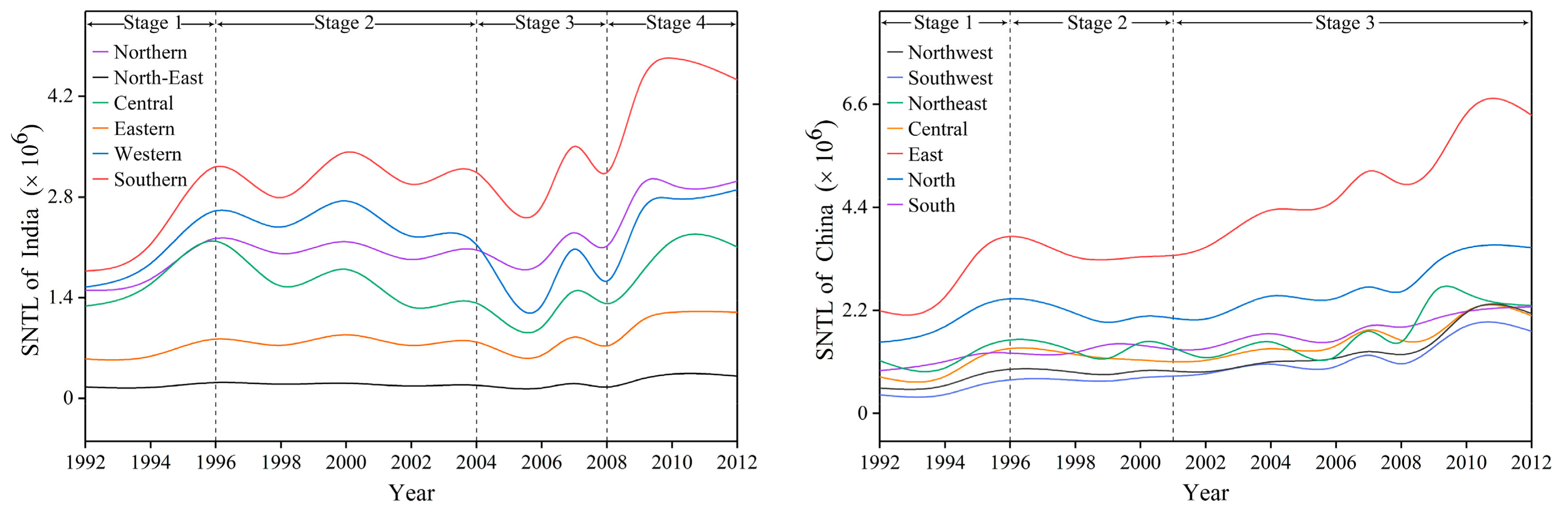
3.2.1. Regional Differential Evolution Analysis

The “World Inequality Report”, written by Thomas Piketty et al. [39], analyzed the global state of income inequality and highlighted that the degree of inequality was reduced to some extent because of the rise of China and India. Developing economies, led by China and India, have succeeded in closing the gap between poorer and more highly developed economies. The analysis of regional scale shows that the development levels of different regions of China and India shows increase tends (Figure 5). The northeastern areas in both China and India show different developing trends from other regions. Northeastern India maintains a flattening growth rate while Northeastern China shows high overall volatility. Forming an overall evolutionary trend of different regions in China and India, the development curve is divided into different stages, and it of China is divided into three stages, and India is divided into four stages. China experienced a period of rapid growth from 1992 to 1996, because China launched economic reforms under the leadership of Deng Xiaoping in 1992, and its economy maintained a sustained high growth rate. Between 1997 and 2001, China experienced a slowdown in development rate affected by the Asian financial turmoil in 1997–1998, though its economy was not directly affected due to the implementation of more cautious financial policies. The “Western Development” strategy was implemented to reduce regional inequality in 1999, and the “Rise of Central China” and “Northeast Revitalization” strategies were proposed in the following years. 2002–2012 was a sustained growth period for the development of China, and China’s accession to the WTO in 2001 and the acceleration of opening-up have brought China’s economic take-off to the forefront. China has rapidly integrated with the international community and the global economy and has gradually become the developing country that attracts the most foreign investment. Due to the impact of the subprime mortgage crisis in 2008, however, its growth rate declined. China adopted a series of protective measures to stimulate economic growth and took the lead in obviating the economic crisis, and in 2010, China became the second largest economy in the world. The development of India from 1992–2012 is divided into four stages: 1992–1996 was a period of rapid growth which witnessed the substantial positive effects of major economic reforms implemented in 1991 and have put the economy on a fast track of rapid growth during 1992 to 1996. The period from 1997 to 2004 was a stable stage because, due to the exchange crisis and the Asian financial turmoil in 1997, economic development did not improve significantly. The period between 2004 and 2008 was a stage of volatile decline. The impact of the subprime mortgage crisis in 2008 and the country’s fragile economic base forced the economic growth rate to decline rapidly. In contrast, 2009–2012 was a period of rapid growth, and India entered the top 10 economies in the world in 2010.

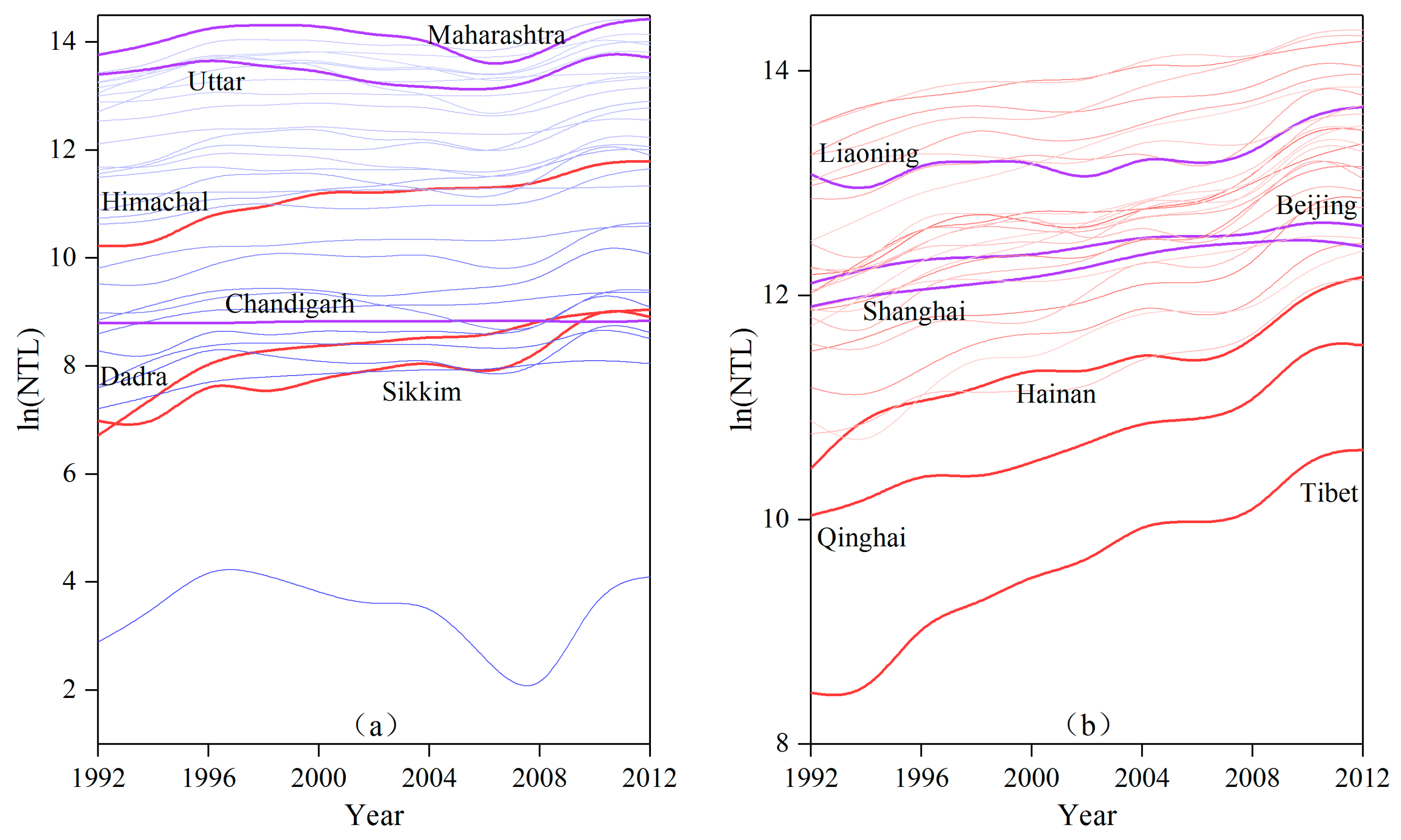
3.2.2. Provincial Differential Evolution Analysis

In order to compare the development of the lights of the provinces (states) of China and India from 1992 to 2012, the natural logarithm of the lights was used to compare the provinces with large differences (Figure 6), and the curves in the figure were smoothed to highlight the overall varying trend. The overall lights in China and India show a growing trend, the difference between them was the variation rate of light. The change of lights in most provinces in China show a high rate, while the variation rate in most states in India tends to be flat and lower than that in various provinces in China. In 1992, the provinces with lower lights in China caught up with those with higher light, and some provinces in western and northern China, such as Tibet and Qinghai, experienced the fastest rate of variation in lights. These underdeveloped northwestern provinces have grown faster than developed regions such as Beijing and Shanghai. What is noteworthy is that Hainan Province, the southernmost island-province in China, has a slower rate of variation in light compared with that of the northwestern region of China, but it also shows a rapid growth trend, which can be attributed to slow development in the past and the recent strong government support for tourism [40]. In addition, western China is also rich in energy resources, such as oil and gas. At the beginning of the 21st century, the Chinese government applied energy development as part of the regional development strategy in northwest China [41]. In India, the fastest light variation rate occurs in the states of the northeast and west such as Sikkim, Goa, and Dadra-Nagar Haveli, which are growing faster than developed states such as Chandigarh, Kerala, and Maharashtra. It is worth noting that Himachal Pradesh, a state in the northwestern part of the Himalayas, has about 90% of its population living in rural areas, and its light variation rate shows a high growth trend. Its rapid growth of lights may be attributed to many plans formulated by the Indian government to combat poverty, unemployment, and inequality. A slower increase rate of light occurred in Uttar Pradesh in northern India, where the ‘Rust Belt’ is located, and similar with conditions in Jilin and Liaoning provinces in China.

3.2.3. Regional and Provincial Difference Measures

In order to analyze the developmental differences between China and India at the regional and provincial scales, and to explore the differences in evolution law, the Gini coefficient and coefficient of variation were used. The Gini coefficient is one of the indicators in the United Nations Commission on Sustainable Development (CSD) sustainable development evaluation index system. The Gini coefficient of lights is mostly used for comparison at the national level [42,43]. Here we combine the coefficient of variation to study development status at the regional and provincial levels in China and India. (1) Regional scale: The coefficient of variation among regions in China is larger than that in India, but the Gini coefficient of China is smaller than that in India (Figure 7a). The difference in development among different regions in China shows a slight decreasing trend. Both the Gini coefficient and the C_v rise at first and then decline. The Gini coefficient increases from 0.29 in 1992 to 0.32 in 1994 and then decreases to 0.24 in 2012. The C_v increases from 0.74 in 1992 to 0.84 in 2006 and then decreases to 0.76 in 2012. The differences between the six regions in India are still relatively obvious, and the regional development differences generally increase. The Gini coefficient and C_v rise first and then decline, showing an overall increasing pattern, increasing from 0.28 and 0.44 in 1992 to 0.32 and 0.49 in 2012, respectively, reaching a maximum of 0.37 and 0.62 in 2003. (2) Provincial scale: The Gini coefficient and coefficient of variation of China are smaller than those of India, and the regional difference in India is more obvious than that in China. The evolution of differences between provinces in China shows a decreasing trend on the whole (Figure 7b). The Gini coefficient rises first and then declines, increasing from 0.44 in 1992 to 0.46 in 1994 and then decreasing to 0.38 in 2012, while C_v shows a continuous decline, decreasing from 1.71 in 1992 to 1.23 in 2012. The evolutionary trend of the differences among the state in India is similar to that in China; that is, variations in the Gini coefficient and in C_v are similar, showing a slow and general decreasing trend. India’s Gini coefficient increases from 0.64 in 1992 to 0.66 in 1999 and then falls to 0.63 in 2012, while C_v decreases from 2.16 in 1992 to 1.56 in 2012. In summary, the Gini coefficient and coefficient of variation of China and India differ in the evolution curves at different scales, and the years with the highest value are also different. The development difference between China and India is more obvious at the provincial scale than at the regional scale. This indicates that the scales have an important impact on development differences. Within the same research time series, even if the same indicators and measurement methods are adopted, the statistical results will greatly depend on the specific scale.

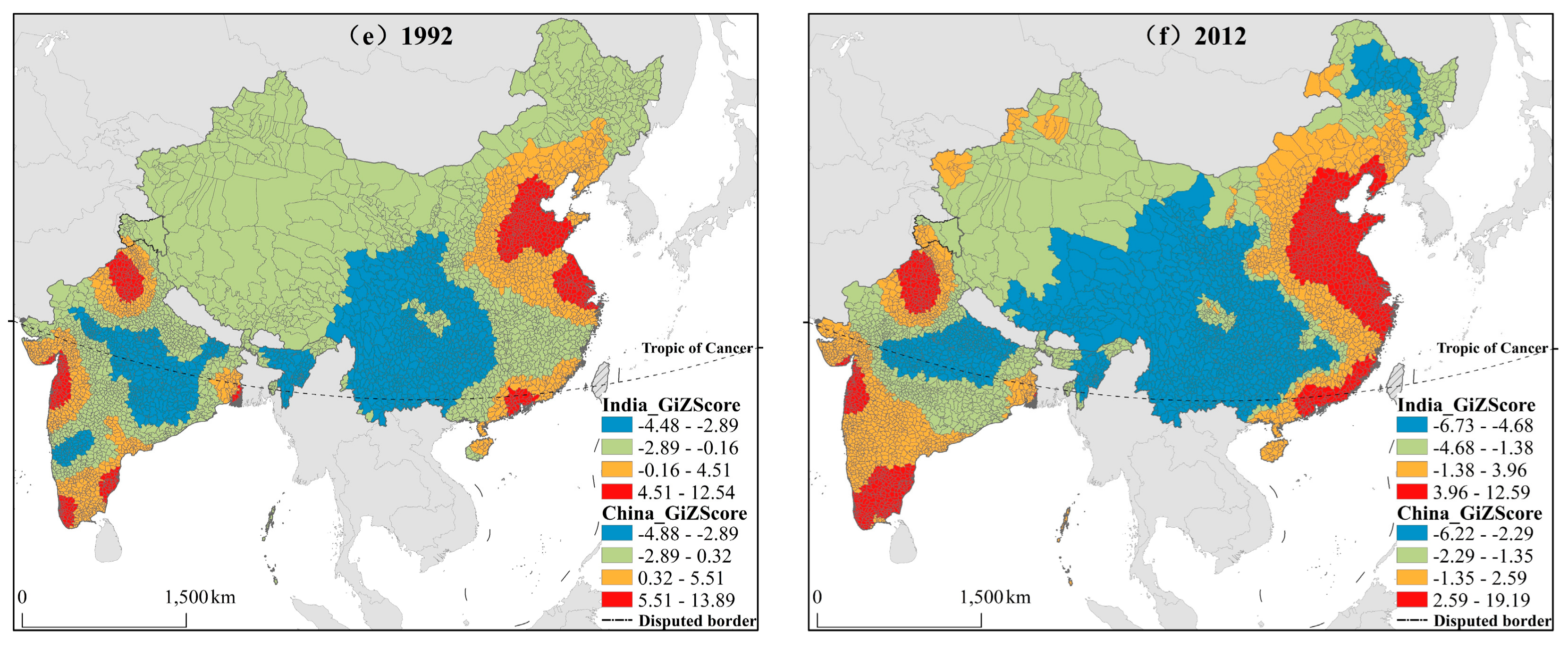
3.3. Spatial Pattern Analyses of Multi-Scale Regional Differences

Here, we further analyze spatial correlation characteristics of regional development and spatial heterogeneity characteristics at different scales and reveal the mechanisms of regional development of China and India. The Getis–Ord Gi* index is used to analyze at the provincial, prefecture, and county level scales and to express them as hierarchical symbols. First, on the provincial scale, the pattern of hot spots in China has changed little, and cold spots have clustered further, while the hot and cold spots in India are relatively stable (Figure 8a,b). India’s hot spots are always located in Punjab, Haryana, Himachal Pradesh, and New Delhi in northern India, while its cold spots are concentrated in the northeastern states of Meghalaya and Assam. The hot spots in China have evolved from Beijing-Tianjin-Hebei and Jiangsu to Beijing-Tianjin-Hebei, and Zhejiang and Jiangsu. The cold spots are further concentrated in the northwest and southwest of China. The results at the prefecture level scale show that China’s hot spots are converging, while its cold spots are shrinking from east to west (Figure 8c,d). Cold-spot distribution in India is distinct and the number of cold spots in the north is increasing. In 1992, China’s hot spots were mainly distributed in the core cities of the Beijing-Tianjin, Dalian, Jinan, Nanjing, Shanghai, and Guangzhou in southern China. In 2012, the hot spots were further distributed in the Beijing-Tianjin-Hebei, Yangtze River Delta urban agglomerations. The number of hot spots in the Yangtze River Delta region increased, and the hot spots of Jinan and Dalian evolved into sub-hot spots, while Zhengzhou City in Henan Province evolved into a new hot spot. The pattern of cold spot areas in China was relatively stable, mostly distributed in the central and western parts of the country, and the number of cold spots also gradually decreased from east to west. In 1992, India’s prefecture-level hot spots were mainly distributed in Chennai in Tamil Nadu, Pune in Maharashtra, Mumbai, Punjab, and cities near New Delhi. In 2012, hot spots further expanded on the basis of 1992, especially those near southern Tamil Nadu [44]. The distribution of cold spots in India was relatively stable, mostly distributed in central and northeastern India, and the quantitative change shows an increasing trend in the north. The results of the county level Getis–Ord Gi* values indicate that the spatial patterns and evolutionary characteristics of hot and cold spots are more detailed (Figure 8e,f). The differences between coastal and inland areas in China have become increasingly diverse, and hot spots have spread widely in the eastern coastal areas, while the number of cold spots has increased inland. India’s north–south gap have gradually widened, cold spots have been concentrated in northern India, and hot spots are widely distributed in the south and near the capital New Delhi. In 1992, China’s hot spots were distributed in most parts of the Northern China, Eastern China, and Southern China. In 2012, the hot spots spread further and were widely distributed in the eastern coastal areas, and some parts of Xinjiang evolved into sub-hot spots. The number of cold spot areas increased, spreading from southwestern China to parts of southwestern, northwestern, and northeastern China. The transition zone between cold and hot spots is also more obvious. India’s hot spots expanded further in areas such as Maharashtra, Kerala, Tamil Nadu, Punjab, and New Delhi, in which the number of hot spots near the southern state of Tamil Nadu increased most significantly, while the number of sub-hot spots was more concentrated in southern India. The cold spot area gradually shifts from the original north–south distribution to the north of India, and the distribution pattern change is obvious.

In general, China’s hot and sub-hot spots at the provincial scale are distributed in the eastern coastal areas, and the cold spots are concentrated in the inland areas [45]. The hot spots in India are concentrated in the north and the cold spots in the northeast. At the prefecture-level scale, China’s hot and sub-hot spots are concentrated in the eastern coastal areas dominated by the Beijing-Tianjin-Hebei, Yangtze River Delta, and Pearl River Delta urban agglomerations. Cold and sub-cold areas are concentrated in inland areas and gradually decrease from coastal areas to inland. The north–south distribution of India’s cold hot spots is obvious, and the hot and sub-hot spots are mostly concentrated in the south and near the capital, New Delhi. The number of cold spots in the north is increasing. At the county level, China’s hot and sub-hot spots are widely distributed in the eastern coastal areas, and the cold spots are concentrated in the inland areas and are increasing. India’s hot and sub-hot spots are concentrated in the south and in the capital New Delhi, while the cold spots are more concentrated in Northern India.

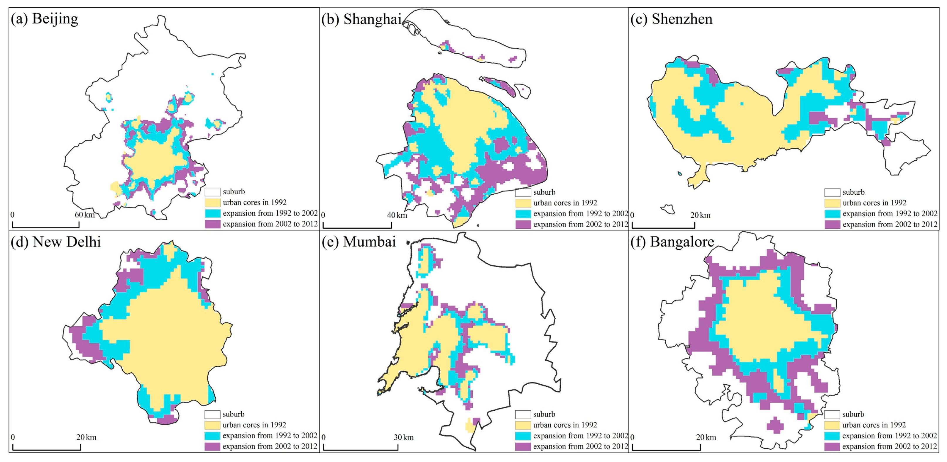
3.4. Comparative Analyses of National Core Cities

Cities are areas with a high population density and have gathered a large number of innovative resources such as capital, technology, and manpower. Core cities with different functions have important influences throughout the country in the fields of politics, economy, and science and technology, and their development level is not only related to the consolidation and promotion of the their own status but also to the overall economic and social development of the country, as well as the international competitiveness and status of the country, thus core cities are also the hot areas in geography research [46]. Urban expansion is a process of spatial outward expansion of cities, especially municipal districts and built-up areas [47]. This paper selects cities that can represent the country’s international division of labor, cooperation, and competition from the political, economic, scientific, and technological fields—such as Beijing-Delhi, Shanghai-Mumbai, and Shenzhen-Bangalore—to compare the spatial development differences between China and India. Nighttime lights data are used to simulate urban space expansion and compare urban expansion intensity.

After processing nighttime light data, a time-space expansion map of the core cities of China and India was obtained (Figure 9). Based on a comparative analysis of the core cities of the two countries in terms of an expansion mode and expansion intensity (

Table 2. Core cities’ expansion intensity index of China and India in 1992–2012.

City	1992–1997	1997–2002	2002–2007	2007–2012
Beijingp	0.2589	0.2704	0.1929	0.2561
Delhip	0.2365	0.0292	0.0053	0.4465
Shanghaie	0.5494	0.4164	0.7453	0.0882
Mumbaie	0.2433	0.0777	0.0259	0.2489
Shenzhens	0.5159	0.1720	0.2337	0.0816
Bangalores	0.3062	0.2694	0.3468	0.5756

p, e, and s represent the political, economic, and scientific centers of China and India, respectively.

), it can be found that China’s core cities are all in the multi-core expansion mode, while India is dominated by the single-core expansion mode. The expansion model of Beijing and New Delhi are quite different. Beijing has a multi-core expansion model and developed in a coordinated way with the main city as the core and a multi-sub-core in the periphery, with the expansion strength, maintained at around 0.20 and at its maximum in 1997–2002, reaching 0.27. New Delhi has a single-core expansion model. The light area based on the main city area was gradually expanded, with the expansion strength reached a maximum of 0.45 in 2007–2012, while the expansion intensity was small in 1997–2007, all below 0.05. The expansion model of Shanghai and Mumbai are similar to those of Beijing and New Delhi, respectively. Shanghai has a multi-core expansion model and its expansion intensity has remained at a high level. The expansion intensity of Shanghai reached 0.75 in 2002–2007, higher than that of the core cities of China and India in the same period. Mumbai is not only the financial capital of India, but also the world’s largest slum. From the perspective of the expansion mode of the light, Mumbai has less external expansion, and the expansion mainly based on the original foundation and the expansion strength is low, with the maximum expansion intensity being 0.24, which is at the lower level of the expansion intensity of the two countries. As the national science and technology innovation centers, the expansion modes of Shenzhen and Bangalore are dominated by the filling mode. Shenzhen centers on internal and external filling modes and is developing to the east. During 1992–1997, the expansion intensity reached the maximum value of 0.52. Bangalore was dominated by external filling modes, following an ‘urban sprawl’ model, whose expansion intensity has remained at a high level and reached 0.58 during 2007–2012, the maximum value in the core cities of China and India during the same period. In summary, the core cities of China and India have different expansion models. China’s core cities all have multi-core expansion models, while India is characterized by a single-core expansion model. During 1997–2007, China’s core urban expansion intensity remained at a relatively high level and was at a relatively low level in 2007–2012. India, however, had a lower level of expansion intensity in its core cities in 1997–2007 and had a high level in 2007–2012.

4. Discussion

Nighttime light data can more closely reflect spatial information than traditional statistical data. Therefore, the use of light data instead of statistical data to analyze the temporal and spatial dynamics of Chinese and Indian towns is more objective, simple, and has a high inter-annual comparability. However, DMSP-OLS lighting satellites still have low resolution and supersaturation problems, which affect the identification of urban growth boundaries and, hence, research accuracy to some extent. In this study, we combined the empirical thresholds and the local-optimized threshold methods to detect the core cities’ urban expansion of China and India during 1992–2012. This combined method not only identified the urban extents from both the large urban areas and small urban patches, but also effectively prevented some fragments of the suburban areas from being included in the extracted urban area for small- and medium-sized cities. In order to assess NTL-derived urban areas by this method, we compared the maps with the extracted urban areas from finer-resolution using The Atlas of Urban Expansion (TAUE) data which have been widely used to extract urban area in previous studies [48,49]. Because TAUE data has a higher resolution than NTL images (30 m vs. 1 km), it has been extensively used for assessing NTL-derived urban extents. Compared with the extracted urban areas from TAUE data, urban areas extracted using corrected NTL data well represented the spatial patterns in the study area. The average overall accuracy (OA) of urban expansion of Chinese and Indian cities in 2012 was 85.79%, and the average Kappa was 0.61. Our results are promising at the city level (Figure 10).

The urban areas extracted from TAUE data or NTL data still have many uncertainties, the main reasons for these can be categorized as: (1) the difference between impervious surfaces and NTL-based urban definitions, and (2) the oversaturation effects and coarser spatial resolution of DMSP-OLS NTL data, as well as radiation correction problems. In addition, although TAUE data are an urban area data extracted from Landsat Thematic Mapper (TM) data and proven to be feasible and acceptable, the available images still contain uncertainties due to weather effects. Meanwhile, data preprocessing inevitably leads to a loss in image fidelity. Therefore, in the future, DMSP-OLS data can be combined with a new generation of the Suomi National Polar Partnership-Visible Infrared Imaging Radiometer Suite (NPP-VIIRS) data [50] with a higher radiation resolution to improve the accuracy of town simulations. However, since nighttime lighting data from different satellites cannot be directly compared, research on strengthening data combinations should be explored in future work.

5. Conclusions

As the reform and opening-up policy enters its fourth decade, cities in China and India have developed rapidly. Based on the spatial study of night light data, it is found that the fastest growing areas in both countries are concentrated in the core cities: the Beijing-Tianjin-Hebei, Yangtze River Delta, and Pearl River Delta urban agglomerations in China; and New Delhi, Mumbai, and Bangalore in India. Cities in the resource-based regions of the two countries have developed rapidly recently, represented by Hohhot, Inner Mongolia and Urumqi, Xinjiang, in China; and Raigarh, Chhattisgarh in India.

The differences of urban development between China and India are manifested in the spatial differences in inland and coastal areas. The spatial pattern of regional development in China is mainly an east–central–west difference, while the spatial pattern of regional development in India is dominated by the north–south differences. The imbalance at the regional and provincial levels is more prominent both in China and India, and the developments imbalance among states in India is even more marked. Imbalanced development is one of the predicaments of SDGs. The Chinese government has made great achievements in reducing regional inequality. Although India has formulated a series of anti-poverty measures, the effect is not as significant as China.

References

1. Kaplinsky, R.; Messner, D. Introduction: The Impact of Asian Drivers on the Developing World. World Dev. 2008, 36, 197–209. [Google Scholar] [CrossRef] [Green Version]
2. Tripathi, S. Do Economic Reforms Promote Urbanization in India? Asia-Pac. J. Reg. Sci. 2018, 1–28. [Google Scholar] [CrossRef]
3. Wan, G. Introduction to the Special Section on “Urbanization in China”. China Econ. Rev. 2018, 49, 141–142. [Google Scholar] [CrossRef]
4. Yuan, J. The dragon and the elephant: Chinese-Indian relations in the 21st century. Washington Quarterly 2007, 30, 131–144. [Google Scholar] [CrossRef]
5. Korukonda, A.R.; Carrillo, G.; Bathala, C.; Afza, M. The Dragon and the Elephant: A Comparative Study of Financial Systems, Commerce, and Commonwealth in India and China. ICFAI J. Int. Bus. 2007, 2, 7–20. [Google Scholar]
6. Mukherjee, A.; Zhang, X. Rural Industralization in China and India: Role of Policies and Institutions. World Dev. 2007, 35, 1621–1634. [Google Scholar] [CrossRef]
7. Hölscher, J.; Marelli, E.; Signorelli, M. China and India in the global economy. Econ. Syst. 2010, 34, 212–217. [Google Scholar] [CrossRef]
8. Nigam, N. China versus India: Emerging Giants in the World Economy. In The China Business Model; Paulet, E., Rowley, C., Eds.; Chandos Publishing: Cambridge, MA, USA, 2017; pp. 215–249. [Google Scholar]
9. Kan, K.; Wang, Y. Comparing China and India: A factor accumulation perspective. J. Comp. Econ. 2013, 41, 879–894. [Google Scholar] [CrossRef]
10. Jianglin, Z. China and India: A Comparative Study of Economic Development Stage. South Asian Stud. 2011, 2, 49–68. [Google Scholar]
11. Jiaming, L.; Yu, Y.; Jie, F.; Fengjun, J.; Wenzhong, Z.; Shenghe, L.; Bojie, F. Comparative research on regional differences in urbanization and spatial evolution of urban systems between China and India. Acta Geogr. Sin. 2017, 72, 986–1000. [Google Scholar]
12. Zhang, J.; Zhou, Q.; Shen, X.; Li, Y. Cloud Detection in High-Resolution Remote Sensing Images Using Multi-features of Ground Objects. J. Geovis. Spat. Anal. 2019, 3, 14. [Google Scholar] [CrossRef]
13. Frick, A.; Tervooren, S. A Framework for the Long-term Monitoring of Urban Green Volume Based on Multi-temporal and Multi-sensoral Remote Sensing Data. J. Geovis. Spat. Anal. 2019, 3, 6. [Google Scholar] [CrossRef]
14. Nordhaus, W.; Chen, X. A sharper image? Estimates of the precision of nighttime lights as a proxy for economic statistics. J. Econ. Geogr. 2014, 15, 217–246. [Google Scholar] [CrossRef]
15. Ghosh, T.; Powell, L.R.; Elvidge, D.C.; Baugh, E.K.; Sutton, C.P.; Anderson, S. Shedding light on the global distribution of economic activity. Open Geogr. J. 2010, 3, 148–161. [Google Scholar]
16. Yi, K.; Tani, H.; Li, Q.; Zhang, J.; Guo, M.; Bao, Y.; Wang, X.; Li, J. Mapping and Evaluating the Urbanization Process in Northeast China Using DMSP/OLS Nighttime Light Data. Sensors 2014, 14, 3207–3226. [Google Scholar] [CrossRef] [PubMed] [Green Version]
17. Elvidge, C.D.; Sutton, P.C.; Ghosh, T.; Tuttle, B.T.; Baugh, K.E.; Bhaduri, B.; Bright, E. A global poverty map derived from satellite data. Comput. Geosci. 2009, 35, 1652–1660. [Google Scholar] [CrossRef]
18. Stathakis, D.; Tselios, V.; Faraslis, I. Urbanization in European regions based on night lights. Remote. Sens. Appl. Soc. Environ. 2015, 2, 26–34. [Google Scholar] [CrossRef]
19. Small, C.; Elvidge, C.D. Night on Earth: Mapping decadal changes of anthropogenic night light in Asia. Int. J. Appl. Earth Obs. Geoinf. 2013, 22, 40–52. [Google Scholar] [CrossRef] [Green Version]
20. Bennett, M.M.; Smith, L.C. Using multitemporal night-time lights data to compare regional development in Russia and China, 1992–2012. Int. J. Remote. Sens. 2017, 38, 5962–5991. [Google Scholar] [CrossRef]
21. Weipan, X.; Xun, L.; Haohui, C. A comparative research on the rank-size distribution of cities in China and the United States based on urban nighttime light data. Prog. Geogr. 2018, 37, 385–396. [Google Scholar]
22. Kuang, W.; Chi, W.; Lu, D.; Dou, Y. A comparative analysis of megacity expansions in China and the U.S.: Patterns, rates and driving forces. Landsc. Urban Plan. 2014, 132, 121–135. [Google Scholar] [CrossRef]
23. Zhou, Y.; Ma, T.; Zhou, C.; Xu, T. Nighttime Light Derived Assessment of Regional Inequality of Socioeconomic Development in China. Remote. Sens. 2015, 7, 1242–1262. [Google Scholar] [CrossRef] [Green Version]
24. Zhang, Q.; Su, S. Determinants of urban expansion and their relative importance: A comparative analysis of 30 major metropolitans in China. Habitat Int. 2016, 58, 89–107. [Google Scholar] [CrossRef]
25. Ghosh, S.; Das, A. Exploring the lateral expansion dynamics of four metropolitan cities of India using DMSP/OLS night time image. Spat. Inf. Res. 2017, 25, 779–789. [Google Scholar] [CrossRef]
26. Pandey, B.; Joshi, P.; Seto, K.C. Monitoring urbanization dynamics in India using DMSP/OLS night time lights and SPOT-VGT data. Int. J. Appl. Earth Obs. Geoinf. 2013, 23, 49–61. [Google Scholar] [CrossRef]
27. Elvidge, C.D.; Cinzano, P.; Pettit, D.R.; Arvesen, J.; Sutton, P.; Small, C.; Nemani, R.; Longcore, T.; Rich, C.; Safran, J.; et al. The Nightsat mission concept. Int. J. Remote. Sens. 2007, 28, 2645–2670. [Google Scholar] [CrossRef]
28. Croft, T.A. Nighttime Images of the Earth from Space. Sci. Am. 1978, 239, 86–98. [Google Scholar] [CrossRef]
29. Elvidge, C.D.; Hsu, F.C.; Baugh, K.E.; Ghosh, T. National trends in satellite-observed lighting. Glob. Urban Monit. Assess. Through Earth Obs. 2014, 23, 97–118. [Google Scholar]
30. Domeij, D.; Flodén, M. Inequality trends in Sweden 1978–2004. Rev. Econ. Dyn. 2010, 13, 179–208. [Google Scholar] [CrossRef]
31. Champernowne, D.G.; Cowell, F.A. Economic inequality and income distribution; Cambridge University Press: London, UK, 1998. [Google Scholar]
32. Mitchel, A. The ESRI Guide to GIS Analysis, Volume 2: Spartial Measurements and Statistics; ESRI Press: Redlands, CA, USA, 2005. [Google Scholar]
33. Zou, Y.; Peng, H.; Liu, G.; Yang, K.; Xie, Y.; Weng, Q. Monitoring Urban Clusters Expansion in the Middle Reaches of the Yangtze River, China, Using Time-Series Nighttime Light Images. Remote Sens. 2017, 9, 1007. [Google Scholar] [CrossRef]
34. Henderson, J.V.; Storeygard, A.; Weil, D.N. Measuring Economic Growth From Outer Space. Am. Econ. Rev. 2012, 102, 994–1028. [Google Scholar] [CrossRef] [PubMed]
35. Ma, T.; Zhou, Y.; Zhou, C.; Haynie, S.; Pei, T.; Xu, T. Night-time light derived estimation of spatio-temporal characteristics of urbanization dynamics using DMSP/OLS satellite data. Remote Sens. Environ. 2015, 158, 453–464. [Google Scholar] [CrossRef]
36. Geldmann, J.; Joppa, L.N.; Burgess, N.D. Mapping Change in Human Pressure Globally on Land and within Protected Areas. Conserv. Boil. 2014, 28, 1604–1616. [Google Scholar] [CrossRef] [PubMed]
37. Zhou, L.; Zhou, C.; Yang, F.; Che, L.; Wang, B.; Sun, D. Spatio-temporal evolution and the influencing factors of PM2.5 in China between 2000 and 2015. J. Geogr. Sci. 2019, 29, 253–270. [Google Scholar] [CrossRef] [Green Version]
38. Ahuja, U.R.; Tyagi, D.; Chauhan, S.; Chaudhary, K.R. Impact of MGNREGA on rural employment and migration: A study in agriculturally-backward and agriculturally-advanced districts of Haryana. Agric. Econ. Res. Rev. 2011, 24, 495–502. [Google Scholar]
39. Alvaredo, F.; Chancel, L.; Piketty, T.; Saez, E.; Zucman, G. World inequality report 2018; Belknap Press of Harvard University Press: Cambridge, MA, USA, 2018. [Google Scholar]
40. Stone, M.; Wall, G. Ecotourism and Community Development: Case Studies from Hainan, China. Environ. Manag. 2004, 33, 12–24. [Google Scholar] [CrossRef] [PubMed] [Green Version]
41. Woodworth, M.D. Disposable Ordos: The making of an energy resource frontier in western China. Geoforum 2017, 78, 133–140. [Google Scholar] [CrossRef]
42. Li, X.; Ge, L.; Chen, X. Detecting Zimbabwe’s Decadal Economic Decline Using Nighttime Light Imagery. Remote. Sens. 2013, 5, 4551–4570. [Google Scholar] [CrossRef]
43. Cauwels, P.; Pestalozzi, N.; Sornette, D. Dynamics and spatial distribution of global nighttime lights. EPJ Data Sci. 2014, 3, 2. [Google Scholar] [CrossRef] [Green Version]
44. Desmet, K.; Ghani, E.; O’Connell, S.; Rossi-Hansberg, E. The spatial development of India. J. Reg. Sci. 2015, 55, 10–30. [Google Scholar] [CrossRef]
45. Lu, Z.; Zuoquan, Z.; Wei, W. The spatial pattern of economy in coastal area of China. Econ. Geogr. 2014, 34, 14–19. [Google Scholar]
46. Liwei, W.; Chanchun, F. Spatial expansion pattern and its driving dynamics of Beijing-Tianjin-Hebei metropolitan region: Based on nighttime light data. Acta Geogr. Sin. 2016, 71, 2155–2169. [Google Scholar]
47. Angel, S.; Sheppard, S.; Civco, D.L.; Buckley, R.; Chabaeva, A.; Gitlin, L.; Kraley, A.; Parent, J.; Perlin, M. The Dynamics of Global Urban Expansion; Transport and Urban Development Department, The Wold Bank: Washington, DC, USA, 2005. [Google Scholar]
48. Xu, G.; Dong, T.; Cobbinah, P.B.; Jiao, L.; Sumari, N.S.; Chai, B.; Liu, Y. Urban expansion and form changes across African cities with a global outlook: Spatiotemporal analysis of urban land densities. J. Clean. Prod. 2019, 224, 802–810. [Google Scholar] [CrossRef]
49. Dong, T.; Jiao, L.; Xu, G.; Yang, L.; Liu, J. Towards sustainability? Analyzing changing urban form patterns in the United States, Europe, and China. Sci. Total Environ. 2019, 671, 632–643. [Google Scholar] [CrossRef] [PubMed]
50. Elvidge, C.D.; Baugh, K.E.; Zhizhin, M.; Hsu, F.C. Why VIIRS data are superior to DMSP for mapping nighttime lights. Proc. Asia-Pac. Adv. Netw. 2013, 35, 62–69. [Google Scholar] [CrossRef]
Figure 1. The location of the study area.
Sustainability 11 04509 g001
Figure 2. Annual total lights from 1992 to 2012 for China and India after intercalibration.
Sustainability 11 04509 g002
Figure 3. (a) Intercalibrated DMSP-OLS 1992 image over China and India. (b) Intercalibrated DMSP-OLS 2012 image over China and India.
Sustainability 11 04509 g003
Figure 4. Tritemporal map composite showing F10 1992, F15 2002, and F18 2012 images over China and India.
Sustainability 11 04509 g004
Figure 5. Time series of total lights plotted for each region in India and China.
Sustainability 11 04509 g005
Figure 6. Time series of total lights plotted for each province in (a) India and (b) China.
Sustainability 11 04509 g006
Figure 7. Gini coefficient and Cv at (a) regional level and at (b) province level in China and India.
Sustainability 11 04509 g007
Figure 8. Distribution of Getis–Ord Gi* values in different levels in China and India: (a,b) at the province level; (c,d) at the prefecture level; (e,f) at the county level.
Sustainability 11 04509 g008aSustainability 11 04509 g008b
Figure 9. Changes in the lighting of core cities of China and India.
Sustainability 11 04509 g009
Figure 10. Accuracy assessment of extracted urban areas from nighttime light (NTL) data through comparison with the classified maps of The Atlas of Urban Expansion in 2012.
Sustainability 11 04509 g010