A CFD Based Application of Support Vector Regression to Determine the Optimum Smooth Twist for Wind Turbine Blades


Abstract
1. Introduction
2. Methodology
2.1. Flow Solver
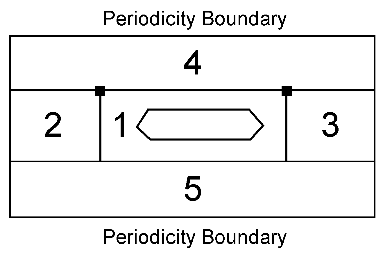
Grid Topology
- An O block around the blade
- An H block upstream the leading edge of the blade
- An H block downstream the trailing edge
- An H block up to the blade section
- An H block down to the blade section
2.2. Boundary Conditions
2.3. Unsteady Aerodynamics Experiments by the National Renewable Energy Laboratory
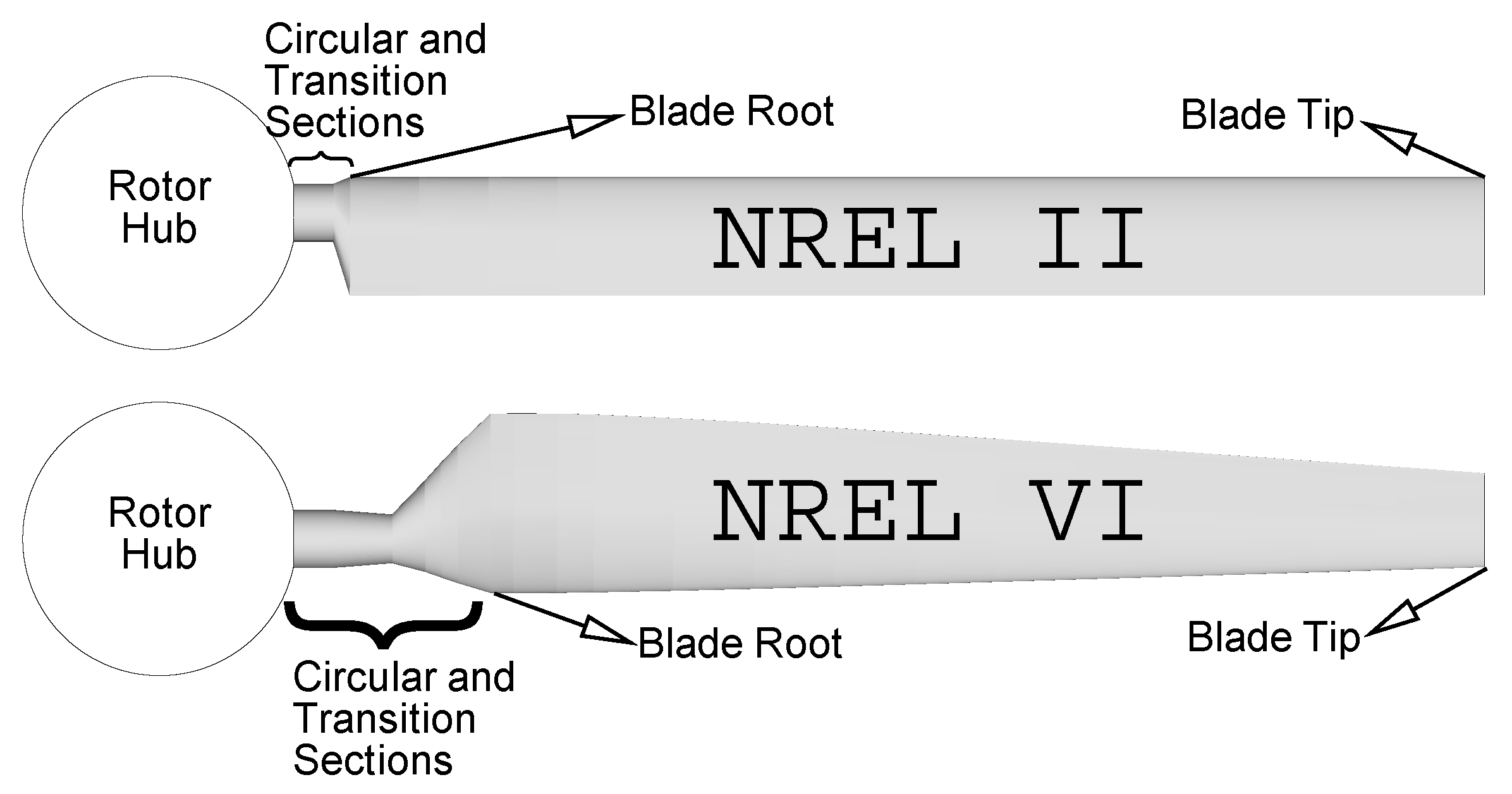
2.3.1. National Renewable Energy Laboratory II Rotor Blade
2.3.2. National Renewable Energy Laboratory VI Rotor Blade
2.4. Support Vector Regression
3. Optimization
4. Design of Experiment
- Twist angle value at the root,
- Twist angle value at the mid-span,
- Twist angle value at the tip,
- Spanwise rate of change of the twist angle at the root,
Cubic Spline-Based Twist Distribution
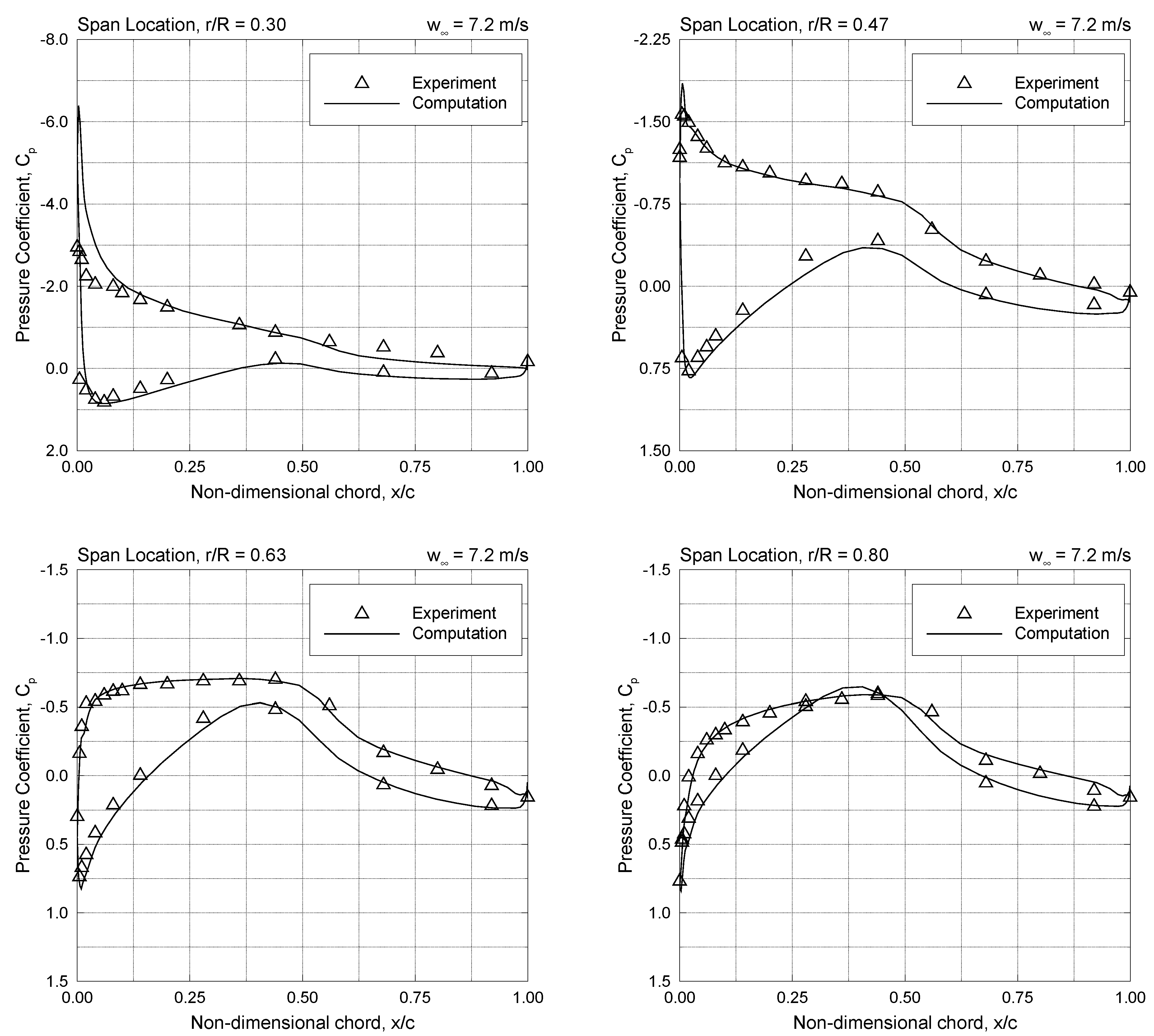
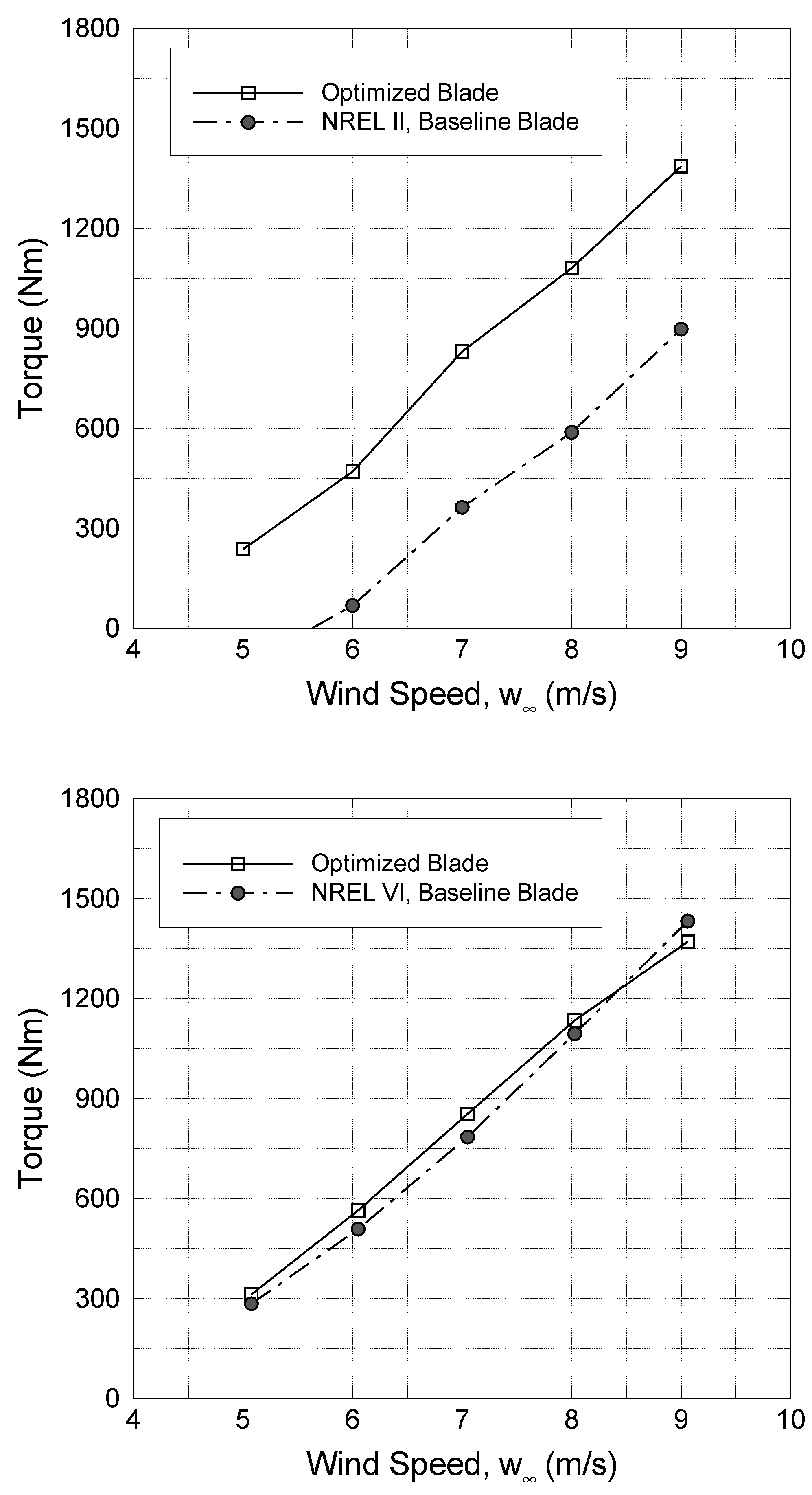
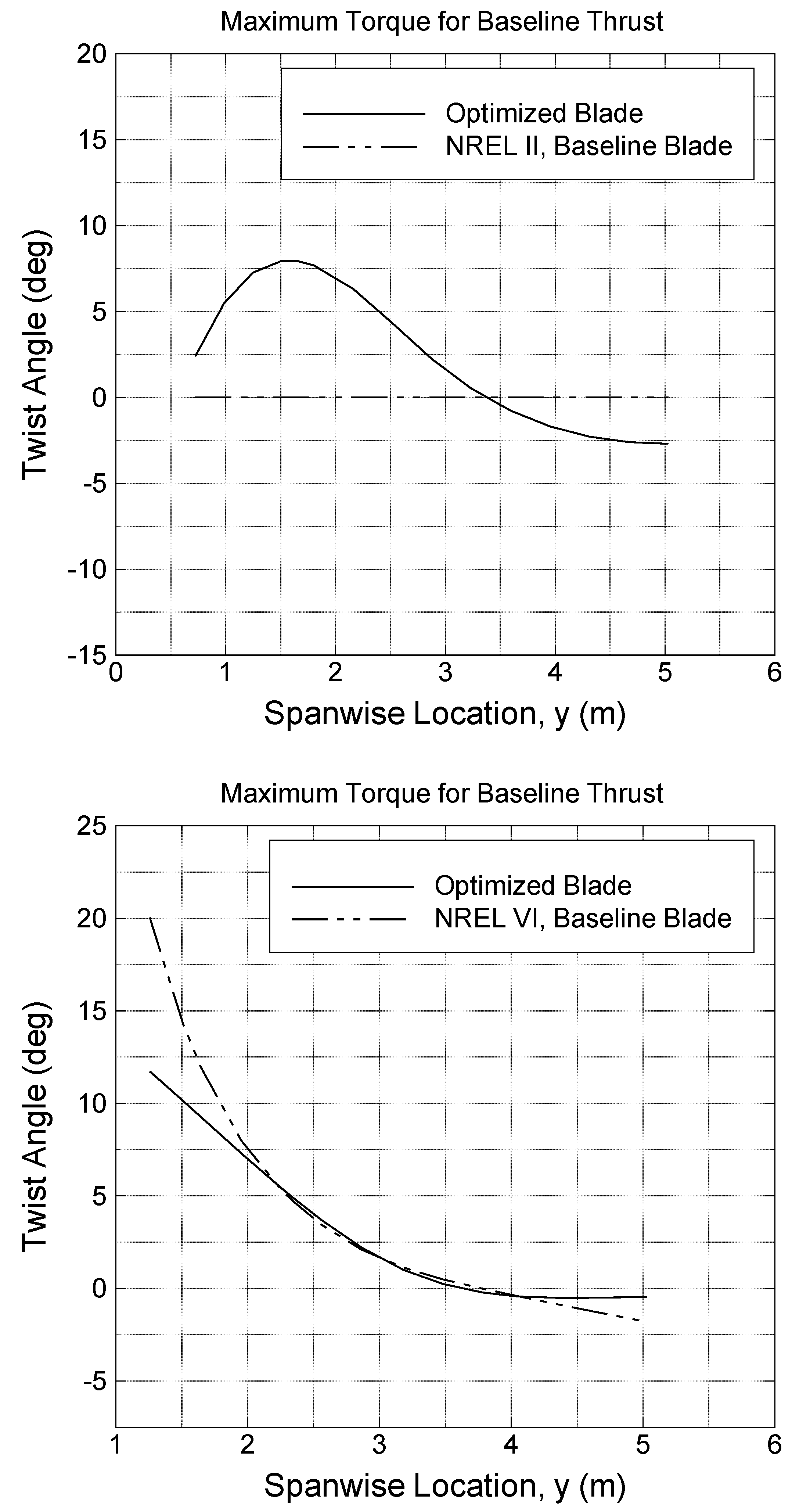
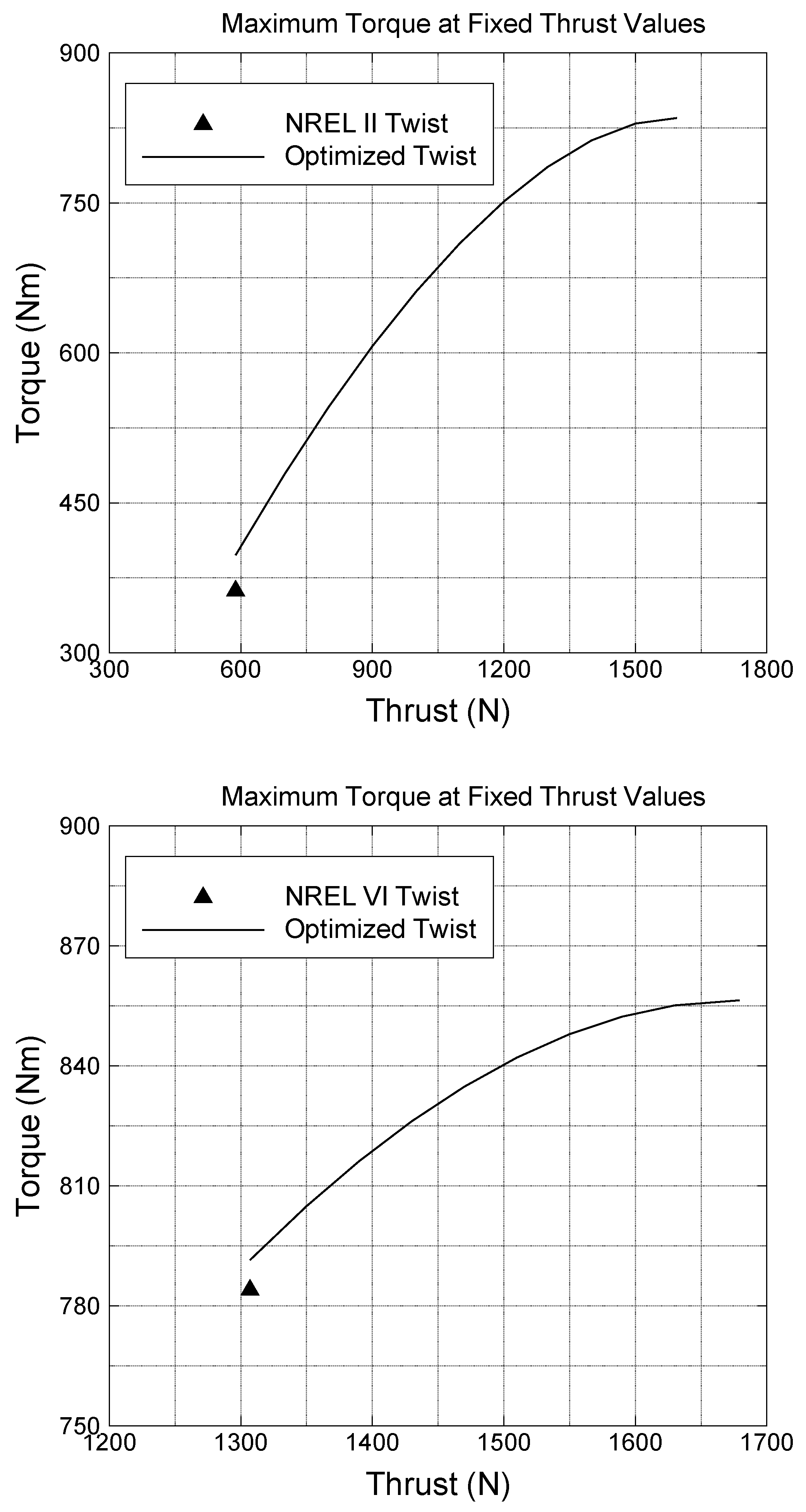
5. Validation Study
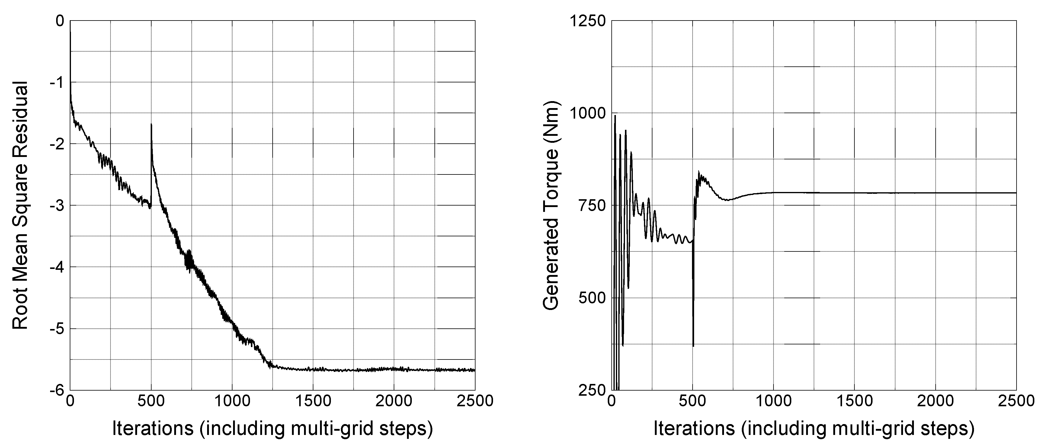
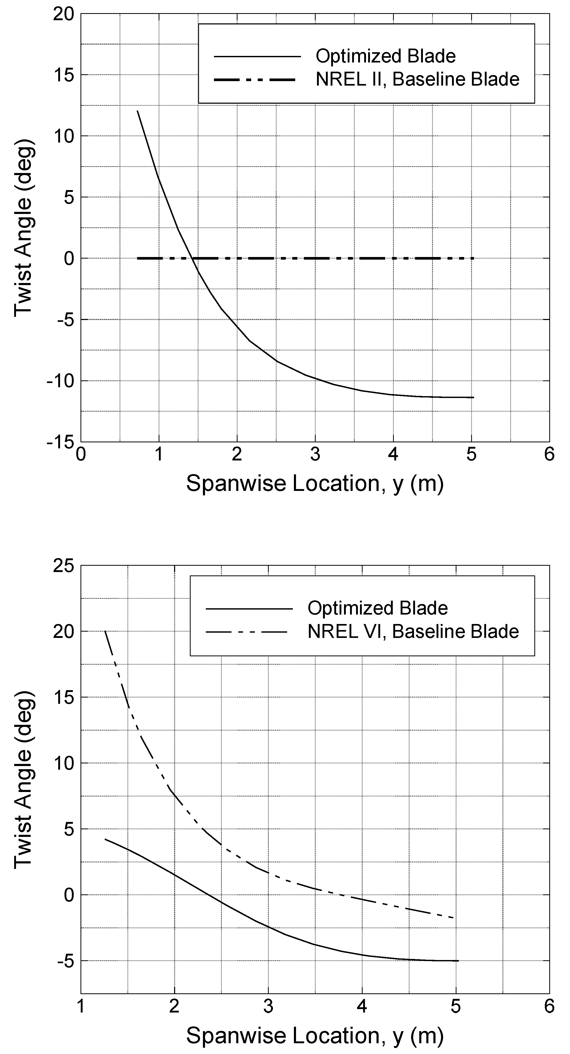
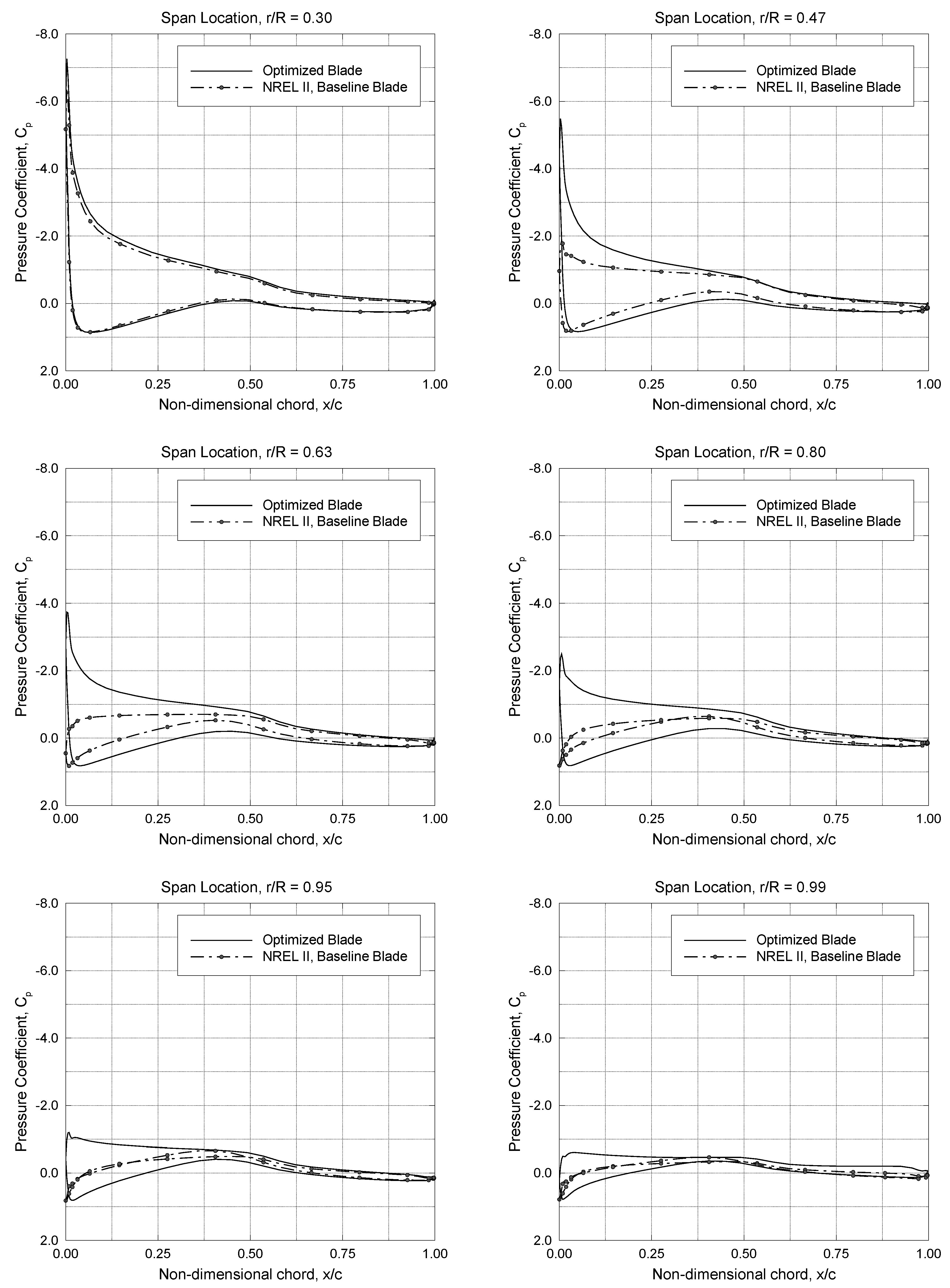
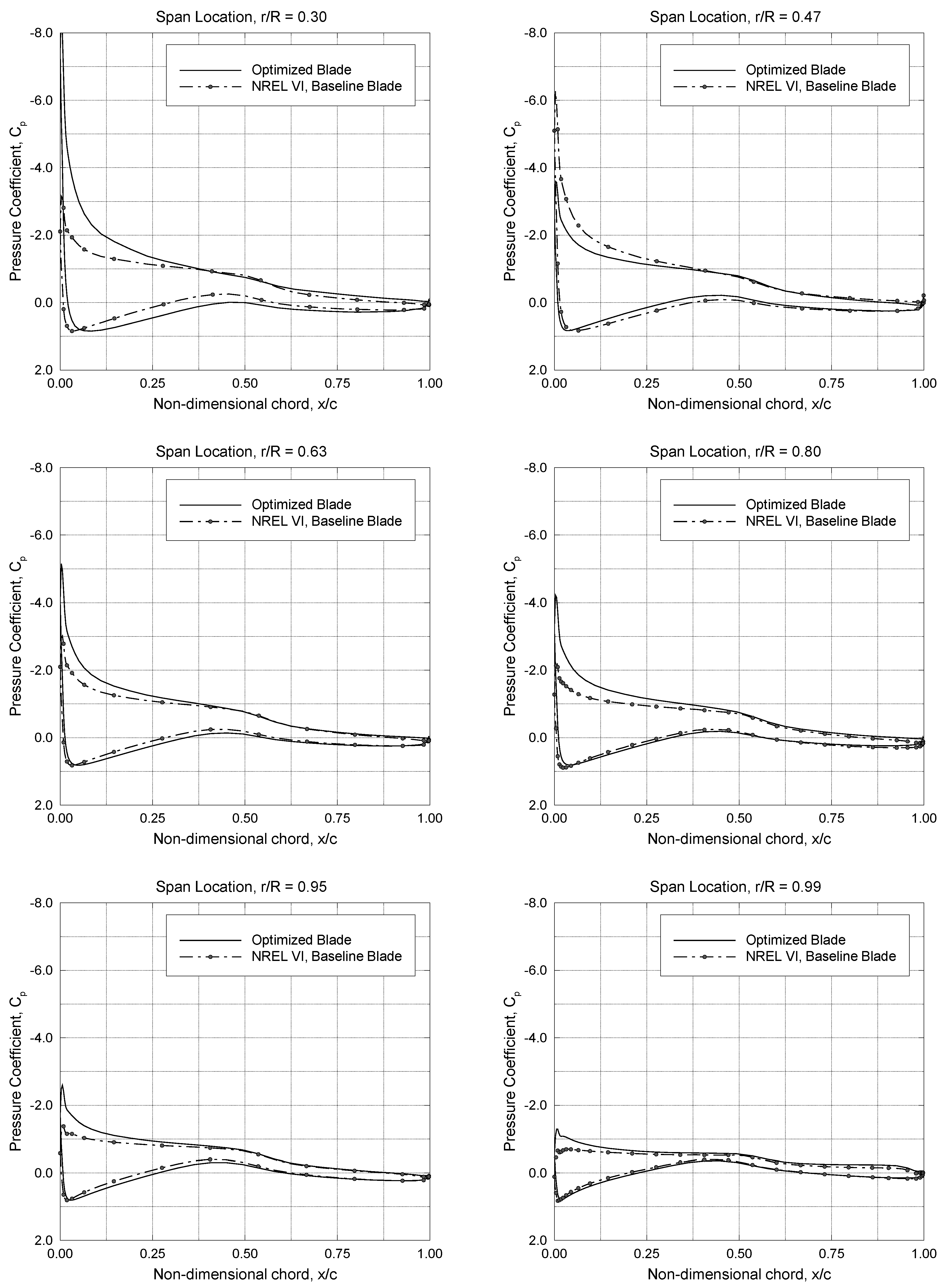
6. Results
7. Conclusions
Funding
Conflicts of Interest
References
- Iov, F.; Blaabjerg, F. Power electronics and control for wind power systems. In Proceedings of the 2009 IEEE Power Electronics and Machines in Wind Applications, Lincoln, NE, USA, 24–26 June 2009; pp. 1–16. [Google Scholar]
- Toepfer, K. Foreword: Signposts to Sustainability. In Wind Energy in the 21st Century: Economics, Policy, Technology and the Changing Electric Industry; Redlinger, R.Y., Andersen, P.D., Morthorst, P.E., Eds.; Palgrave Macmillan: Houndmills, UK, 2002. [Google Scholar]
- Salles, M.B.C.; Hameyer, K.; Cardoso, J.R.; Grilo, A.P.; Rahmann, C. Crowbar System in Doubly Fed Induction Wind Generators. Energies 2010, 3, 738–753. [Google Scholar] [CrossRef]
- Saidur, R.; Abdelaziz, E.A.; Demirbas, A.; Hossain, M.S.; Mekhilef, S. A review on biomass as a fuel for boilers. Renew. Sustain. Energy Rev. 2011, 15, 2262–2289. [Google Scholar] [CrossRef]
- Wind Technologies Market Report. Available online: https://emp.lbl.gov/sites/default/files/wtmr_final_ for_posting_8-9-19.pdf (accessed on 13 August 2019).
- Ning, A.; Damiani, R.; Moriarty, P. Objectives and constraints for wind turbine optimization. J. Sol. Energy Eng. 2014, 136, 041010. [Google Scholar] [CrossRef]
- Martins, J.R.R.A.; Lambe, A.B. Multidisciplinary design optimization: A survey of architectures. AIAA J. 2013, 51, 2049–2075. [Google Scholar] [CrossRef]
- Yu, D.O.; Kwon, O.J. Predicting wind turbine blade loads and aeroelastic response using a coupled CFD-CSD method. Renew. Energy 2014, 70, 184–196. [Google Scholar] [CrossRef]
- Imiela, M.; Wienke, F.; Rautmann, C.; Willberg, C.; Hilmer, P.; Krumme, A. Towards multidisciplinary wind turbine design using high-hidelity methods. AIAA Pap. 2015, 1462, 1–12. [Google Scholar]
- Giguere, P.; Selig, M.S.; Tangler, J.L. Blade design trade-offs using low-lift airfoils for stall-regulated HAWTs. J. Sol. Energy Eng. 1999, 121, 217–223. [Google Scholar] [CrossRef][Green Version]
- Dhert, T.; Ashuri, T.; Martins, J.R.R.A. Aerodynamic shape optimization of wind turbine blades using a Reynolds-averaged Navier–Stokes model and an adjoint method. Wind Energy 2017, 20, 909–926. [Google Scholar] [CrossRef]
- Vorspel, L.; Stoevesandt, B.; Peinke, J. Optimize rotating wind energy rotor blades using the adjoint approach. Appl. Sci. 2018, 8, 1112. [Google Scholar] [CrossRef]
- Economon, T.D.; Palacios, F.; Alonso, J.J. A viscous continuous adjoint approach for the design of rotating engineering applications. AIAA Pap. 2013, 2580, 1–19. [Google Scholar]
- Elfarra, M.A.; Sezer-Uzol, N.; Akmandor, I.S. NREL VI rotor blade: Numerical investigation and winglet design and optimization using CFD. Wind Energy 2014, 17, 605–626. [Google Scholar] [CrossRef]
- Shrestha, T.R. 3D Aerodynamic Optimization of NREL VI Wind Turbine Blade for Increased Power Output and Visualization of Flow Characteristics. Master’s Thesis, Embry-Riddle Aeronautical University, Daytona Beach, FL, USA, 2014. [Google Scholar]
- Volikas, A.; Nikas, K.-S. Turbulence modeling investigation of airfoil designed for wind turbine applications. In Proceedings of the International Conference on Technologies and Materials for Renewable Energy, Environment and Sustainability, Beirut, Lebanon, 10–12 April 2019; Salame, C.-T., Shaban, A.H., Papageorgas, P., Aillerie, M., Eds.; American Institute of Physics Inc.: New York, United States, 2019; p. 020067. [Google Scholar]
- Aksenov, A.; Ozturk, U.; Yu, P.C.; Byvaltseva, P.; Soganci, S.; Tutkun, O. A validation study using nrel phase VI experiments, Part I: Low computational resource scenario. In Proceedings of the 12th European Conference on Turbomachinery Fluid Dynamics and Thermodynamics, Stockholm, Sweden, 3–7 April 2017; KTH Royal Institute of Technology: Stockholm, Sweden, 2017. [Google Scholar]
- Rogowski, K.; Hansen, M.O.L.; Hansen, R.; Piechna, J.; Lichota, P. Detached Eddy Simulation Model for the DU-91-W2-250 Airfoil. In Proceedings of the 7th Science of Making Torque from Wind, Milan, Italy, 20–22 June 2018; Riboldi, C.E.D., Cacciola, S., Sartori, L., Croce, A., Eds.; Institute of Physics Publishing: Bristol, England, 2018; p. 022019. [Google Scholar]
- Kabir, I.F.S.A.; Ng, E.Y.K. Effect of different atmospheric boundary layers on the wake characteristics of NREL phase VI wind turbine. Renew. Energy 2019, 130, 1185–1197. [Google Scholar] [CrossRef]
- Salari, M.S.; Boushehri, B.Z.; Boroushaki, M. Aerodynamic analysis of backward swept in hawt rotor blades using CFD. Int. J. Renew. Energy Dev. 2018, 7, 241–249. [Google Scholar] [CrossRef]
- Fadl, A.; Abbasher, M.; Younis, O.; Seory, A.E. A numerical investigation of the performance of wind turbine airfoils with gurney flaps and airfoilshape alteration. J. Eng. Sci. Technol. 2017, 13, 1–16. [Google Scholar]
- Ma, Y.; Zhang, A.; Yang, L.; Hu, C.; Bai, Y. Investigation on optimization design of offshore wind turbine blades based on particle swarm optimization. Energies 2019, 12, 1972. [Google Scholar] [CrossRef]
- Chaudhary, M.K.; Prakash, S. The aerodynamic shape optimization for a small horizontal axis wind turbine blades at low Reynolds number. Int. J. Mech. Prod. Eng. Res. Dev. 2019, 8, 843–854. [Google Scholar]
- Erturk, E. Preliminary analysis of a concept wind turbine blade with piecewise constant chord and constant twist angle using BEM method. Int. J. Renew. Energy Res. 2018, 8, 4. [Google Scholar]
- Tenghiri, L.; Khalil, Y.; Abdi, F.; Bentamy, A. Optimum design of a small wind turbine blade for maximum power production. IOP Conf. Ser. Earth Environ. Sci. 2018, 161, 012008. [Google Scholar] [CrossRef]
- Tahani, M.; Maeda, T.; Babayan, N.; Mehrnia, S.; Shadmehri, M.; Li, Q.; Fahimi, R.; Masdari, M. Investigating the effect of geometrical parameters of an optimized wind turbine blade in turbulent flow. Energy Convers. Manag. 2017, 153, 71–82. [Google Scholar] [CrossRef]
- Capellaro, M.; Cheng, P.W. An iterative method to optimize the twist angle of a wind turbine rotor blade. Wind Eng. 2014, 38, 489–498. [Google Scholar] [CrossRef]
- Liu, X.; Wang, L.; Tang, X. Optimized linearization of chord and twist angle profiles for fixed-pitch fixed-speed wind turbine blades. Renew. Energy 2013, 57, 111–119. [Google Scholar] [CrossRef]
- Polat, O.; Tuncer, I.H. Aerodynamic shape optimization of wind turbine blades using a parallel genetic algorithm. Procedia Eng. 2013, 61, 28–31. [Google Scholar] [CrossRef]
- Selig, M.S.; Coverstone-Carroll, V.L. Application of a genetic algorithm to wind turbine design. J. Energy Resour. Technol. 1996, 118, 22–28. [Google Scholar] [CrossRef]
- Cao, J.; Zhu, W.; Wang, T.; Ke, S. Aerodynamic optimization of wind turbine rotor using CFD/AD method. Mod. Phys. Lett. B 2018, 32, 1840053. [Google Scholar] [CrossRef]
- Moghadassian, B.; Sharma, A. Inverse design of single- and multi-rotor horizontal axis wind turbine blades using computational fluid dynamics. J. Sol. Energy Eng. 2018, 140, 021003. [Google Scholar] [CrossRef]
- Zahle, F.; Sørensen, N.N.; McWilliam, M.K.; Barlas, A. Computational fluid dynamics-based surrogate optimization of a wind turbine blade tip extension for maximising energy production. IOP Conf. Ser. J. Phys. 2018, 1037, 042013. [Google Scholar] [CrossRef]
- Vapnik, V.; Golowich, S.; Smola, A. Support vector method for function approximation, regression estimation, and signal processing. In Neural Information Processing Systems 9; Mozer, M., Jordan, M., Petsche, T., Eds.; MIT Press: Cambridge, MA, USA, 1997; pp. 281–287. [Google Scholar]
- Mehmani, A.; Chowdhury, S.; Meinrenken, C.; Messac, A. Concurrent surrogate model selection (COSMOS): Optimizing model type, kernel function, and hyper-parameters. Struct. Multidiscip. Optim. 2018, 57, 1093–1114. [Google Scholar] [CrossRef]
- Cheng, K.; Lu, Z. Adaptive sparse polynomial chaos expansions for global sensitivity analysis based on support vector regression. Comput. Struct. 2018, 194, 86–96. [Google Scholar] [CrossRef]
- Xiang, H.; Li, Y.; Liao, H.; Li, C. An adaptive surrogate model based on support vector regression and its application to the optimization of railway wind barriers. Struct. Multidiscip. Optim. 2017, 55, 701–713. [Google Scholar] [CrossRef]
- Pal, M.; Deswal, S. Support vector regression based shear strength modelling of deep beams. Comput. Struct. 2011, 89, 1430–1439. [Google Scholar] [CrossRef]
- Pan, F.; Zhu, P.; Zhang, Y. Metamodel-based lightweight design of B-pillar with TWB structure via support vector regression. Comput. Struct. 2010, 88, 36–44. [Google Scholar] [CrossRef]
- Kromanis, R.; Kripakaran, P. Predicting thermal response of bridges using regression models derived from measurement histories. Comput. Struct. 2014, 136, 64–77. [Google Scholar] [CrossRef]
- Salcedo-Sanz, S.; Rojo-Álvarez, J.L.; Martínez-Ramón, M.; Camps-Valls, G. Support vector machines in engineering: An overview. Wiley Interdiscip. Rev. Data Min. Knowl. Discov. 2014, 4, 234–267. [Google Scholar] [CrossRef]
- Basak, D.; Pal, S.; Patranabis, D.C. Support vector regression. Neural Inf. Process. Lett. Rev. 2007, 11, 203–224. [Google Scholar]
- Clarke, S.M.; Griebsch, J.H.; Simpson, T.W. Analysis of support vector regression for approximation of complex engineering analyses. J. Mech. Des. 2005, 127, 1077–1087. [Google Scholar] [CrossRef]
- Balabin, R.M.; Lomakina, E.I. Support vector machine regression (LS-SVM)—An alternative to artificial neural networks (ANNs) for the analysis of quantum chemistry data? Phys. Chem. Chem. Phys. 2011, 13, 11710–11718. [Google Scholar] [CrossRef] [PubMed]
- Stetco, A.; Dinmohammadi, F.; Zhao, X.; Robu, V.; Flynn, D.; Barnes, M.; Keane, J.; Nenadic, G. Machine learning methods for wind turbine condition monitoring: A review. Renew. Energy 2019, 133, 620–635. [Google Scholar] [CrossRef]
- Yang, C.; Qian, Z.; Pei, Y.; Wei, L. A data-driven approach for condition monitoring of wind turbine pitch systems. Energies 2018, 11, 2142. [Google Scholar] [CrossRef]
- Saidi, L.; Ali, J.B.; Bechhoefer, E.; Benbouzid, M. Wind turbine high-speed shaft bearings health prognosis through a spectral Kurtosis-derived indices and SVR. Appl. Acoust. 2017, 120, 1–8. [Google Scholar] [CrossRef]
- Cao, L.; Qian, Z.; Zareipour, H.; Wood, D.; Mollasalehi, E.; Tian, S.; Pei, Y. Prediction of remaining useful life of wind turbine bearings under non-stationary operating conditions. Energies 2018, 11, 3318. [Google Scholar] [CrossRef]
- Pandit, R.K.; Infield, D. Comparative assessments of binned and support vector regression-based blade pitch curve of a wind turbine for the purpose of condition monitoring. Int. J. Energy Environ. Eng. 2019, 10, 181–188. [Google Scholar] [CrossRef]
- Yang, Z.; Huang, H.; Yin, Z. A fault recognition system for gearboxes of wind turbines. IOP Conf. Ser. Mater. Sci. Eng. 2017, 274, 012002. [Google Scholar] [CrossRef]
- Kusiak, A.; Li, W. The prediction and diagnosis of wind turbine faults. Renew. Energy 2011, 36, 16–23. [Google Scholar] [CrossRef]
- Shamshirband, S.; Petković, D.; Amini, A.; Anuar, N.B.; Nikolić, V.; Ćojbašić, Ž.; Kiah, M.L.M.; Gani, A. Support vector regression methodology for wind turbine reaction torque prediction with power-split hydrostatic continuous variable transmission. Energy 2014, 67, 623–630. [Google Scholar] [CrossRef]
- Erfort, G.; von Backström, T.W.; Venter, G. Numerical optimisation of a small-scale wind turbine through the use of surrogate modelling. J. Energy South. Afr. 2017, 28, 79–91. [Google Scholar] [CrossRef]
- Mohandes, M.A.; Halawani, T.O.; Rehman, S.; Hussain, A.A. Support vector machines for wind speed prediction. Renew. Energy 2004, 29, 939–947. [Google Scholar] [CrossRef]
- Schepers, J.G.; Brand, A.J.; Bruining, A.; Graham, J.M.R.; Hand, M.M.; Infield, D.G.; Madsen, H.A.; Paynter, R.J.H.; Simms, D.A. Final Report of IEA Annex XIV: Field Rotor Aerodynamics; ECN-C-97-027; Energy Research Center of the Netherlands: Petten, Netherlands, 1997. [Google Scholar]
- Simms, D.A.; Hand, M.M.; Fingersh, L.J.; Jager, D.W. Unsteady Aerodynamics Experiment Phases II–IV Test Configurations and Available Data Campaigns; NREL/TP-500-25950; National Renewable Energy Laboratory: Golden, CO, USA, 1999.
- Hand, M.M.; Simms, D.A.; Fingersh, L.J.; Jager, D.W.; Cotrell, J.R.; Schreck, S.; Larwood, S.M. Unsteady Aerodynamics Experiment Phase VI: Wind Tunnel Test Configurations and Available Data Campaigns; NREL/TP 500-29955; National Renewable Energy Laboratory: Golden, CO, USA, 2001.
- Giguère, P.; Selig, M.S. Design of a Tapered and Twisted Blade for the NREL Combined Experiment Rotor; NREL/SR-500-26173; National Renewable Energy Laboratory: Golden, CO, USA, 1999.
- FINETM/Turbo Software Package User Manual; ver.11.2rc; NUMECA International: Brussels, Belgium, 2017.
- Kody, S.; Alpman, E.; Yilmaz, B. Computational Studies of Horizontal Axis Wind Turbines Using Advanced Turbulence Models. Marmara Fen Bilim. Derg. 2015, 26, 36–46. [Google Scholar]
- Tachos, N.S.; Filios, A.E.; Margaris, D.P.; Kaldellis, J.K. A Computational Aerodynamics Simulation of the NREL Phase II Rotor. Open Mech. Eng. J. 2009, 3, 9–16. [Google Scholar] [CrossRef]
- Yan, C.; Shen, X.; Guo, F.; Zhao, S.; Zhang, L. A novel model modification method for support vector regression based on radial basis functions. Struct. Multidiscip. Optim. 2019, 60, 983–997. [Google Scholar] [CrossRef]
- Keerthi, S.S.; Shevade, S.K.; Bhattacharyya, C.; Murty, K.R.K. Improvements to Platt’s SMO algorithm for SVM classifier design. Neural Comput. 2001, 13, 637–649. [Google Scholar] [CrossRef]
- Chang, C.C.; Lin, C.J. LIBSVM: A library for support vector machines. ACM Trans. Intell. Syst. Technol. 2011, 2, 1–27. [Google Scholar] [CrossRef]
- Box, G.; Behnken, D. Some new three level designs for the study of quantitative variables. Technometrics 1960, 2, 455–475. [Google Scholar] [CrossRef]
- Elfarra, M.A. Horizontal Axis Wind Turbine Rotor Blade: Winglet And Twist Aerodynamic Design And Optimization Using CFD. Ph.D. Thesis, Middle East Technical University, Ankara, Turkey, January 2011. [Google Scholar]
- Kaya, M.; Elfarra, M. Optimization of the Taper/Twist Stacking Axis Location of NREL VI Wind Turbine Rotor Blade Using Neural Networks Based on Computational Fluid Dynamics Analyses. J. Sol. Energy Eng. 2019, 141, 011011-1–011011-14. [Google Scholar] [CrossRef]


| Parameter | Minimum Value | Intermediate Value | Maximum Value |
|---|---|---|---|
| Root twist angle in degrees, | 5.0 | 15.0 | 25.0 |
| Mid twist angle in degrees, | −2.5 | 5.0 | 12.5 |
| Tip twist angle in degrees, | −5.0 | 0.0 | 5.0 |
| Twist slope at the root in degrees per meter, | −20.0 | 0.0 | 10.0 |
| Mesh | Number of Cells | Torque (Nm) | Wall Clock Time of Computation |
|---|---|---|---|
| 1 | 754.4 | 6 min | |
| 2 | 776.4 | 12 min | |
| 3 | 781.6 | 26 min | |
| 4 | 784.0 | 35 min | |
| 5 | 784.1 | 55 min | |
| 6 | 784.4 | 78 min |
| Blade | Torque (Nm) | Increase in Torque (%) |
|---|---|---|
| Baseline NREL II | 362 | - |
| NREL II with optimum twist | 835 | 131 |
| Baseline NREL VI | 784 | - |
| NREL VI with optimum twist | 856 | 9.2 |
| Blade | Torque by SVR (Nm) | Torque by CFD (Nm) | Difference (%) |
|---|---|---|---|
| NREL II with optimum twist | 835 | 832 | 0.36 |
| NREL VI with optimum twist | 856 | 853 | 0.35 |
| Parameter | Optimized NREL II | Optimized NREL VI |
|---|---|---|
| Root twist angle in degrees, | 12.1 | 4.2 |
| Mid twist angle in degrees, | −9.6 | −2.9 |
| Tip twist angle in degrees, | −11.4 | −5.0 |
| Twist slope at the root in degrees per meter, | −22.6 | −2.9 |
| Blade | Torque (Nm) | Thrust (N) | Increase in Torque (%) |
|---|---|---|---|
| Baseline NREL II | 362 | 588 | - |
| NREL II with optimum twist | 398 | 588 | 9.9 |
| Baseline NREL VI | 784 | 1307 | - |
| NREL VI with optimum twist | 795 | 1307 | 1.4 |
© 2019 by the author. Licensee MDPI, Basel, Switzerland. This article is an open access article distributed under the terms and conditions of the Creative Commons Attribution (CC BY) license (http://creativecommons.org/licenses/by/4.0/).
Share and Cite
Kaya, M. A CFD Based Application of Support Vector Regression to Determine the Optimum Smooth Twist for Wind Turbine Blades. Sustainability 2019, 11, 4502. https://doi.org/10.3390/su11164502
Kaya M. A CFD Based Application of Support Vector Regression to Determine the Optimum Smooth Twist for Wind Turbine Blades. Sustainability. 2019; 11(16):4502. https://doi.org/10.3390/su11164502
Chicago/Turabian StyleKaya, Mustafa. 2019. "A CFD Based Application of Support Vector Regression to Determine the Optimum Smooth Twist for Wind Turbine Blades" Sustainability 11, no. 16: 4502. https://doi.org/10.3390/su11164502
APA StyleKaya, M. (2019). A CFD Based Application of Support Vector Regression to Determine the Optimum Smooth Twist for Wind Turbine Blades. Sustainability, 11(16), 4502. https://doi.org/10.3390/su11164502