Conservation Payments and Technical Efficiency of farm Households Participating in the Grain for Green Program on the Loess Plateau of China

Abstract

This study provides an empirical analysis of household technical efficiency and its determinant factors (especially conservation payments) in the context of the Grain for Green program. On the basis of a sample of 225 farm households on the Loess Plateau in 2007, we estimate household technical efficiency using the data envelopment analysis method. In addition to a traditional ordinary least square (OLS) analysis, quantile regression (QR) analysis is also deployed to explore the possible heterogeneous effects of conservation payments and other variables on the technical efficiency across the quantiles. The results suggest that when off-farm activities are taken into account, households have considerable potential for improving their technical efficiency; OLS analysis shows that conservation payments decrease household efficiency, and the QR analysis suggests that the negative impact is significant only for higher performance households; The presence of children, access of households to leased land markets, credit markets, and extension services all show heterogeneous impacts on household efficiency. On the basis of the findings of the study, policies suggestions to improve the program’s effectiveness are provided.

1. Introduction

Despite concerted efforts by governments and development-oriented Non-Governmental Organizations (NGOs), the eradication of poverty and rehabilitation of degraded environments in underdeveloped rural regions remain among the greatest challenges faced by less developed countries [1]. Subsistence farmers who depend on natural resources for food, fiber and fuel, and have reached the limits of the environment’s carrying capacity, have traditionally taken the brunt of the blame for the mutually reinforcing problems of poverty and environmental degradation [2]. In the presence of imperfect markets and institutional failures that inhibit their participation in off-farm labor markets or prevent them from investing in land-productivity-enhancing agricultural practices, small scale farmers have been obliged to make inefficient allocation choices, leading to overcultivation and overgrazing to satisfy the needs of a growing population [3,4,5]. The consequences include not only the on-site escalating land degradation and intensified poverty exacerbated by declining land fertility, but also the off-site periodic onslaughts of floods and drought with the loss of watershed functions.

Responding to the vicious circle of rural poverty and the environmental consequences of overcultivation and overgrazing, the past decade has witnessed a growing trend of policy intervention to tackle these problems with payments for ecosystem services (PES) programs such as those in Mexico, Costa Rica, and China [6]. Through this kind of program, financial incentives have been provided to those who "supply" ecosystem services, including farmers who agree to set aside sensitive land or adopt farming technologies that generate ecosystem services such as the protection of watershed functions [7]. Conservation payments contribute to increased household income directly and indirectly through the liquidity effect on participating farm households. In this way, the two objectives of environmental conservation and rural poverty alleviation are achieved in a single integrated program.

However, the payments made by conservation programs in the developing countries are generally provided by the government [8], which means they are typically made for a fixed term owing to budget constraints. Unless farm householders are able to shift their agricultural practices and other income-generating activities with the relaxation of their liquidity constraints to generate sustainable livelihoods, the programs will not succeed [5,7]. For a farmland set-aside project like the Grain for Green (GfG) program in China, the sustainability or success of the program is dependent on its ability to improve agricultural productivity or to enable households to access alternative employment opportunities [8,9,10]. Households are less likely to cultivate sloping land, which has a much lower marginal productivity of labor, if the output of the remaining farmland improves [11] or they have access to more attractive off-farm jobs [12] so that the improved income can offset the loss of agricultural output from the set-aside land.

Many previous studies have been devoted to the impact of the GfG program on participating households’ agricultural production [13,14,15,16] and their labor reallocation to more profitable activities, especially off-farm employment [7,8,9,17,18,19,20,21]. The majority of the research finds a shift of the labor force toward off-farm employment [7,12,18,19,20,21,22,23,24] which may contribute to improved household income or well-being and to sustainable livelihoods of the participating households. However, the impact on agricultural production has received less attention and the result is less clear. While some [14,18] found evidence of improved land use intensity or agricultural investments with relaxed liquidity constraint which might contribute to improved agricultural production, others show different results [13,15,21]. For example, some of the researchers [22,24] observed a decreased skilled labor supply on farm with the labor reallocated to off-farm employment, which might be detrimental to agricultural production. There is a longstanding debate about whether the relationship between on-farm and off-farm income is complementary or competitive [25,26,27,28,29,30]. Given the intricate relationship between on-farm and off-farm activities [25,26,27,28,29,30], emphasizing one aspect and neglecting the other might lead to an incomplete or misleading understanding of the program’s effectiveness, especially if off-farm employment competes with on-farm activities and leads to reduced agricultural production. However, many studies concentrating on the effect of the program on household income or household welfare are based on a simple comparison of households before and after participation, or of participants and non-participants (see Delang and Yuan [31] for a detailed review). These results might be susceptible to sample bias as a result of some unobserved heterogeneity. In addition, rising household income alone does not necessarily guarantee a sustainable or long-term livelihood [32]. Another concern is that while the conservation payments to farmers are expected to have a liquidity effect, as a kind of decoupled subsidy they may also generate a wealth effect [33]. Therefore, the impact of payments, the major measure of GfG, on the household income or welfare of farm households is unclear. Yet this potential problem has rarely been identified let alone explored explicitly in the voluminous literature on the GfG. Furthermore, the effectiveness of the program requires a more nuanced understanding of the poor households that it targets [12].

Farm household level technical efficiency is a newly developed concept [34] that is receiving increasing recognition in the empirical literature [35,36,37]. The notion of technical efficiency originates from the work of Farrell [38] and it captures the ability of the production unit to obtain the maximum possible output with a specified endowment of inputs, given existing technology and environmental conditions [39]. By extending traditional technical efficiency analysis at the farm level to the household level, this method considers the impact of farm household decisions on general household production activities, including farm production and off-farm employment. In a land set-aside program like GfG, a household level technical efficiency analysis provides important information on the performance of a household’s use of its available technology and resources, including labor, capital and the remaining farm land to maximize its household income, indicative of the sustainability of its livelihood [32]. Therefore, the objective of the present study is to estimate the technical efficiency of households participating in the GfG program and to explore the determinant factors empirically. By regressing conservation payments from the program and other factors on household technical efficiency with a traditional ordinary least square (OLS) regression analysis, this article identifies the effect of the program on sustainable livelihoods of farm households, and the constraints that prevent the optimal use of household resources and technologies for a more sustainable livelihood. In addition, a quantile regression analysis is deployed to explore the possible heterogeneous effect of the conservation payments on the technical efficiency across the quantiles (among different household groups). As the GfG program was declared to be enlarged and extended for another eight years [40], the results of this analysis will provide an empirical basis for improvements to the program policies and targeting of farm households.

The rest of the paper is organized as follows. Section 2 reviews the literature to investigate theoretically how conservation payments of the GfG program affect household technical efficiency. In Section 3, the analytical framework and the empirical models used in the paper are discussed. Section 4 discusses source and statistics of the data used in the models. The empirical results are presented and described in Section 5. The conclusions and policy implications are presented in Section 6.

2. The Grain for Green Program, Conservation Payments and Household Technical Efficiency

Triggered by the once-a-century flood along the Chang Jiang River which claimed thousands of lives in 1998, the Grain for Green (GfG) program (also known as Sloping Land Conversion Program), was introduced by the Chinese government in 1999 to tackle the serious land erosion and poverty challenges in rural China. The principal measure of the program is to “compensate farmers with grain or cash for reforesting cultivated marginal or steeply sloping lands over 25 degrees,” in order to induce land and labor reallocation to increase agricultural production and shift surplus labor to off-farm jobs [41]. The first phase of the program lasted eight years and subsequent efforts have been devoted to consolidating the achievements on formerly cultivated sloping land by reforestation and resettlement [42]. By the end of 2014, over 295 million ha of marginal or sloping lands had been reforested, affecting 32 million rural households, with an expenditure of over 405 billion Yuan (in 2014, 1 Chinese Yuan was worth 0.16 USD) [40]. Given its notable economic and environmental benefits [31], the Chinese government declared its intention in 2014 to enlarge the scale of land conversion by another 90 million ha and to compensate farmers for an additional eight years [40].

Theoretically, conservation payments affect households’ production activities (including the allocation of labor and other inputs and the adoption of new technologies) and household technical efficiency through two channels.

On the one hand, conservation payments may alleviate the liquidity constraint facing rural households and enable them to invest in more profitable farming technologies and to participate in more remunerative activities, including off-farm employment. Some empirical studies found evidence that farmers’ liquidity constraints were relaxed with the introduction of the GfG program. In such cases, agricultural practices were shifting from subsistence farming to more intensive and higher-return cash crops [7,14], with improved management practices and increased capital inputs [18]. The labor force was also shifting towards off-farm employment, such as seasonal migrant work whether formal or informal [7,12,18,19,20,21,22,23,24]. Taken individually, these changes contribute to more efficient use of labor, or capital, or land resources, or the adoption of productivity-enhancing technologies. Should all these happen together, the consequences may include increased household income and household technical efficiency. However, in developing countries where market failure is so prevalent, there is a pronounced and counter-intuitive linkage between farm and non-farm production activities [29]. Off-farm employment can boost agricultural production by further alleviating household liquidity constraints and contributing to agricultural inputs or investments [28,30], but they may also compete for household labor and capital that would otherwise be allocated to agriculture [25,43,44]. As the former is more likely to happen within a liquidity-constrained environment, the latter would be more likely when farmers face labor market failures, that is, high transaction costs in off-farm job searching, inability to find a well paid off-farm job due to information asymmetries and inadequate infrastructure, or they face high transportation or living costs in cities [26]. In the latter case, the contribution of off-farm income to household income might be compromised. Unless the contribution of off-farm income to household income outweighs the lost-labor and capital effects, off-farm employment may not contribute to increased household efficiency.

On the other hand, conservation payments resemble the characteristics of a decoupled subsidy (payments that are irrelevant to current production or prices), which may induce a wealth effect allowing farmers to work less while maintaining consumption levels [33]. Naturally, this would inhibit them from working on or off the farm. While the wealth effect has been widely tested and verified in empirical studies of decoupled subsidies [45,46,47], it is generally of less concern under the GfG program. The conspicuous exception is found in the work of Liang et al. [48], which claimed to find a negative relationship between subsidies and on-farm and off-farm income.

It is impossible to disentangle the two channels through which conservation payments affect household technical efficiency. Nevertheless, in an attempt to understand how this huge budget program fosters best use of available technologies and resources to achieve more sustainable livelihoods, it is necessary to estimate the net effect of conservation payments on household efficiency. In addition, the impact of conservation payments on different groups (quantiles), especially poorer households (or households with poor performance), has rarely been explored [12]. The quantile regression analysis provides a useful method to estimate the different effects of explanatory variables at different quantiles of the dependent variable. This would provide important information about how the program achieves its poverty alleviation goals and how the policy can be adjusted to target groups with greater precision for a more effective program.

3. Methods and Data

3.1. Household Technical Efficiency Estimation

Chavas et al. [34] has demonstrated that in the developing countries, there is jointness in the technologies underlying farm and nonfarm activities (or non-separability between farm household production and consumption decisions) due to market failures. Accordingly, they developed a method for measuring household level technical efficiency which included off-farm activities in the traditional farm efficiency estimation framework.

Following their work, we first develop a model of the household decision process. Suppose M family members in a farm household make production, consumption, and labor allocation decisions jointly for a specific time-period, and that they maximize utility U subject to budget and time constraints. Thus the household decision process can be modeled as follows:

Maximize U = U (z, l),

(1)

s.t.

• q′z ≤ p′y − r′x + N
• T_m = F_m + L_m + l_m, m = 1, 2, … M, (x, F, H, L; y, N) ∈ X,

where l denotes leisure (housework and childcare included), q′ denotes price vectors for consumption goods z, p′ denotes price vectors for farm outputs y, r′ denotes price vectors for non-labor inputs x (such as seed, fertilizer, land, etc.), N denotes off-farm income; T_m denotes the total amount of time available to the mth family member; F_m denotes the amount of time working on the farm for the mth family member, L_m denotes the amount of time working off-farm for the mth family member, l_m denotes the amount of time for leisure for the mth family member; X denotes the technology the household is facing, and (x, F, L; y, N) ∈X means outputs (y, N) can be feasibly produced with inputs (x, F, L) under technology X.

Families differ in the extent to which they are willing to substitute leisure for consumption goods, but for any given level of leisure l, nonsatiation of the utility function implies that the household will maximize its consumption, which is in turn equivalent to maximizing its profit conditional on l:

π(p, r, T − l) = Max (p′y − r′x + N),

(2)

s.t.

• F_m + L_m = T_m − l_m, m = 1, 2, … M,
• (x, F, L; y, N) ∈ X,

The profit maximization problem in Equation (2) is equivalent to the revenue maximization problem conditional on inputs (x, F, L).

τ(p, x, F, L, X) = Max_{y, N} {p′y + N: (x, F, L; y, N) ∈ X},

(3)

If a household produces as much as is feasible given its resources, the level of leisure, and the technology available, it will be technically efficient. All the efficient households constitute the production possibility frontier, and the technical efficiency of each household can be calculated according to its distance to that frontier.

Both parametric (e.g., stochastic frontier analysis) and nonparametric (e.g., data envelopment analysis, DEA) methods can be used to estimate the technical efficiency of decision-making units (DMU). DEA was employed in this study because it offers a flexible environment in which multiple inputs and outputs, even with different units of measurement, can be easily processed [49]. Both input-orientated and output-orientated models can be assumed in the DEA method to estimate the technical efficiency of DMUs. For an output-oriented model, we assume that an inefficient unit is made efficient through a proportional increase of its outputs while the inputs’ proportions are held constant; and for an input-oriented model, we assume that an inefficient unit is made efficient through a proportional reduction of its inputs while its outputs’ proportions remain unchanged. Following Chavas et al. [34], we employ the output-oriented DEA model to be consistent with the model of the household decision process. Here we should note, however, that the input-oriented efficiency under the consumption of constant returns to scale (CRSTE) scores are equivalent to the output-oriented CRSTE scores. The second stage regression analysis with input-oriented TE as dependent variable yields similar results with that using output-oriented TE as the dependent variable.

The output-oriented technical efficiency index assuming constant returns to scale (CRSTE), for the household j involved in both farm and off-farm activities that is characterized by utilization of inputs (x, F, L) in producing outputs (y, N), is given by solving the linear programming problem:

$$TE\left(x^j,F^j,L^j,y^j,N^j;X\right)={\min }_{\theta ,\lambda }\left\{\theta \right\},$$

(4)

s.t.

• $y\raisebox{1ex}{$j$}\!\left/ \!\raisebox{-1ex}{$\theta $}\right.\le {\displaystyle \sum _{i=1}^n}{\lambda }_i{y}^i$; $N\raisebox{1ex}{$j$}\!\left/ \!\raisebox{-1ex}{$\theta $}\right.\le {\displaystyle \sum _{i=1}^n}{\lambda }_i{N}^i$; ${{\displaystyle x}}^j\ge {\displaystyle \sum _{i=1}^n}{\lambda }_i{x}^i$; $F^j\ge {\displaystyle \sum _{i=1}^n}{\lambda }_i{F}^i$; $L^j\ge {\displaystyle \sum _{i=1}^n}{\lambda }_i{L}^i$; ${\lambda }_i\ge 0$.

By adding the ${\displaystyle \sum _{i=1}^n{\lambda }_i}=1$ constraint, we get the technical efficiency under the variable returns to scale assumption (VRSTE). The difference between CRSTE and VRSTE is due to scale inefficiency. Therefore, the definition of scale efficiency (SE) is given as the ratio of CRSTE to VRSTE and measures the extent to which the household is approaching the technologically optimal scale (or most productive scale size, MPSS).

3.2. Empirical Model

Empirically, we employ a two-stage procedure that involves the estimation of farm household technical efficiency scores in the first stage and regression to relate efficiency scores to explanatory factors in the second [49]. Traditionally, efficiency scores generated from the DEA method are regressed against explanatory variables using a Tobit model in the second stage [35,49]. However, the appropriateness of the Tobit model in the second stage is now a matter of debate. Simar and Wilson [50] argued that efficiency scores generated from the DEA method are serially correlated and they proposed a seven-step double bootstrapping procedure to produce consistent estimates in the second stage. Banker and Natarajan [51], on the other hand, demonstrated that a two-stage approach comprising a DEA model followed by an OLS (or maximum likelihood estimation) model yields consistent estimators when data are generated by a monotonically increasing and concave production function (as is the presumed by most production functions) separable from a parametric function of the contextual variables. Other researchers deem DEA scores as simply a statistical or theoretical measure of distance to an observed “best practice frontier” [52,53], which should not be deemed censored but fractional, and they advocate OLS instead of censor regression models like Tobit to obtain a consistent estimator. Given that both methods have a sizable following and considering the computational complexity of the Simar and Wilson approach, we opt for OLS in our efficiency regression model, to provide a consistent and simpler method of parameter estimation. Beyond the standard OLS regression model, which yields the mean effect of each independent variable on household technical efficiency, we also employ a quantile regression model to explore the heterogeneous effects of variables (market, farm or household characteristics) that are possible across the household technical efficiency distribution [54].

4. Sampling and Data

4.1. Sampling

We collected the data jointly with the Institute of Soil and Water Conservation of the Chinese Academy of Sciences. The Loess Plateau has suffered from the most serious soil erosion and poverty in China [55]. Villages in five catchments from Shaanxi Province were chosen as the study area for a survey in 2008 designed to get data for 2007. Both counties were among the pilot and demonstration areas of the GfG program, and integrated management at the catchment scale has been provided since late 1999. Local program offices were established to supervise and assist with the specific measures to be implemented in the counties, which makes the impact analysis of the program less biased. All five catchments have similar natural, economic and social conditions, and the same agronomic practices. The catchments include Zhifanggou, Xiannangou and Danangou from Ansai County, and Guoqigou and Liyongbian from Yanchang County. For the 28 villages in the five catchments, approximately 20% of the households (one-census-family household without additional persons) were selected randomly from the permanent residents of each village, in order to reach an effective sample size. Information was collected through face-to-face interviews on demographics, household income, land, labor and other input usage, asset holdings, details of participation in the program, agricultural production and off-farm employment of the farm households.

Eight observations were dropped because of data inconsistencies or unreliability, yielding usable data from 225 households. Participating farmers were offered a total of 160 Yuan (or grain of equivalent value) per mu (= 0.67 ha) of sloping land over 25° to plant trees instead of cultivation. Afforestation (establishment of trees on land that has been without forest cover for a long time) was divided into ecological forests, subsidized for eight years, and economic forests, subsidized for five years. The program was implemented jointly by local government at the county level. Agricultural extension services such as greenhouse crop management, fruit growing, and livestock breeding were provided by local farm extension agencies. Off-farm labor markets were established and easier access to loans was provided through the Agricultural Bank of China, especially for horticultural producers.

4.2. Inputs and Outputs for Household Efficiency Estimation and Explanatory Variables

The estimation of household-level technical efficiency involves the following data: two outputs including farm income and off-farm income, in thousands of Yuan; four inputs including farm labor and off-farm labor, both measured in worker-months; land, measured as the total cultivated land area in mu, both owned and rented less the land rented out (here we assume that the owned and rented cultivated land have similar soil fertility); and capital and other inputs, measured in thousands of Yuan, where capital refers to the estimated value of machinery and buildings net of depreciation and maintenance costs and other inputs, which include the total expenditures on seed, fertilizer, fodder, fuel, pesticide, irrigation, wages, and rent.

Apart from conservation payments from the GfG program, farm characteristics, household characteristics, and market characteristics affect household production decisions and thus farm household efficiency [35,46,56,57,58]. We incorporated the following variables in our second-stage regression model. Conservation_payments in thousands of Yuan are measured as an eight-year average from 1999 to 2007, to reflect the impact of government conservation payments on household efficiency. Extension_services was included as a dummy variable to capture the impact of extension services on rural household efficiency: 1 if extension visits were provided by the agents and 0 otherwise. Credit, measured as the ratio of the sum of loans obtained in the past eight years as a proportion of total household assets, is included to reflect the impact of access to credit on household efficiency. Access to credit relaxes farm liquidity constraints and facilitates more efficient inputs and technology utilization which should improve overall household efficiency. We also include Tenancy, which measures the proportion of land rented-in relative to the total area of land under cultivation. We assume that access to leased farmland helps farmers to allocate resources more efficiently thus improving overall household efficiency.

To account for the endowment of human capital, we include the Education and Child variables. The Education variable is included to reflect the influence of educational attainment of households on both off-farm employment and on farm labor productivity. Education is measured as the proportion of household members who have completed secondary level education. Child is a dummy variable, having a value of 1 if there are any children under 15 in the family, and 0 otherwise. A household’s total time available for farm and off-farm activities would be reduced if there were children in the family, and child-care also inhibits off-farm employment, thus the variable is expected to decrease the household’s technical efficiency.

To account for the endowment of land resources, we included Land/labor, which is measured as the total land area in mu owned by the household divided by the total labor force (number of adults) within the household. We assume that farms less endowed with land have a higher incentive to work off-farm and thus higher household efficiency.

Here, we need to reinforce that many previous studies have been interested in the impact of off-farm employment (or its income) on farm efficiency. However, as our study focused on household level technical efficiency, which accounts for both farm and off-farm activities, it may induce the problem of endogeneity if we include it as an explanatory variable. Therefore, we checked the difference in mean efficiency estimates for off-farm participating and non-participating households instead.

4.3. Descriptive Statistics of the Data

Table 1. Descriptive statistics of variables used for household efficiency estimation and econometric models (n = 225).

Variables		Mean	SD	Min	Max
Outputs	Farm Income	6.068	11.479	0.119	72.760
	Off-farm Income	9.246	7.795	0.000	48.800
Inputs	Land	8.585	4.966	0.800	30.000
	Farm Labor	1.407	0.633	0.400	4.000
	Off-farm Labor	0.931	0.583	0.000	3.000
	Capital and Other Inputs	0.840	1.290	0.033	12.340
Explanatory Variables *	Conservation_payments	3.905	3.221	0.640	37.180
	Tenancy	0.030	0.146	0.000	1.000
	Credit	0.038	0.276	0.000	3.884
	Extension_services	0.160	0.363	0.000	1.000
	Education	0.287	0.376	0.000	1.000
	Child	0.210	0.407	0.000	1.000
	Land/labor	4.296	2.813	0.267	15.000

Note: * Multicollinearity amongst the explanatory variables was checked before conducting the regression analysis.

presents descriptive statistics of the input and output variables included in the DEA model to estimate household technical efficiencies and the variables in the empirical analysis that are expected to affect household technical efficiencies.

The average labor force within a household was 2.34 persons, with 60.3% of their working time allocated to farm work (1.41 persons on average), and 39.7% allocated to off-farm work (0.93 persons on average). However, the proportion of farm income to household income (excluding government conservation payments) was only 39.5% (6.07 thousand Yuan on average), while off-farm income amounted to 60.5% (9.25 thousand Yuan on average). This suggests a much higher return to off-farm work than on-farm work. Government conservation payments to rural households amounted to 3.90 thousand Yuan on average, a large proportion of total household income. In contrast, few of the households had access to rented farmland (only 3.0% of total farmland was rented in), extension services (16.0% of all farm households), or credit (average 4.0% of total assets). The land endowment seems adequate with cultivated land of 4.3 mu per capita (compared with the average of around 1.5 mu per capita nationwide), 21% of the households had children, and the average educational level for the householders was low, only 30% of household members had completed secondary education. We should note that substantial variance exists in the sample households.

5. Results

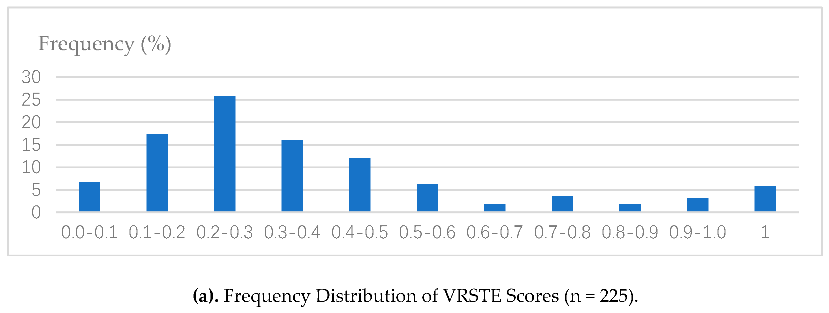
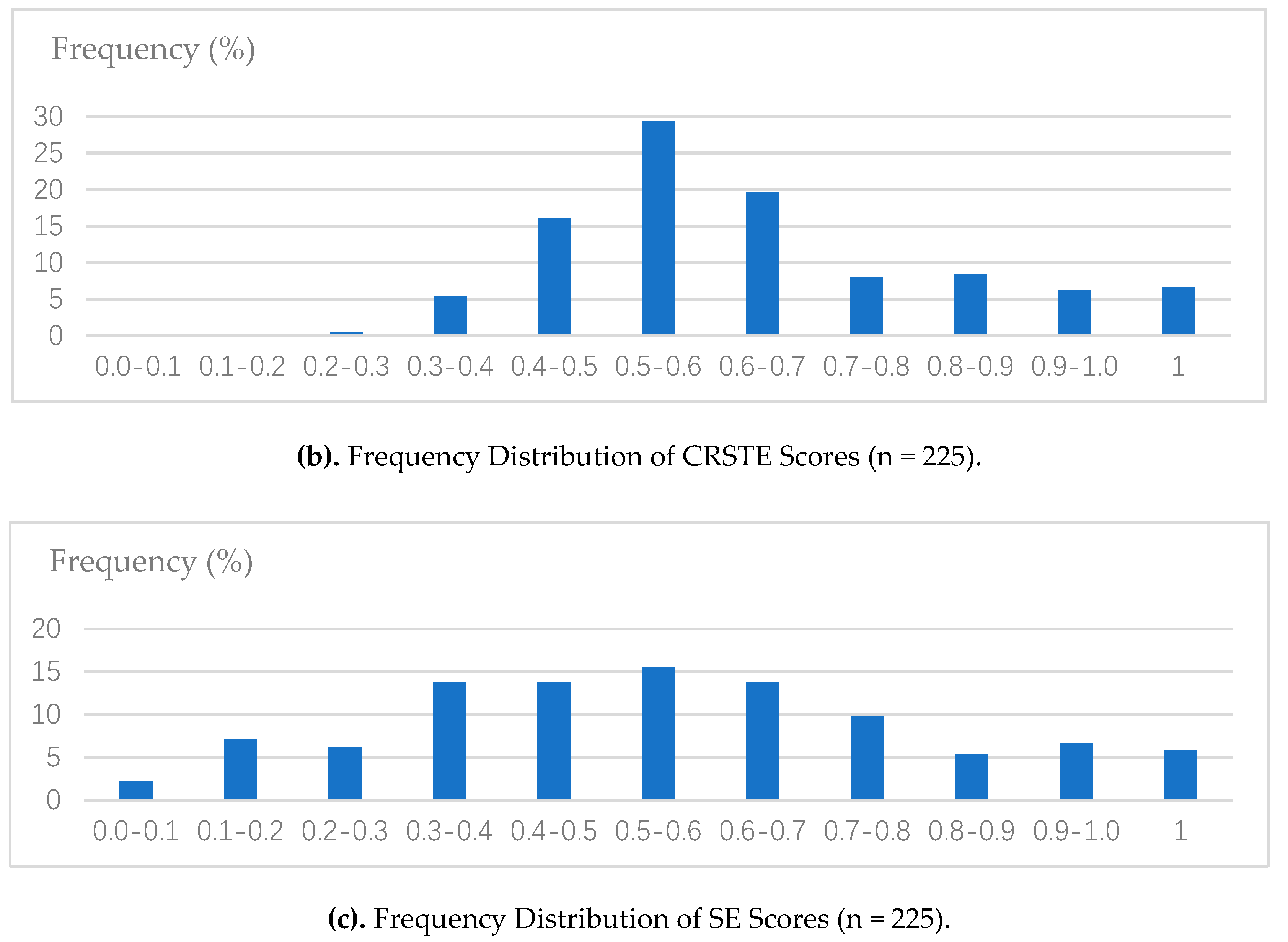
5.1. Result of Household Technical Efficiency Estimation

Technical efficiencies of the farm households under both the constant returns to scale assumption (CRSTE) and variable returns to scale assumption (VRSTE) with an output-orientation model were estimated applying DEA-Solver Pro 5.0. Descriptive statistics and frequency distributions of the efficiency scores at the household level are presented in

Table 2. Descriptive Statistics of Efficiency Scores and the Nature of Returns to Scale of Sample Households (n = 225).

Item	CRSTE	VRSTE	SE
Mean	0.382	0.669	0.555
SD	0.253	0.209	0.250
Min	0.034	0.299	0.097
Max	1.000	1.000	1.000
IRS (%)	192 (85.3)
DRS (%)	20 (8.9)
MPSS (%)	13 (5.8)

Note: CRSTE, technical efficiency under the constant returns to scale assumption; VRSTE, technical efficiency under the variable returns to scale assumption; SE, scale efficiency; IRS, increasing returns to scale; DRS, decreasing returns to scale; MPSS, most productive scale size.

and Figure 1.

The mean VRSTE of the sample households is 0.669, which means the farm households could decrease their inputs by 33.1% and still generate the same amount of farm and off-farm income. The result is quite close to another study covering a similar sample and a slightly more recent time-period, which generates a VRSTE of 0.664 at the farm level including only agricultural production activities [59]. This suggests that management skills are consistent across farm and off-farm activities. And here we should note that substantial variation exists in technical efficiencies for the sample households (SD of 0.209). The distribution shows that 176 (78.2%) of households had technical efficiency scores greater than 0.5, and 15 (6.7%) of them had a VRSTE of 1.0 (technical efficient).

We also checked the status of scale efficiency and the nature of returns to scale of households. By definition, when CRSTE is equal to VRSTE, it is scale efficient; otherwise it is scale inefficient with either increasing returns to scale or decreasing returns to scale [51]. By definition, increasing (decreasing) returns to scale indicate a situation in which an increase in output is proportionally greater (less) than a simultaneous and equal percentage change in the use of all inputs. By adding a constraint of ${\displaystyle \sum _{i=1}^n{\lambda }_i}\le 1$ to the CRSTE model, we get technical efficiency under non-increasing returns to scale (NIRSTE), and by comparing the result with that of VRSTE, we can judge whether it is operating in the area of increasing returns to scale or decreasing returns to scale. When VRSTE and NIRSTE are equal, decreasing returns to scale exists otherwise increasing returns to scale applies. In cases when NIRSTE, CRSTE and VRSTE are all equal to 1, the farm has attained the most productive scale size (MPSS). Table 2 shows that the average scale efficiency for the households was 0.555, indicating the main source of technical inefficiency for the sample households was due mainly to inappropriate production scale. Only 13 (5.8%) of sample households are scale efficient, or they were operating under the most productive scale size. The remainder (212 or 94.2%) of them were scale inefficient, mostly under increasing returns to scale (192, or 85.3%). The finding of increasing returns to scales is consistent with previous studies including only farm activities [60]. For these households, operating scales were “too small” and expanding their land, labor and capital resources proportionally would lead to a proportionally larger household income.

As mentioned in Section 4.2, we are also interested in whether there are significant differences in mean efficiency between those households that participated in off-farm activities and those that did not. We thus give an independent sample t-test on the efficiency estimates for these two subgroups (

Table 3. Difference in mean efficiency estimates between off-farm participating and non-participating households.

Efficiency Measures	Off-Farm Participants	Off-Farm Nonparticipants	Mean Difference (t-Test)
CRSTE	0.365	0.537	−0.172 ***
VRSTE	0.649	0.852	−0.203 ***
SE	0.546	0.635	−0.889

Note: *** significant at the 1% level (p < 0.01).

). Contrary to our intuition, the result suggests significantly lower technical efficiency (both CRSTE and VRSTE) for off-farm participating households compared with non-participants. In other words, off-farm employment seems to have an adverse effect on household technical efficiency, when both farm and off-farm activities were taken into account. With reference to previous literatures comparing the efficiency of these two groups of households [61,62], it may indicate that off-farm employment adversely affects farm production, or that the farmers lack the information, skills or knowledge to generate more off-farm income. And, the former might come as a result of the competitive effect of off-farm employment on labor and capital with the existence of market imperfections [25,43,44], as discussed in Section 2.

5.2. Determinants of Farm Household Technical Efficiency

The results of the regression analysis of the explanatory variables on household technical efficiencies (VRSTE) generated from the STATA software are reported in

Table 4. Ordinary least square (OLS) and quantile regression analysis of the explanatory variables on household technical efficiencies (n = 225).

	OLS Regression	Quantile Regression
	(1) VRSTE	(2) Q40	(3) Q60	(4) Q80	(5) Wald Test(p)
Constant	1.365 *** (0.181)	1.004 *** (0.342)	1.164 *** (0.302)	1.552 *** (0.332)	0.008
Conservation_payments	−0.190 ** (0.051)	−0.119 (0.093)	−0.137 * (0.082)	−0.178 * (0.096)	0.046
Tenancy	0.265 * (0.113)	0.315 (0.454)	0.193 (0.342)	0.103 (0.243)	0.368
Credit	0.068 * (0.048)	0.094 (0.050)	0.775 ** (0.421)	0.385 ** (0.259)	0.158
Extension_services	0.017 (0.045)	0.081 * (0.067)	0.098 (0.064)	0.139 (0.092)	0.021
Education	0.003 (0.037)	0.062 (0.057)	0.064 * (0.055)	0.071* (0.075)	0.574
Child	−0.131 *** (0.032)	−0.083 ** (0.042)	−0.108 ** (0.044)	−0.168 ** (0.071)	0.059
Land/labor	−0.003 (0.005)	−0.003 (0.113)	−0.005 (0.009)	−0.009 (0.008)	0.156
Pseudo R2	0.143	0.088	0.122	0.140

Note: The corresponding standard errors are reported in parentheses under parameter estimates. * Significant at the 10% level (p < 0.1); ** significant at the 5% level (p < 0.05); *** significant at the 1% level (p < 0.01).

, with OLS regression results in column 1, sequential quantile regression estimates for the 0.40, 0.60, and 0.80 quantiles of the farm household technical efficiency score distribution, and tests for equality of coefficients across quantiles, in columns 2, 3, 4 and 5, respectively. The quantile regression analysis results were generated using the Stata sqreg command.

According to the results of the OLS regression, the conservation payments to the households (Conservation_payments, significant at the 5% level) and presence of children in the family (Child, significant at the 1% level) were negatively related to household technical efficiency, while the access to credit (Credit, significant at the 10% level) and land rental market (Tenancy, significant at the 10% level) were positively related to household technical efficiency.

The negative relationship between Conservation_payments and household efficiency, might indicate that the combined result of the wealth effect of conservation payments (or compensational subsidies) and the lost labor and capital effect of off-farm employment outweigh the possible liquidity effect of the conservation payments. The wealth effect discourages farmers from exerting more effort into their production activities than would be the case in the absence of subsidies [30]. In contrast, the competitive effect of off-farm employment on labor and capital outweighs its possible positive contribution to household income and efficiency as a result of labor market failures, for example, high transaction cost of off-farm job searching, or inability to find a well paid off-farm job [27,29].

Child-care consumes total family time at home. (in our study it is not possible to separate the time spent on farming with that on housework and child-care). Families with children are more likely to face off-farm employment constraints because of the high costs of urban living and schooling, and all these constraints affect their optimal time allocation [48,63]. This might account for the negative relationship between Child and household technical efficiency.

Both the Tenancy and Credit variables are positively related to household technical efficiency. This result suggests that access to the market for rented farmland makes it possible to optimize farm area or to better allocate resources thus improving household technical efficiency. Improving access to credit may also help farm households to apply more efficient production equipment, adopt improved fertilizers or insecticides, facilitate off-farm participation, and better allocate resources thus improving productive efficiency at the household scale. This finding accords with farm level studies of small-holders in China [43,64].

The results from the quantile regression in the remaining columns of Table 3 reveal that the independent variables have different impacts on household efficiency across the whole distribution of the efficiency scores. For example, the negative impact of Conservation_payments on household technical efficiency is not significant at the 40th quantile but becomes significant at the right tail of the distribution at the 60th and 80th quantiles. One interpretation is that the conservation payments might have a larger liquidity effect on those households with poor performance or those in poverty. The quantile regression also points to a more nuanced effect of Extension_services for households in the lower part of the efficiency distribution than was revealed by the statistically insignificant OLS estimate. This suggests that providing extension services, including technical guidance and assistance is especially efficacious for lower-performing households. OLS suggests a negative relationship between Child and household technical efficiency. The quantile regression analysis shows that the impact is significant across the quantile distribution and gets stronger and stronger towards the right tail which suggests that greater attention should be directed to this issue.

6. Conclusions and Suggestions

The principal object of the GfG program is to induce land and labor reallocation towards a more sustainable livelihood with conservation payments from the government. Whether this works out, however, depends largely on the ability of the farmers to utilize the available resources (land, labor, and capital) and technologies to generate more household income, which can be measured as household technical efficiency. The aim of this study was to estimate household technical efficiency and examine the determinant factors for farm households participating in the GfG program on the Loess Plateau. We are especially interested in the impact of conservation payments on household efficiency, and we address the possible heterogeneous effect of the independent variables on households’ technical efficiency with a quantile regression in addition to a traditional OLS analysis.

The results of the empirical study suggest that farm household technical efficiency and scale efficiency under variable returns to scale averages 0.669 and 0.555, respectively, which suggest ample room exists to make more efficient use of the resources and technologies and to achieve optimal scale. The majority of households show increasing returns to scale, which suggests that expanding their operating scales would improve their scale efficiency. Households participating in off-farm activities show significantly lower technical efficiency than non-participating households, which might suggest that off-farm employment has a negative impact on farm production, or that farmers lack the information, or skills required to work off-farm. Regression analysis shows a negative impact of conservation payments on household efficiency, which may also come as a result of the competitive effect of off-farm employment (as facilitated by the program) on labor and capital, and/or the wealth effect. While the negative impact of conservation payment is especially significant for higher performance households, it is insignificant for lower performance households. The presence of children in the household might also inhibit household members’ efforts in farm and off-farm activities thus decreasing household efficiency, and the negative impact worsens for the higher quantiles. Household access to leased land and credit markets, however, seems to prompt farm households to allocate resources more efficiently, improve productivity-enhancing investments and technologies, thus improving household technical efficiency. Providing extension services also benefits those households with lower performance.

Certain limitations of this study should be kept in mind. First, as discussed in Section 3.2, we chose the OLS method, following the method used in several widely cited articles [51,52,53], to simplify the estimation and focus on a comparison of the results from OLS and from QS. However, the two-stage, double bootstrap data envelopment analysis is getting greater recognition as a means to obtain a consistent result [50,65]. The conditional efficiency approach developed by Daraio and Simar [66], which accounted for environmental variables in the efficiency estimation and which is less vulnerable to outliers and measurement error than DEA, is also increasingly advocated [67]. Future possible extensions include utilizing the double bootstrapped method to account for sampling noise and analyze the robustness of the study’s findings, or applying the conditional efficiency estimation method, especially using an order m estimator, to eliminate the possible influence of anomalous observations. Secondly, we must also acknowledge the possible limitations of our data. It was collected during the first stage of the GfG program. However, the overall design of the program has not systematically changed, and conservation payments to participating households still serve as its most important measure. While our study stresses the important role of government to remedy market failures by eliminating institutional barriers, the rural labor, land, and credit markets in China are still incomplete and imperfect. This is especially true in the underdeveloped and sluggish inland areas. Farmers’ participation in off-farm employment and the corresponding income are still constrained and restrained by the lack of information, skills, and social security systems [22,23]. As observed by several recent studies [68,69], the participation rate in the market for rented farmland in the less developed inland areas is still very low and the market is still at a rudimentary stage of development. We should also note that the observations and the conclusions are based entirely on samples from the Loess Plateau in the inland areas. As socio-economic environment in rural areas [70,71] and the implementation of the program shows significant spatial variance [72], especially between coastal and inland areas, we limit our policy recommendation to inland areas.

We suggest three changes to existing policies, to ensure that the program achieves its intended goals, notably to promote a sustainable livelihood for future farm households. First, better targeting of poor and low-performing households is required so that continued conservation payments and greater access to extension services may be provided. Second, instead of throwing huge amounts of money into subsidizing farm households for conserving the land, more emphasis should be placed on improving their access to land, labor and credit markets. Finally, improved access to childcare in rural areas or better social security systems for migrant-workers in the cities are also suggested.

References

1. Liu, Q.; Yu, M.; Wang, X.L. Poverty reduction within the framework of SDGs and Post-2015 Development Agenda. Adv. Clim. Chang. Res. 2015, 6, 67–73. [Google Scholar] [CrossRef]
2. Daily, G. Nature′s Service-Social Dependence on Natural Ecosystem; Island Press: Washington, DC, USA, 1997. [Google Scholar]
3. Duraiappah, A.K. Poverty and environmental degradation: A review and analysis of the nexus. World Dev. 1998, 26, 2169–2179. [Google Scholar] [CrossRef]
4. Ananda, J.; Herath, G. Soil erosion in developing countries: A socio-economic appraisal. J. Environ. Manag. 2003, 68, 343–353. [Google Scholar] [CrossRef]
5. Grosjean, P.; Kontoleon, A. How sustainable are sustainable development programs? The case of the sloping land conversion program in China. World Dev. 2009, 37, 268–285. [Google Scholar] [CrossRef]
6. Wunder, S.; Engel, S.; Pagiol, S. Taking stock: A comparative analysis of payments for environmental services programs in developed and developing countries. Ecol. Econ. 2008, 65, 834–852. [Google Scholar] [CrossRef]
7. Uchida, E.; Rozelle, S.; Xu, J. Conservation payments, liquidity constraints, and off-farm labor: Impact of the Grain-for-Green program on rural households in China. Am. J. Agric. Econ. 2009, 91, 70–86. [Google Scholar] [CrossRef]
8. Xu, Z.; Bennett, M.T.; Tao, R.; Xu, J. China’s sloping land conversion programme four years on: Current situation, pending issues. Int. For. Rev. 2004, 6, 317–326. [Google Scholar]
9. Uchida, E.; Xu, J.; Xu, Z.; Rozelle, S. Are the poor benefiting from China’s conservation set-aside program? Environ. Dev. Econ. 2007, 12, 593–620. [Google Scholar] [CrossRef]
10. Xu, J.; Tao, R.; Xu, Z.; Bennett, M.T. China’s Sloping Land Conversion Program: Does expansion equal success? Land Econ. 2010, 86, 219–244. [Google Scholar] [CrossRef]
11. Deng, X.; Huang, J.; Rozelle, S.; Uchida, E. Cultivated land conversion and potential agricultural productivity in China. Land Use Policy 2006, 23, 372–384. [Google Scholar] [CrossRef]
12. Groom, B.; Grosjean, P.; Kontoleon, A.; Swanson, T.; Zhang, S. Relaxing rural constraints: A ‘win-win’ policy for poverty and environment in China? Oxf. Econ. Pap. 2010, 62, 132–156. [Google Scholar] [CrossRef]
13. Feng, Z.; Yang, Y.; Zhang, Y.; Zhang, P.; Li, Y. Grain-for-green policy and its impacts on grain supply in West China. Land Use Policy 2005, 22, 301–312. [Google Scholar] [CrossRef]
14. Xie, C.; Zhao, J.; Liang, D. Livelihood impacts of the conversion of cropland to forest and grassland program. J. Environ. Plan. Manag. 2006, 49, 555–570. [Google Scholar] [CrossRef]
15. Xu, Z.; Xu, J.; Deng, X.; Huang, J.; Uchida, E.; Rozelle, S. Grain for Green versus Grain: Conflict between Food Security and Conservation Set-Aside in China. World Dev. 2006, 34, 130–148. [Google Scholar] [CrossRef]
16. Yao, S.; Li, H. Agricultural productivity changes induced by the Sloping Land Conversion Program: An analysis of Wuqi County in the Loess Plateau Region. Environ. Manag. 2010, 45, 541–550. [Google Scholar] [CrossRef]
17. Peng, H.; Cheng, G.; Xu, Z.; Yin, Y.; Xu, W. Social, economic, and ecological impacts of the “Grain for Green” project in China: A preliminary case in Zhangye, Northwest China. J. Environ. Manag. 2007, 85, 774–784. [Google Scholar] [CrossRef]
18. Yao, S.; Guo, Y.; Huo, X. An empirical analysis of the effects of China’s land conversion program on farmers’ income growth and labor transfer. Environ. Manag. 2010, 45, 502–512. [Google Scholar] [CrossRef]
19. Kelly, P.; Huo, X. Land retirement and nonfarm labor market participation: An analysis of China’s Sloping Land Conversion Program. World Dev. 2013, 48, 156–169. [Google Scholar] [CrossRef]
20. Yin, R.; Liu, C.; Zhao, M.; Yao, S.; Liu, H. The implementation and impacts of China’s largest payment for ecosystem services program as revealed by longitudinal household data. Land Use Policy 2014, 40, 45–55. [Google Scholar] [CrossRef]
21. Zhen, N.; Fu, B.; Lü, Y.; Zheng, Z. Changes of livelihood due to land use shifts: A case study of Yanchang County in the Loess Plateau of China. Land Use Policy 2014, 40, 28–35. [Google Scholar] [CrossRef]
22. Li, Q.; Liu, Z.; Zander, P.; Hermanns, T.; Wang, J.J. Does farmland conversion improve or impair household livelihood in smallholder agriculture system? A case study of Grain for Green project impacts in China’s Loess Plateau. World Dev. Perspect. 2016, 2, 43–54. [Google Scholar] [CrossRef]
23. Xu, J.; Wang, Q.; Kong, M. Livelihood changes matter for the sustainability of ecological restoration: A case analysis of the Grain for Green Program in China’s largest Giant Panda Reserve. Ecol. Evol. 2018, 8, 3842–3850. [Google Scholar] [CrossRef] [PubMed]
24. Yin, R.; Liu, H.; Liu, C.; Lu, G. Households’ decisions to participate in China’s Sloping Land Conversion Program and reallocate their labour times: Is there endogeneity bias? Ecol. Econ. 2018, 145, 380–390. [Google Scholar] [CrossRef]
25. Rozelle, S.; Taylor, J.E.; de Brauw, A. Migration, remittances and agricultural productivity in China. Am. Econ. Rev. 1999, 89, 287–291. [Google Scholar] [CrossRef]
26. Chikwama, C. Rural off-farm employment and farm investment: An analytical framework and evidence from Zimbabwe. Afr. J. Agric. Resour. Econ. 2004, 4, 1–22. [Google Scholar]
27. Holden, S.; Shiferaw, B.; Pender, J. Non-farm income, household welfare, and sustainable land management in a less-favoured area in the Ethiopian highlands. Food Policy 2004, 29, 369–392. [Google Scholar] [CrossRef] [Green Version]
28. Oseni, G.; Winters, P. Rural nonfarm activities and agricultural crop production in Nigeria. Agric. Econ. 2009, 40, 189–201. [Google Scholar] [CrossRef]
29. Pfeiffer, L.; López-Feldman, A.; Taylor, J.E. Is off-farm income reforming the farm? Evidence from Mexico. Agric. Econ. 2009, 40, 125–138. [Google Scholar] [CrossRef]
30. Taylor, J.E.; López-Feldman, A. Does migration make rural households more productive? Evidence from Mexico. J. Dev. Stud. 2010, 46, 68–90. [Google Scholar] [CrossRef]
31. Delang, C.O.; Yuan, Z. China’s Grain for Green Program: A Review of the Largest Ecological Restoration and Rural Development Program in the World; Springer: Heidelberg, Germany, 2015. [Google Scholar] [CrossRef]
32. Scoones, I. Sustainable Rural Livelihoods: A Framework for Analysis; IDS Working Paper 72; IDS: Brighton, UK, 1998. [Google Scholar]
33. Donnellan, T.; Hennessy, T. Defining a Theoretical Model of Farm Households’ Labour Allocation Decisions; Factor Markets Working Paper No. 31; Centre for European Policy Studies: Bruxelles, Belgium, 2012. [Google Scholar]
34. Chavas, J.P.; Petrie, R.; Roth, M. Farm household production efficiency: Evidence from the Gambia. Am. J. Agric. Econ. 2005, 87, 160–179. [Google Scholar] [CrossRef]
35. Fletschner, D. Women’s access to credit: Does it matter for household efficiency? Am. J. Agric. Econ. 2008, 90, 669–683. [Google Scholar] [CrossRef]
36. Masters, W.A.; Shively, G.E. Economic efficiency in farm households: Trends, explanatory factors and estimation methods. Agric. Econ. 2010, 40, 587–599. [Google Scholar]
37. Linh Hoang, V. Efficiency of rice farming households in Vietnam. Int. J. Dev. Issues 2012, 11, 60–73. [Google Scholar] [CrossRef]
38. Farrell, M.J. The measurement of productive efficiency. J. R. Stat. Soc. Ser. A 1957, 120, 253–290. [Google Scholar] [CrossRef]
39. Shanmugam, K.R.; Venkataramani, A.S. Technical Efficiency in agricultural production and its determinants: An exploratory study at the district level. Indian J. Agric. Econ. 2006, 61, 169–184. [Google Scholar]
40. People’s Republic of China. Experience Exchange Meeting on the Execution of Sloping Land Conversion Program Held by National Development and Reform Commission and Other Four Relevant Ministries 2015. Available online: http://www.gov.cn/xinwen/2015-08/10/content_2910652.htm (accessed on 3 July 2019). (In Chinese)
41. Chinese State Council. Circular of the Ministry of Water Resources on Strengthening Recent Opinions on Flood Control Construction of Yangtze River ([1999] No. 12). 1999. Available online: http://www.gov.cn/zhengce/content/2010-11/15/content_3055.htm (accessed on 3 July 2019). (In Chinese)
42. Chinese State Council. Resolution on Consolidating the Achievements on Sloping Land Conversion Program ([2007] No. 25). 2007. Available online: http://www.forestry.gov.cn/main/3031/content-860180.html (accessed on 3 July 2019). (In Chinese)
43. Feng, S. Land rental, off-farm employment and technical efficiency of farm households in Jiangxi Province, China. NJAS Wagening J. Life Sci. 2008, 55, 363–378. [Google Scholar] [CrossRef] [Green Version]
44. Kilica, T.; Carlettob, C.; Milukac, J.; Savastanod, S. Rural nonfarm income and its impact on agriculture: Evidence from Albania. Agric. Econ. 2009, 40, 139–160. [Google Scholar] [CrossRef]
45. Ahearn, M.; El-Osta, H.; Dewbre, J. The impact of coupled and decoupled government subsidies on off-farm labor participation of U.S. farm operators. Am. J. Agric. Econ. 2006, 88, 393–408. [Google Scholar] [CrossRef]
46. El-Osta, H.; Mishra, A.; Morehart, M. Off-farm labor allocation decisions of married farm couples and the role of government payments. Rev. Agric. Econ. 2008, 30, 1–22. [Google Scholar] [CrossRef]
47. Bojnec, S.; Latruffe, L. Farm size, agricultural subsidies and farm performance in Slovenia. Land Use Policy 2013, 32, 207–217. [Google Scholar] [CrossRef]
48. Liang, Y.; Li, S.; Feldman, M.W.; Daily, G.C. Does household composition matter? The impact of the Grain for Green Program on rural livelihoods in China. Ecol. Econ. 2012, 75, 152–160. [Google Scholar] [CrossRef]
49. Coelli, T.J.; Rao, D.S.P.; O’Donnell, C.J. An Introduction to Efficiency and Productivity Analysis (Second Edition); Springer Science & Business Media: New York, NY, USA, 2005. [Google Scholar]
50. Simar, L.; Wilson, P.W. Estimation and inference in two-stage, semi-parametric models of production processes. J. Econom. 2007, 136, 31–64. [Google Scholar] [CrossRef]
51. Banker, R.D.; Charnes, A.; Cooper, W.W. Some models for estimating technical and scale inefficiencies in Data Envelopment Analysis. Manag. Sci. 1984, 30, 1078–1092. [Google Scholar] [CrossRef]
52. Hoff, A. Second stage DEA: Comparison of approaches for modelling the DEA score. Eur. J. Oper. Res. 2007, 181, 425–435. [Google Scholar] [CrossRef]
53. McDonald, J. Using least squares and Tobit in second DEA efficiency analyses. Eur. J. Oper. Res. 2009, 197, 792–798. [Google Scholar] [CrossRef]
54. Koenker, R.; Bassett, G. Regression quantiles. Econometrica 1978, 46, 33–50. [Google Scholar] [CrossRef]
55. Tsunekawa, A.; Liu, G.; Yamanaka, N.; Du, S. Restoration and Development of the Degraded Loess Plateau, China; Springer: Tokyo, Japan, 2014. [Google Scholar]
56. Liu, Z.; Zhuang, J. Determinants of technical efficiency in post-collective Chinese agriculture: Evidence from farm-level data. J. Comp. Econ. 2000, 28, 545–564. [Google Scholar] [CrossRef]
57. Matshe, I.; Young, T. Off-farm labour allocation decisions in small-scale rural households in Zimbabwe. Agric. Econ. 2004, 30, 175–186. [Google Scholar] [CrossRef]
58. Solis, D.; Boris, E. Technical efficiency among peasant farmers participating in natural resource management programmes in Central America. J. Agric. Econ. 2009, 60, 202–219. [Google Scholar] [CrossRef]
59. Wang, L.; Huo, X.; Kabir, M.S. Technical and cost efficiency of rural household apple production. China Agric. Econ. Rev. 2013, 5, 391–411. [Google Scholar] [CrossRef]
60. Wan, G.H.; Cheng, E. Effects of land fragmentation and returns to scale in the Chinese farming sector. Appl. Econ. 2001, 33, 183–194. [Google Scholar] [CrossRef]
61. Bagi, F.S. Stochastic frontier production function and farm-level technical efficiency of full-time and part-time farms in West Tennessee. North Cent. J. Agric. Econ. 1984, 6, 48. [Google Scholar] [CrossRef]
62. Nel, M.; Groenewald, J.A. An efficiency comparison between part-time and full-time farmers on the Transvaal Highveld. Agrekon 1987, 26, 20–25. [Google Scholar] [CrossRef]
63. Qiao, F.; Rozelle, S.; Zhang, L.; Yao, Y.; Zhang, J. Impact of childcare and eldercare on off-farm activities in rural China. China World Econ. 2015, 23, 100–120. [Google Scholar] [CrossRef]
64. Zhao, J.; Barry, P.J. Effects of credit constraints on rural household technical efficiency. China Agric. Econ. Rev. 2014, 6, 654–668. [Google Scholar] [CrossRef]
65. Lacko, R.; Hajduová, Z. Determinants of environmental efficiency of the EU Countries using two-step DEA approach. Sustainability 2018, 10, 3525. [Google Scholar] [CrossRef]
66. Daraio, C.; Simar, L. Introducing environmental variables in nonparametric frontier models: A probabilistic approach. J. Product. Anal. 2005, 24, 93–121. [Google Scholar]
67. Fuentes, R.; Torregrosa, T.; Ballenilla, E. Conditional order-m efficiency of wastewater treatment plants: The role of environmental factors. Water 2015, 7, 5503–5524. [Google Scholar] [CrossRef]
68. Wang, H.; Riedinger, J.; Jin, S. Land documents, tenure security and land rental development: Panel evidence from China. China Econ. Rev. 2015, 36, 220–235. [Google Scholar] [CrossRef]
69. Rao, F.; Spoor, M.; Ma, X.; Shi, X. Perceived land tenure security in rural Xinjiang, China: The role of official land documents and trust. China Econ. Rev. 2017, in press. [Google Scholar] [CrossRef]
70. Kuhn, L.; Balezentis, T.; Hou, L.; Wang, D. Technical and environmental efficiency of livestock farms in China: A slacks-based DEA approach. China Econ. Rev. 2018, in press. [Google Scholar] [CrossRef]
71. Shen, Z.; Baležentis, T.; Ferrier, G.D. Agricultural productivity evolution in China: A generalized decomposition of the Luenberger-Hicks-Moorsteen productivity indicator. China Econ. Rev. 2019, 57, 101315. [Google Scholar] [CrossRef]
72. Yu, X.Y. Central–local conflicts in China’s environmental policy implementation: the case of the sloping land conversion program. Nat. Hazards 2016, 84, 77–96. [Google Scholar] [CrossRef]
Figure 1. Frequency Distribution of Efficiency Scores of Sample Households (n = 225).
Sustainability 11 04426 g001aSustainability 11 04426 g001b