Exploring Carbon Pricing in Developing Countries: A Macroeconomic Analysis in Ethiopia

Abstract

This study uses a Computable General Equilibrium model to analyze policy scenarios for a carbon tax on greenhouse gas emissions from petroleum fuels and kerosene in Ethiopia. The carbon tax starts at $5 per ton of carbon dioxide in 2018 and rises to $30 per ton in 2030; these rates are translated into taxes on the different energy types covered, depending on their carbon contents. Different scenarios examine the impacts with revenue recycling through a uniform sales tax reduction, reduction of labor income tax, reduction of business income tax, direct transfer back to households, and use by the government to reduce debt. Because petroleum fuels and kerosene are a relatively small part of the Ethiopian economy, the carbon tax has small impacts on overall economic activity and greenhouse gas emissions. In proportional terms, however, the impact on greenhouse gas emissions from these energy sources is notable, depending on the recycling scenario. The assumed carbon tax trajectory also can raise significant revenue—up to $800 million per year by 2030. The impacts on the poor through increased cost of living are not that large, since the share of the poor in total use of the taxed energy types is small. In terms of induced income effects through employment changes, urban households tend to experience more impacts than rural households, but the results also depend on the household skill level and the revenue recycling scenario.

1. Introduction

Nationally Determined Contributions (NDCs) lay out the actions countries intend to take to limit greenhouse gas emissions (GHGs) under the Paris Agreement at the 2015 Conference of Parties to the UN Framework Convention on Climate Change. A very large body of analytical work indicates that putting some kind of price on GHG emissions—“carbon pricing”—can be an effective tool for GHG mitigation, although practical experience with carbon pricing is still evolving [1]. The NDCs of more than 90 countries refer to carbon pricing in one form or the other [2]. Carbon pricing also can yield collateral benefits including air pollution reduction and efficiency-increasing fiscal restructuring. So far, however, carbon pricing has been applied almost exclusively in high- and middle-income countries.

This paper addresses that gap by examining the impacts of a carbon tax applied to petroleum fuels and kerosene in Ethiopia. The core objective is to get a quantitative estimate of the environmental, economic, and distributional impacts of carbon taxes in Ethiopia. Implementing carbon pricing policy, of course, requires a through political economy analysis and development effective institutional approaches that work for context in consideration. Our study should therefore be taken as a first but crucial step for exploring the potential for carbon pricing in a developing-economy context.

Over the past decade, the government of Ethiopia has prioritized low-carbon growth and poverty reduction. (Ethiopia also has taken several actions to better manage adverse impacts and risks of climate change and variability [3,4]) For example, fossil fuel subsidies have been removed, with both economic benefits and limited social impacts, since studies show that fossil fuel subsidies benefit mainly the richer segments of the population [5]. Ethiopia has laid out ambitious GHG mitigation commitments in its NDC (The text of Ethiopia’s NDC can be accessed at https://www4.unfccc.int/sites/ndcstaging/PublishedDocuments/Ethiopia%20First/INDC-Ethiopia-100615.pdf). Those commitments in turn are based on its Climate Resilient Green Economy (CRGE) Strategy [6]. Figure 1 summarizes the approach to national GHG mitigation in the CRGE Strategy. The country aims to limit its net annual greenhouse gas (GHG) emissions in 2030 to 145 Mt CO2e or lower, which would constitute a 255 Mt CO2e (64 percent) reduction from projected BAU emissions in that year. Ethiopia’s NDC commitments are conditional, in the sense that they depend on receipt of technological and financial support. Ethiopia has estimated the need for US$7.5 billion in expenditures annually until 2030 on initiatives that will contribute to GHG emissions reductions while also supporting economic advancement [6].

To assess the various impacts of carbon pricing in Ethiopia, we use a Computable General Equilibrium (CGE) model to analyze various policy scenarios using a carbon tax. We focus on scenarios that apply the carbon tax to petroleum fuels and kerosene, for reasons we explain below. More specifically, we analyze the implication of a price that starts at $5 per ton of CO₂ in 2018 and rises to $30 per ton in 2030. It is worth to note that direct emissions from electricity production in Ethiopia are minimal because of reliance on hydroelectricity. There are also efforts underway to introduce intermittent sources of renewable electricity, such as solar, whose costs have been declining significantly over time.

The policy scenarios differ in terms of what is done with the revenue generated through the carbon tax. Previous research shows that a carbon tax can raise considerable, and that the economic impacts of a carbon tax depend significantly on what is done with that revenue. In particular, “recycling” revenue by cutting other taxes can soften negative effects of the carbon tax on overall economic activity and on the distribution of income. Accordingly, we study the differences in impacts of the carbon tax with revenue recycling through a uniform sales tax reduction, reduction of labor income tax, reduction of business income tax, direct transfer back to households, and use by government to reduce debt.

One obvious question is the rationale for focusing on a carbon tax applied only to petroleum fuels and kerosene. GHG emissions from livestock and from land use and forest change, including unsustainable harvesting of fuelwood, represent 93 percent of Ethiopia’s national emissions (see Figure 2 below). Petroleum fuels and kerosene, on the other hand, account for less than 6.5 percent of national emissions.

A carbon tax to fossil fuels is easy to design and implement, based on the amounts of GHG emitted per unit of energy of the different fuels. Carbon taxes also are relatively easy to implement, since most countries (including Ethiopia) already apply excise taxes to energy. Moreover, fuel taxes are less prone to problems of tax evasion than other forms of taxes [7,8]. In contrast, pricing carbon emissions that occur as a consequence of land-use change and agriculture is more difficult technically and politically, so we do not consider such options in this paper.

In principle, it would be possible to track forest removal on different patches of land and levy a fee on the landholder based on an estimate of the resulting emissions. In practice this would be difficult to enforce, especially for land clearing in the informal sector on land without clear title. Similarly, it would be possible to tax extracted timber to the extent that the resulting loss of carbon sequestration was not offset by replanting. However, calculating the net emissions from timber harvesting is quite complicated, especially if different land holdings have different rates of harvest and replanting. For this reason, the focus in mitigating GHG emissions from land clearing and forestry has been on “payment for environmental services” initiatives like REDD, and in reducing other tax distortions that give advantages to land clearing for agriculture [9]. Finally, while it would be possible to tax food products based on relative GHG emissions (including methane emissions from beef cattle, and emissions based on fertilizing practices), this too would give rise to technical and political problems. Nevertheless, it is clear that for many countries in addition to Ethiopia, there is need for additional well-functioning incentive policies to curb emissions from sources other than fossil fuels. This remains an important topic for further research.

One other important caveat concerns the CGE model used in this study for evaluating different carbon tax policy options. A key finding in our analysis is that the impacts of the assumed carbon tax on GDP and its growth are negative, though quite small, across the policy scenarios. The model we use is very much representative of current practice for this kind of analysis. Nevertheless, there are some important limitations of the model for capturing fully the impacts of a carbon tax. Specifically, the model does not explicitly differentiate between employment and output from informal and formal sectors of the economy. The model also does not include the possibility of lasting structural unemployment for part of the labor force.

Incorporating these factors can in some cases reduce or even eliminate the negative GDP effects of a carbon tax. However, the methods for accomplishing this are still very much a work in progress. We return to these points in the concluding section of the paper.

In Section 2 of the paper we provide additional information about the Ethiopian economy and its sources of GHG emissions. Section 3 through Section 5 describe the CGE model, the policy scenarios, and the results of the simulation analyses. Concluding remarks are in Section 6.

2. The Structure of the Ethiopian Economy and Its Carbon Emissions

The Ethiopian economy has been largely agricultural for several decades. The last two decades, however, witnessed a structural shift away from the agriculture sector. (See

Table A1. Sectoral composition of GDP in Ethiopia.

Sector	1992	1993	1994	1995	1996	1997	1998	1999	2000	2001	2002	2003	2004	2005	2006	2007	2008
	1999/00	2000/01	2001/02	2002/03	2003/04	2004/05	2005/06	2006/07	2007/08	2008/09	2009/10	2010/11	2011/12	2012/13	2013/14	2014/15	2015/16
Agriculture	55.3	56.4	54.5	49.8	52.1	52.6	52.3	51.2	49.5	47.8	46.5	44.7	43.1	42.0	40.2	38.7	36.7
Industry	9.7	9.5	10.2	11.0	11.0	10.7	10.6	10.4	10.3	10.2	10.3	10.5	11.5	13.0	13.8	15.0	16.7
Services	37.0	36.3	36.9	39.9	38.0	38.0	38.6	39.8	41.6	43.1	44.1	45.5	45.9	45.5	46.6	47.0	47.3
Total	100.5	100.5	100.2	100.3	100.3	100.3	100.5	100.5	100.7	100.7
Less: FISIM	0.6	0.6	0.4	0.4	0.5	0.5	0.6	0.6	0.7	0.7	0.7	0.7	0.6	0.5	0.6	0.6	0.7
GVA at Constant Basic Prices	100.0	100.0	100.0	100.0	100.0	100.0	100.0	100.0	100.0	100.0	100	100	100	100	100	100	100

Source: National Economic Accounts Statistics of Ethiopia: Estimates of the 2015/16(2008 EFY) [24].

in the Appendix B) While most of the shift in the first decade has been towards the service sector, the latter decade has seen substantial growth in the industry sector’s share of the economy. This has been stimulated by an ever-expanding construction subsector.

Before analyzing the impact of carbon taxation on the economy, the sources of carbon emission in the country and their direct and indirect uses by economic activity and household are examined in the next subsection. This will provide a reference framework for the carbon taxation simulation.

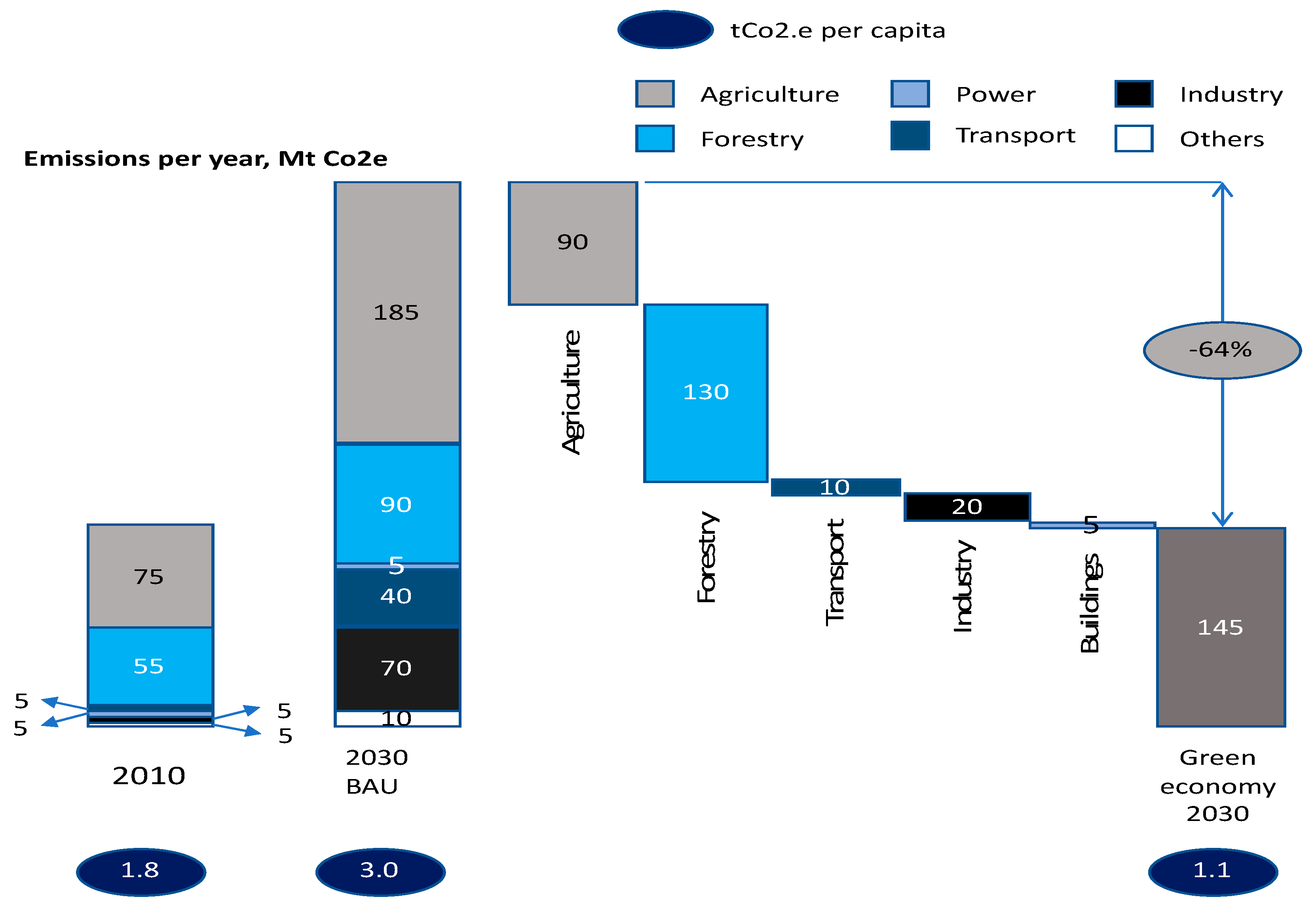
Carbon Emission by Source

Most carbon emissions in Ethiopia emanate from the agriculture sector, land-use change and forestry, as shown in Figure 2. Most of the emissions from the agriculture sector come from livestock. This includes enteric fermentation, manure left on pasture, and manure applied on soil. Emissions from land-use change and forestry include emission due to forest clearance and land-use conversion for smallholder agricultural expansion, promotion of large-scale agriculture, human settlement and authorized and unauthorized logging. Emissions from unsustainable extraction of fuelwood also are typically included within forestry; however, in the subsequent analysis, fuelwood will be considered separately.

Figure 2 shows that livestock accounts for 74.86 million tons (54.53 percent of total emissions), and forestry and firewood together emit 52.8 tons of carbon (38.46 percent of total carbon emissions), respectively. In contrast, the use of petroleum (fuel and kerosene) accounts for only 6.28 percent (i.e., 8.62 million tons of carbon) of overall emissions. Emissions from fertilizer use in the agriculture sector are based on 650,000 tons of fertilizer used in 2012 [10].

Each of the carbon emission sources mentioned above results from either direct consumption by households or use of intermediate inputs in the production of other goods and services. Using statistics on total outputs and inputs of different sectors in the Ethiopian economy, we can compute the direct and indirect carbon intensities and emissions shown in

Table 1. Carbon Intensity by Group of Products.

Product Group	Carbon Intensity (Tons of CO2) Per Millions of Birr of Final Demand
Crops and vegetables	21.7
Livestock	1231.6
Forestry	15.8
Firewood	1937.7
Fishery	9.7
Coal	1725.8
Other mining	6.5
Food processing	183.0
Textile and leather	44.0
Wood and paper products	2.6
Fuels (petroleum other than Kerosene)	196.7
Kerosene	262.0
Chemicals	7.4
Fertilizer	184.0
Non-metal minerals	23.8
Metals and metal products	20.5
Machinery and Equipment	2.2
Vehicles	2.3
Other manufacturing	4.3
Electricity	33.5
Water	36.5
Construction and real estate	12.4
Trade	2.7
Transport	47.5
Hotel	106.1
Communication	11.4
Financial and business services	0.6
Public administration, education, health, and other services	12.7

Source: Authors’ calculation based on the 2010/11 Ethiopian Social Accounting Matrix.

that result from the different sources of carbon emissions. (The mathematical formula used to arrive at the figures presented in Table 1 is given in Appendix C.) Table 1 shows that firewood, coal, and livestock have respectively the highest carbon intensity as measured by tons per million birr of final demand. Kerosene, petrol and fertilizer are a second set of product groups with significant carbon intensity.

The incidence of carbon price on households depends on the carbon content of their consumption, among other factors. Figure 3a describes the carbon emission due to indirect consumption of petroleum fuels, not including kerosene. Petroleum fuels consumption and the resulting emissions are higher as a proportion of a given consumption for richer and urban households. However, as can be seen in Figure 3b the pattern becomes less clear if we consider the consumption of kerosene. Because urban households tend to be more dependent on modern transport, they are more intensive consumers of petroleum fuels. They utilize electricity in addition to kerosene for cooking and lighting purposes. Rural households, on the other hand, lack adequate access to electricity. As a result, they rely more on kerosene for lighting and cooking purposes. The overall fuel (petroleum and kerosene) intensity of consumption of households tends to be similar across categories of households.

3. Methodology for Assessing the Impacts of Carbon Pricing in Ethiopia

3.1. Modeling Framework

This study relies on a recursive dynamic Computable General Equilibrium (CGE) model. It is an extension of the Computable CGE model developed by the International Food Policy Research Institute (IFPRI). The model is formulated as a set of simultaneous linear and non-linear equations that simulate the behavior of consumers and producers across the economy, as well as the functioning of the economy in which these agents operate. (More details about the model are included in Appendix A.) The model can be used to assess the impacts of carbon pricing by tracking, in detail, various transmission mechanisms within and across sectors. The model describes market equilibrium conditions, macroeconomic balances, and dynamic updating equations. Given the nature of our input data, we run all the model scenarios over a period starting in 2018 and ending in 2030.

3.2. Baseline Scenario

Analyzing the impacts of a carbon tax requires a comparison of the performance of the economy with the carbon tax vis-à-vis a Business-As-usual (BAU) case without the carbon tax. Ethiopia’s current tax system has direct taxes (income tax, profit tax, rental tax, etc.) and indirect taxes in the form of Value Added Tax (VAT) (which is 15%), Excise tax, Turn-over tax, and customs duty. There are currently no carbon taxes. Moreover, electricity and kerosene are exempt from VAT and Turn-Over taxes. Our baseline scenario is based on the growth plan embedded in GTP II [11]. We assume that the investment programs, tax policy, and environmental policies in GTP II will take place. This includes all environmental polices embedded in the CRGE Strategy [6]. The economic growth rate under the BAU scenario that we utilize is recorded in the first two years of the GTP II period (i.e., a GDP growth rate of 7.6 percent).

3.3. Policy Scenarios

The policy scenarios included in the current study differ from the BAU not only due to the imposition of a carbon tax but also due to a set of decisions regarding (i) what sources of carbon to tax, (ii) the time path of carbon prices, and (iii) how to use money that is raised through the carbon tax. Decisions taken on each of these elements will imply different policy impacts on the economy vis-à-vis the baseline.

3.3.1. What Sources of Carbon to Tax

As shown in Figure 2, most of the carbon emission in the country comes from the agriculture sector. This implies that any tax that will put a significant dent on emission would have to address the agriculture sector. However, there are two reasons why this would be undesirable and difficult to implement. The sources of emissions from agriculture and forest land use are diverse and diffuse. This makes these sources difficult to tax without extensive, costly, and untested measurement, reporting, and verification (MRV). Note that imposing a carbon tax merely on agricultural and forest outputs is not possible because the carbon intensity of outputs may substantially differ across suppliers and regions of the country. In addition, most of the agricultural activity in the country is undertaken by smallholder farmers engaged in subsistence agriculture. Burdening them with a carbon tax, even if it could be figured out how to do so, would have adverse distributional consequences.

In contrast, taxing fossil fuels has the inverse pros and cons of taxing agricultural emissions. It can easily be administered by imposing a tax on fuel importers. In other words, it does not involve significant levels of MRV measures. Moreover, it is an effective approach for taxing the informal sector. In addition, it can easily be linked with other existing taxes in the overall fiscal system. Therefore, although fossil fuels make only a small contribution to total GHG emissions in Ethiopia (a bit more than 6 percent, as noted in Section 3), this study focuses on putting a price on the carbon emitted from fossil fuels. An important follow-up task beyond the scope of this study is to give much deeper consideration to what policies, beyond carbon pricing, can effectively mitigate GHG emissions from agriculture and forestry.

How kerosene is factored in carbon tax analysis has important implications due to two seemingly countervailing reasons. On the one hand, kerosene is an alternative cooking energy to fuelwood; taxing it may backfire by increasing consumption of fuelwood which could result in more GHG emissions as well as worse indoor air pollution. On the other hand, exempting kerosene from a carbon tax could lead to tax evasion through reclassification of other fuels as kerosene. We have carried out our policy comparisons both with and without kerosene. However, in this report, we include only results from the analysis with kerosene taxed. The results with kerosene exempted are available on request.

3.3.2. The Time Path of Carbon Prices

Another important factor is deciding what level of tax to impose and how the tax rate evolves over time. The range of carbon prices being used is from $1 per ton to over $125 per ton, there are many examples in the range of $5 to $30 per ton [1]. Accordingly, we have analyzed three possible cases. The first entails imposing a low tax of about $5 per ton throughout the time period of the analysis (2018–30). The second entails imposing a higher tax rate of $30 per ton initially and maintaining that rate throughout 2018–30. In the third case, the tax rate starts at $5 per ton and then steadily grows over the study period until it reaches $30 per ton in 2030. Although we have run our model based on all three tax design cases, in this report, we include only the results from the third case “starting low and steady growth” for various reasons: (i) it is a realistic assumption of how carbon pricing might be implemented in practice; (ii) a carbon price of $5 per ton has little relevance by 2030 when countries’ NDCs targets need to be met; and (iii) a carbon price of $30 per ton now can be considered excessive if compared with other developing economies.

While the carbon price is to function as a tax on carbon emissions, in practice it needs to be imposed on the fossil fuels themselves; therefore, it is necessary to convert the carbon tax rate to fuel-specific taxes based on their respective carbon contents. Imposing a $5 price on carbon is equivalent to a 2.23 percent tax on petroleum fuels, based on the fuel prices utilized in the study. ($5 per ton of CO₂* 3.5 ton of CO₂ per ton of fuel = $17.5 per ton of fuel. Since 1176 L is equal to 1 ton of oil, this is equivalent to $0.015 per liter of fuel. Using the current price of $0.67 L of fuel, then $5 price is equivalent to 2.23% tax.) Similarly, a $30 price on carbon is equivalent to a 13.4 percent tax on petroleum fuels given the assumed prices.

As of 2015, 2.68 million tons of various oils were used in the country, according to the International Energy Agency. Using the average conversion factor of 3.5 tons of CO₂ per ton of oil, the CO₂ emissions in 2015 from use of fossil fuels was 9.54 million tons. Consequently, in 2015, a $5 price on carbon would have raised $47.7 million, while a $30 price on carbon would have raised $286 million.

4. How to Use the Increased Carbon Revenue

The structure of the model we employ is such that the equilibrium in the economy is consistent with the government budget constraint. The revenue from carbon tax increases government revenue. The government has to use the money to reduce borrowing, reduce debt, increase spending, or reduce other taxes. Consequently, how to utilize the increased government revenue becomes a relevant policy issue. After discussions with many policy-making units and other relevant stakeholders, we decided to evaluate five options for how to use the money that is raised through the carbon tax:

• STAX—A scenario where we adopt uniform reduction of sales taxes for intermediate and final commodities.
• TRANS—A scenario where the increased government revenue is used as a lump-sum transfer payment to all households. Lump-sum transfer payments follow the same pattern of existing allocation of government transfers to each type of household. The proportion of transfers to household types is maintained. (As indicated in Appendix A, the Social Accounting Matrix has 15 types of households. The initial share refers to the government transfer to each type of household relative to overall government transfer to households. The basic premise in this scenario is that the current transfer scheme reflects the weight the government puts on the welfare of each type of household.)
• SAVINGS—A scenario where the money from carbon tax is directed to the overall saving pool where it can then be invested in the most profitable sectors.
• DTAX—A scenario where the money from carbon tax is transferred to taxpaying households in the formal sector. This is done in the form of uniform reduction of direct taxes (personal income tax).
• CORPOR—A scenario where the money is used to encourage investment by firms. This is achieved by uniform reduction of business income tax.

We compare the results from imposing the specified carbon tax with these different uses of revenues to the BAU scenario.

5. Modeling Results

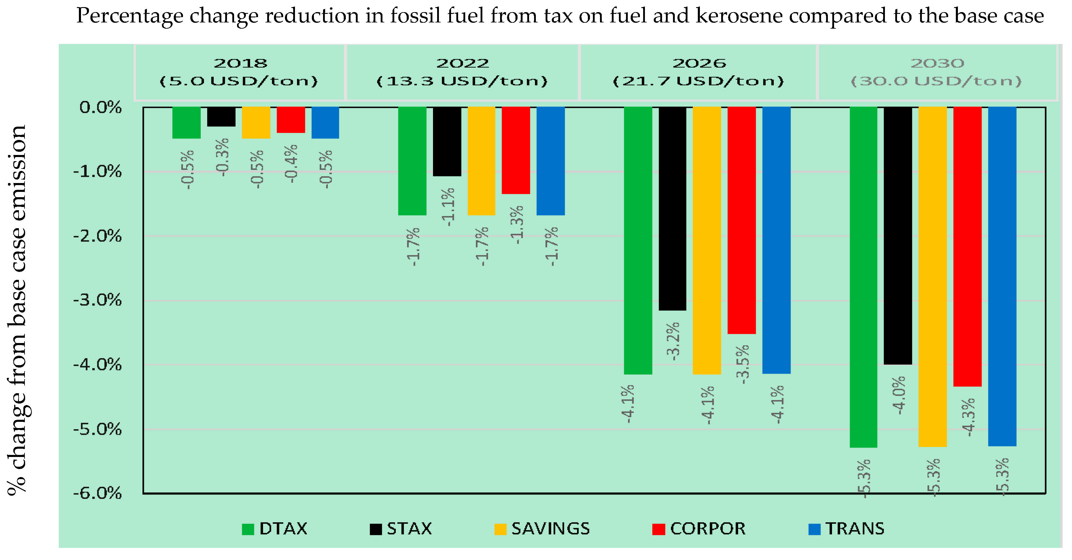
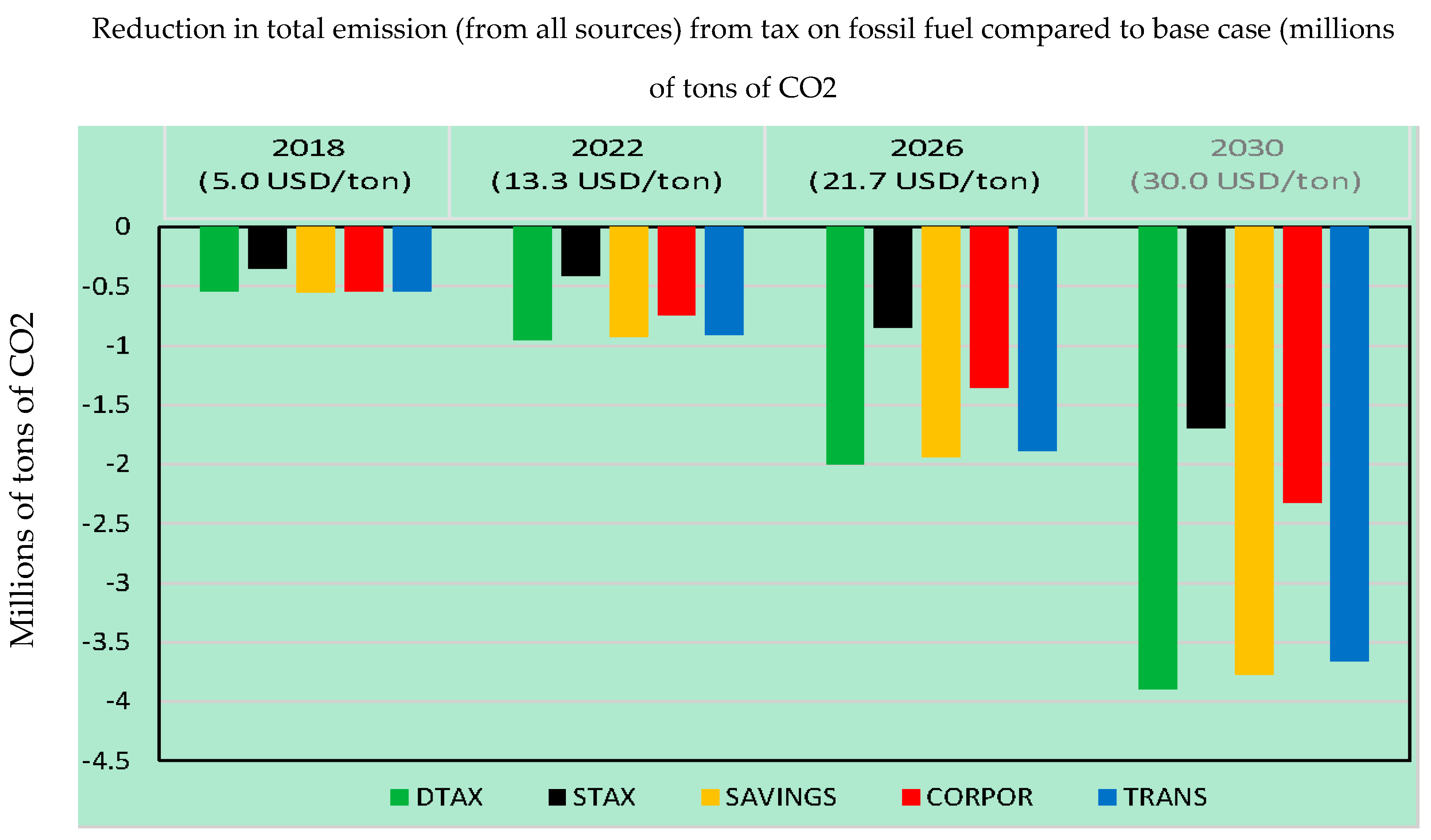
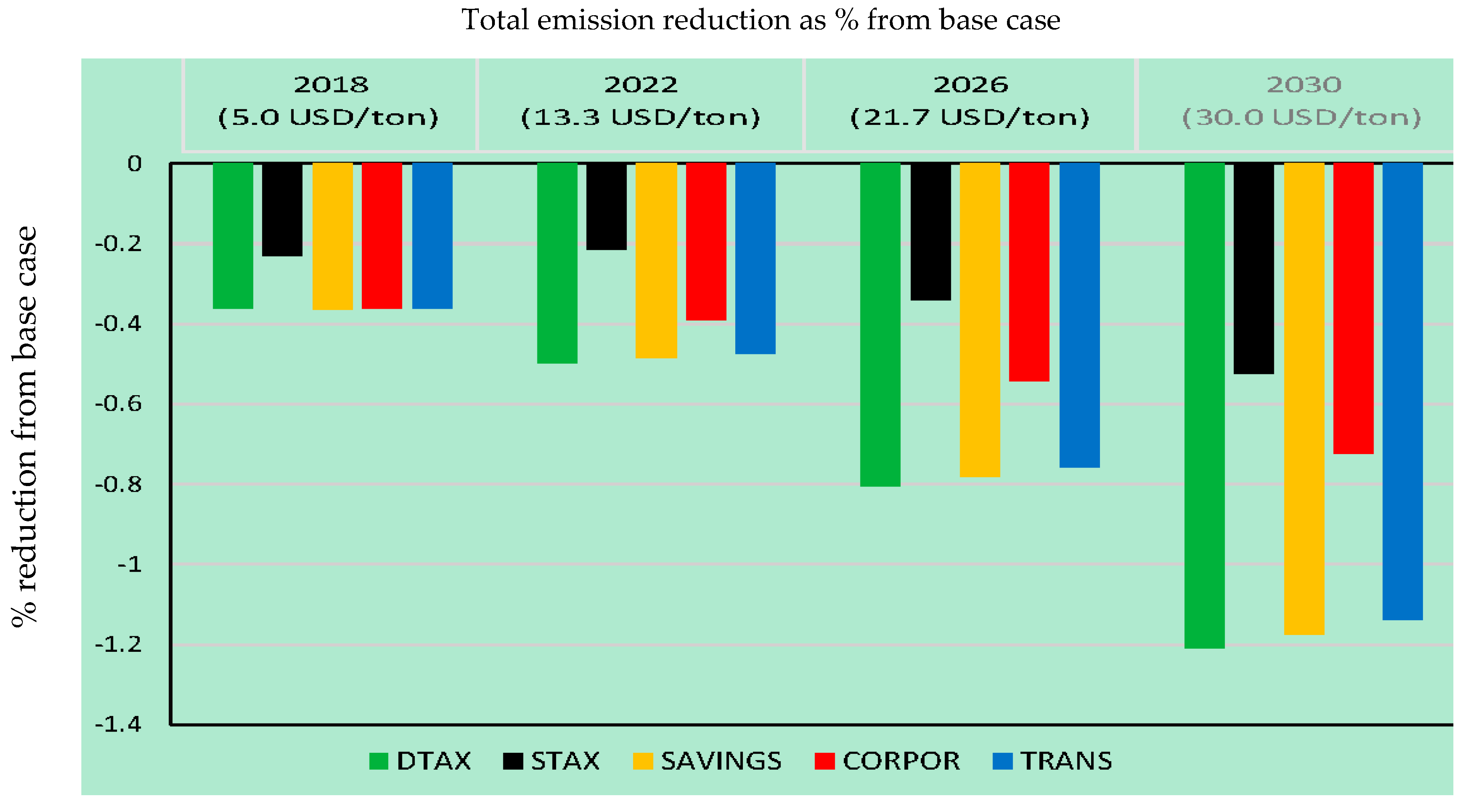
5.1. Impact on Emissions

Figure 4 and Figure 5 present summary results of changes in emissions across the different scenarios. The figures show that, as expected, emission reductions increase over time as the price on carbon increases. Depending on the recycling scenario, the reduction ranges from 1.1 million tons to 1.5 million tons relative to BAU in 2030, when the carbon tax reaches its maximum value. The differences across scenarios are due to the differences in growth of the economy due to the different revenue recycling mechanisms considered, which in turn influence the demands for fossil fuels.

Comparing across the scenarios, the least emission reduction is achieved in the sales tax (STAX) reduction scenario. This is because its effect on the general economy results in the least growth impact. Direct tax reduction (DTAX), on the other hand, leads to more significant reductions in emissions.

Similar comparisons follow when we compare the resulting reductions in emissions from all emission sources. These will be larger than the reductions in emissions in fossil fuels, because the changes in fuel prices will have effects on the quantities of other emissions-producing activities in the economy. By 2030, as compared to the base case, the STAX reduction scenario will lead to a reduction of total emission by 1.7 million tons while the DTAX reduction scenario will lead to a reduction of total emission by about 3.8 million tons (see Figure 6 and Figure 7).

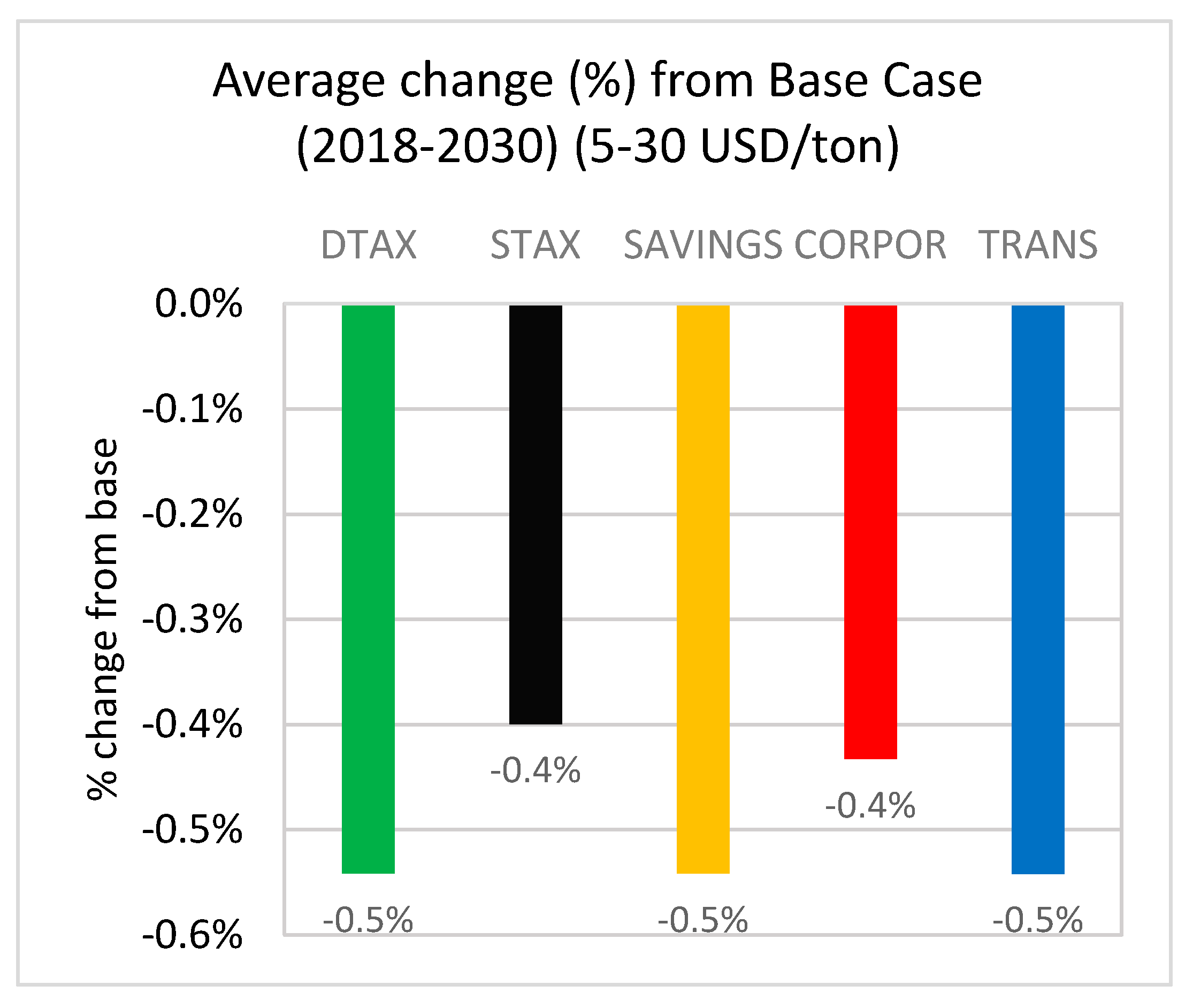
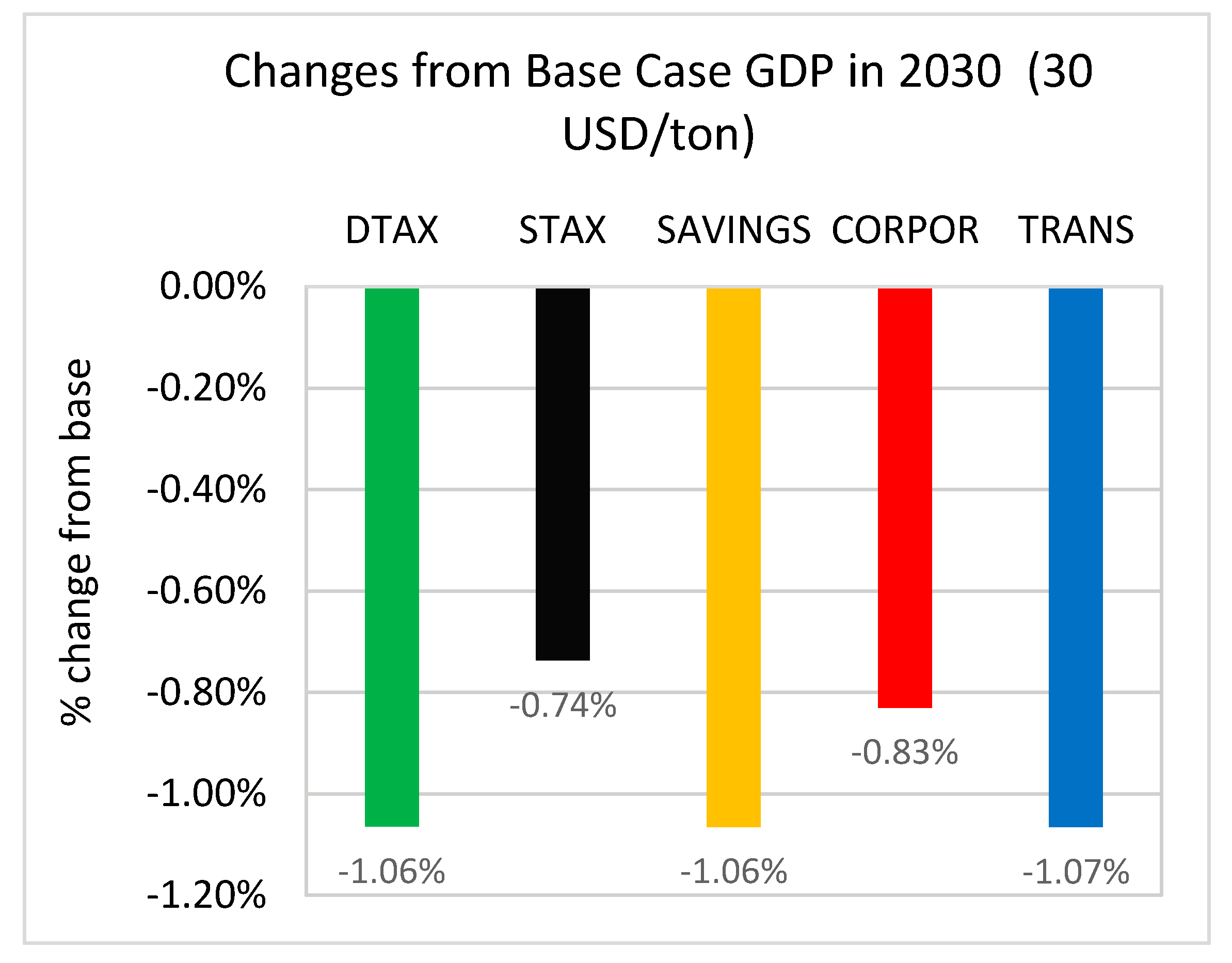
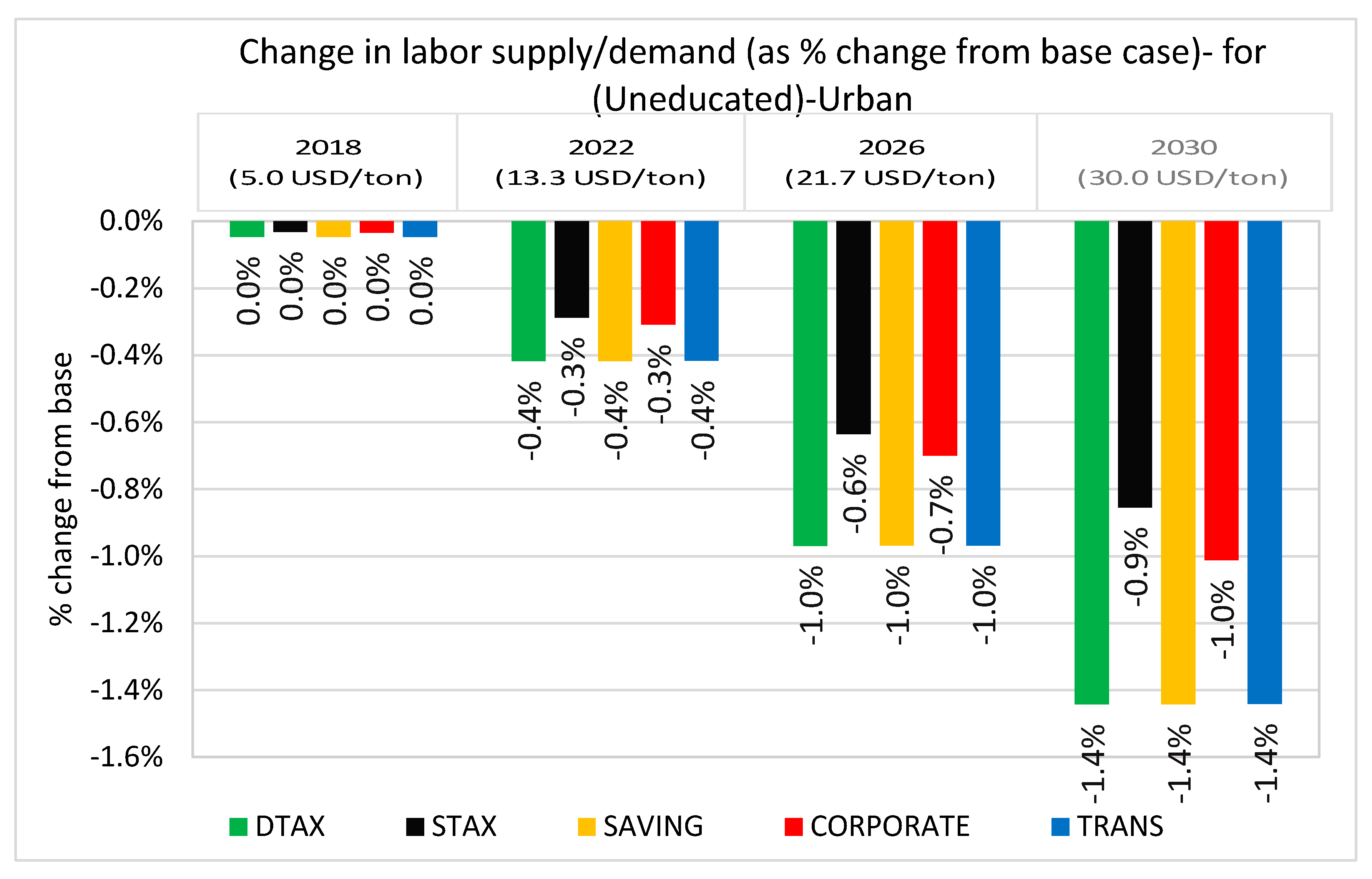
5.2. Impacts on the Economy

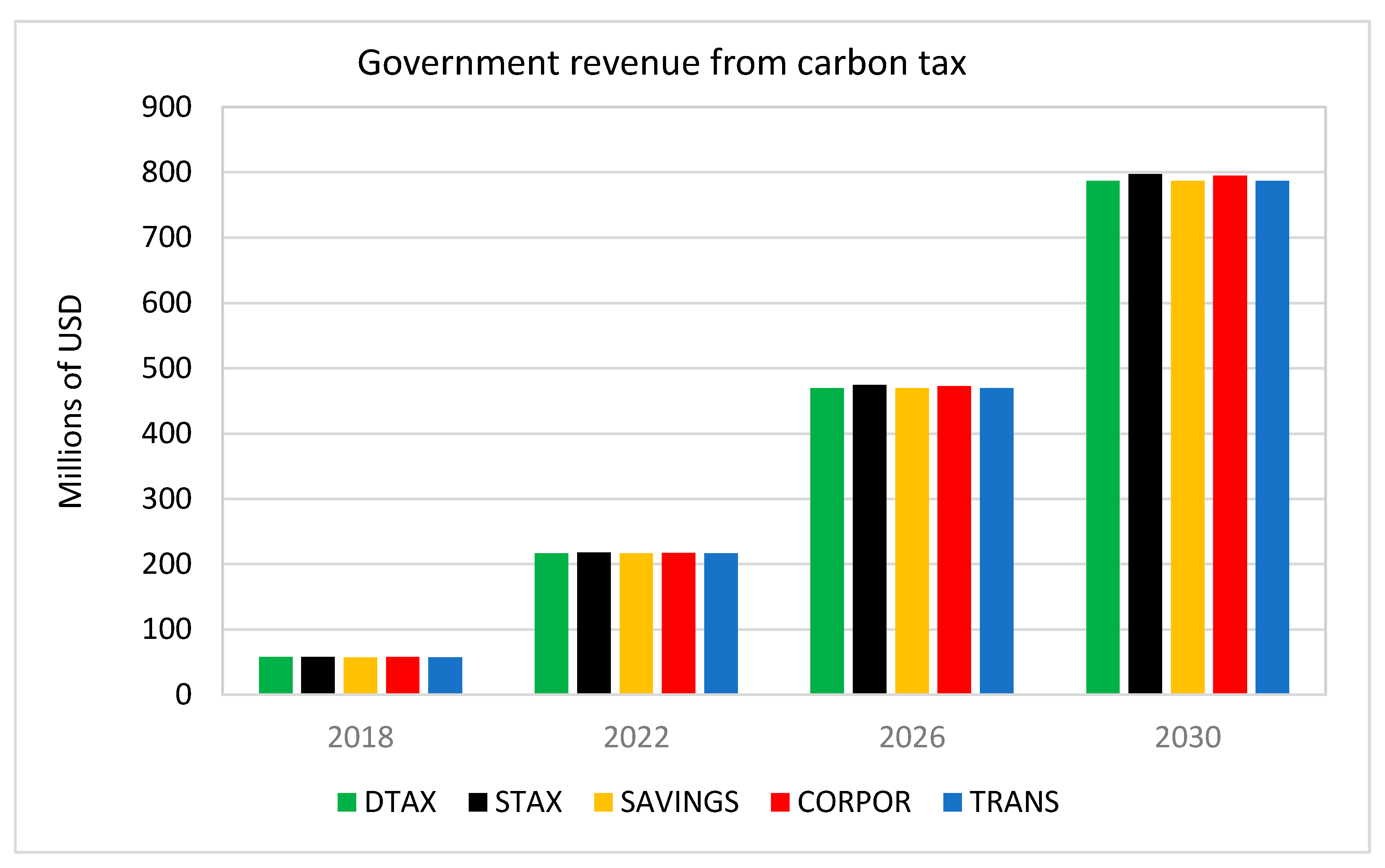
The assumed time path of carbon prices has a fairly modest effect on the growth of GDP (Figure 8 and Figure 9). In BAU, GDP is much higher in 2030 than in 2015 given the assumed growth rates for the economy. The same is true in the policy scenarios; the different tax and recycling combinations only slow growth by a little over the study period. GDP in 2030 is about 1 percent lower compared to BAU in almost all scenarios. Average GDP growth is from 0.38 to 0.52 percentage points lower with the carbon pricing than under BAU, depending on the chosen scenario. This is a small decrease in the growth rate of 7.6 percent per year in BAU.

A cut in either sales or corporate tax leads to smaller negative effects on GDP compared to the other policy scenarios. The reason is that lower sales tax reduces cost of goods and services and stimulates demand across income groups. Lower business tax reduces the cost of capital which encourages investment and therefore employment and production. Both tax reductions end up reducing existing distortions in the economy. That, in turn, will lessen the amount of emission reduction from the carbon tax.

The scenario in which personal income tax is reduced leads to a larger decrease in the growth of economic activity. The reason is that professional and educated labor—the types of workers paying the personal income tax—is assumed to be fully employed. Reducing income tax therefore increases neither labor supply nor economic activity.

5.3. Fiscal Impacts

Because the government account should balance, and government expenditures are treated as fixed in the analysis, the government recycles the entire change in revenues in each of the five policy scenarios. To assess the amount of revenue raised through carbon pricing in each scenario, we first calculate the amount of fuel imported each year. We then multiply the fuel import by the emission factor (i.e., emission per unit of fuel) to arrive at a figure for total emissions, and then use the assumed carbon tax rate to calculate total carbon tax revenue.

The revenue generated in 2030 ranges from $786 million under the direct tax scenario to $798 million under the sales tax reduction scenario (Figure 10). The differences in revenue among scenarios are due to the differences in economic growth which, in turn, affect the demand for fuel.

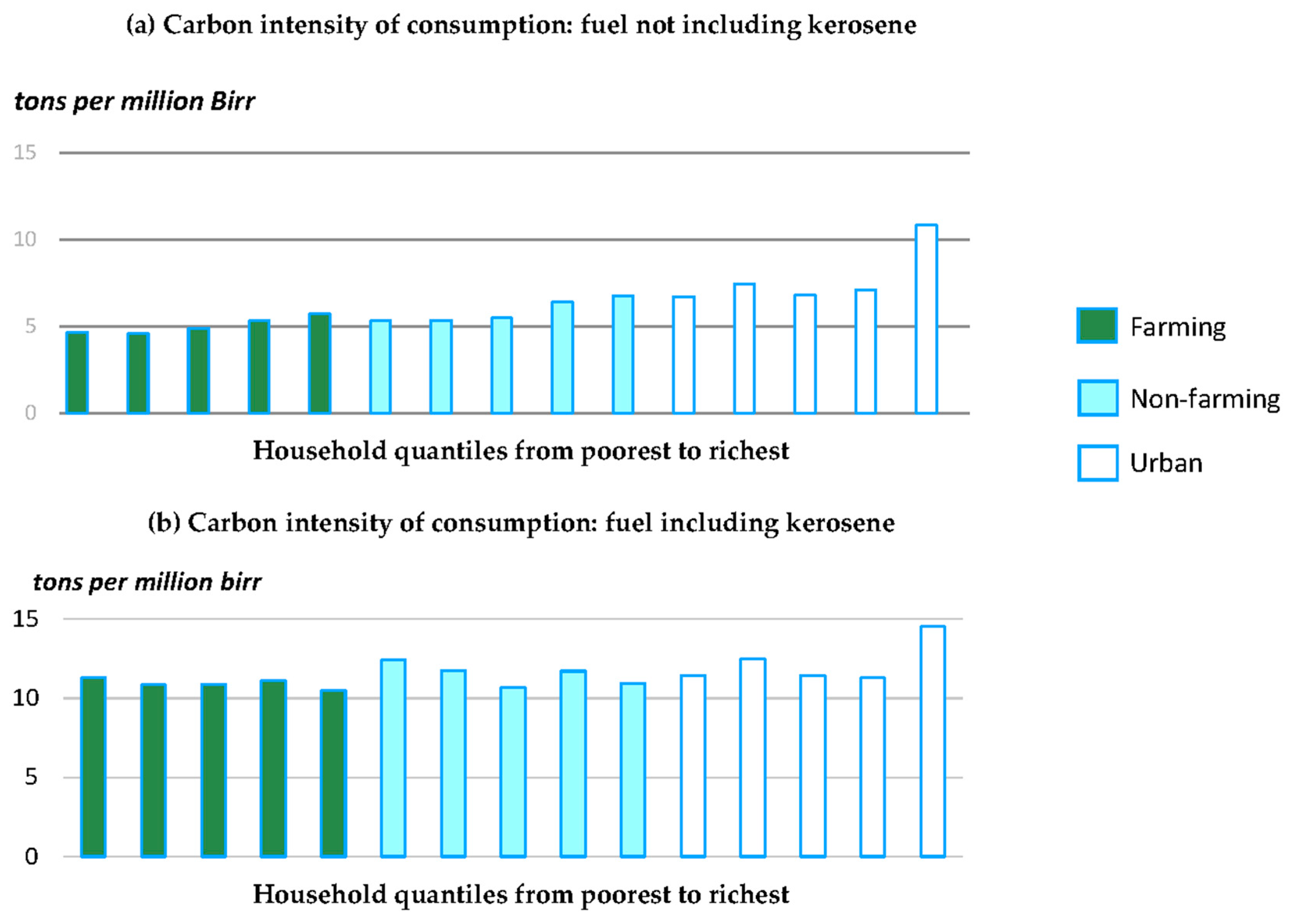
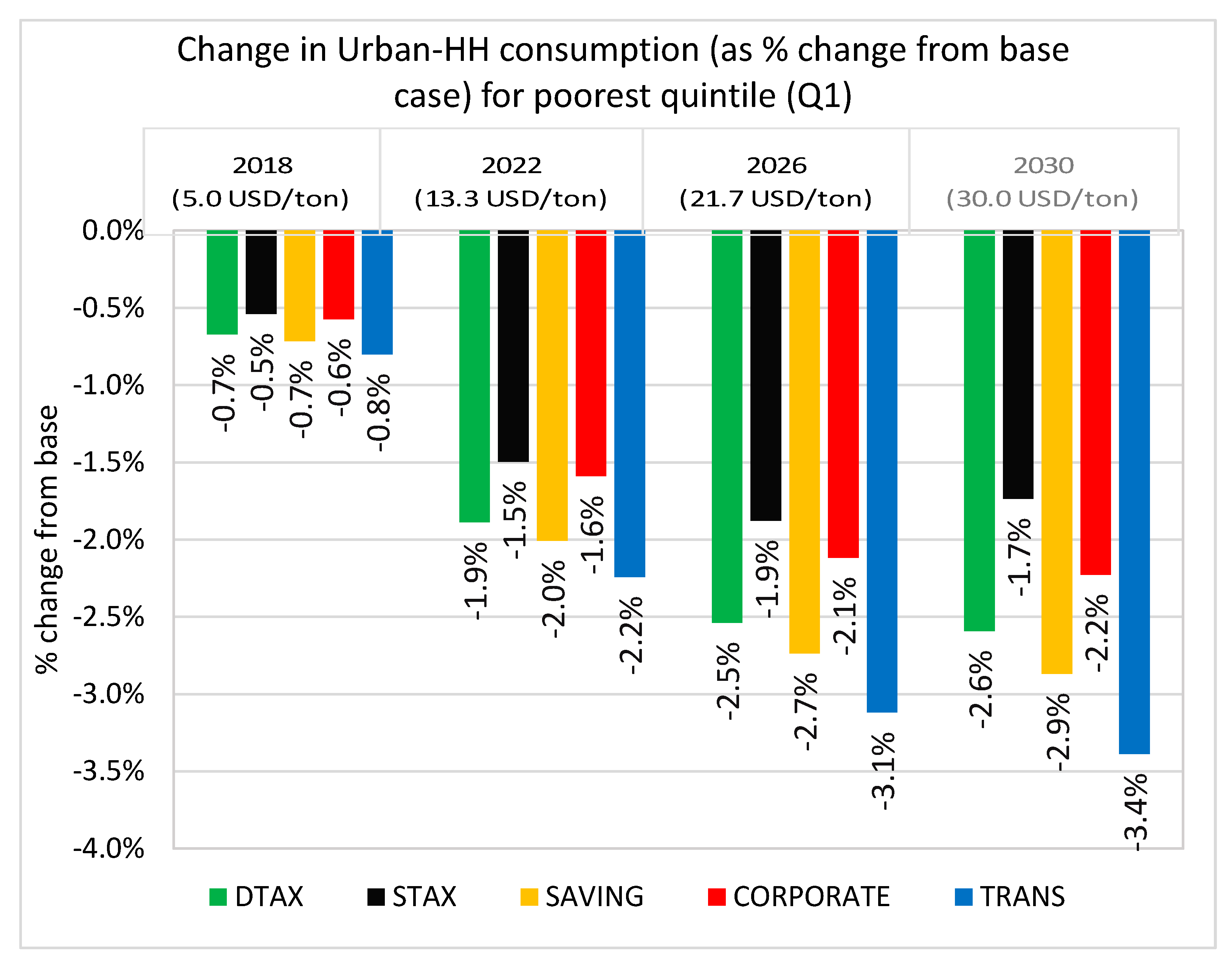
5.4. Distributional Impacts

Although the impact of the carbon tax on overall economic growth is one indication of the economic consequences of the policy, a much clearer understanding of the full implications for economic well-being comes from looking at the impacts across heterogeneous households based on factors such as their location (urban, rural) and their abilities (skilled, unskilled). Households receive income from wages (employment), returns on land for which they have the right of use, returns on capital they own, and income transfers. The implication of a carbon tax on a household’s welfare, therefore, depends on how it affects each of these sources of household income.

In this subsection, we highlight the heterogeneous impacts on labor demand (employment) and household consumption. Figure 11 and Figure 12 provide the difference in employment trend of low-skilled individuals located in the urban and rural sector. The carbon tax on fuels increases the price of goods reliant on fuel-using transport. As a result, it shifts demand away from those goods towards others. Sectors that are transport and thus fuel dependent include the service and manufacturing sectors. Both sectors are overwhelmingly concentrated in urban areas. As a result, there will be a decrease in urban unemployment (Figure 11) among low-education workers. Because we assume full employment for high-skill individuals, they adjust to the carbon tax through a wage decrease rather than an employment decrease.

The agriculture sector, on the other hand, does not rely as heavily on transportation. Therefore, it benefits from an increase in demand relative to other goods. This, in turn, increases the employment potential of rural unskilled labor compared to their urban counterparts. Figure 12 indicates that there is almost no effect on employment across scenarios in rural areas compared to the base case scenario. (Note that in the base case scenario, employment of low-skilled individuals in urban areas is assumed to be 4,186,322 in 2018 and 6,290,527 in 2030. Similarly, employment of low-skilled individuals in rural areas is assumed to be 38,516,966 in 2018 and 54,301,218 in 2030.)

The tax has differing impacts on the consumption of the lowest quintile households in urban and rural areas. In urban areas (Figure 13), the main source of income for poor households is employment income (wages). As the sectors that poor households work in (services and industry) are affected more by the carbon tax, their income decreases due to either increased unemployment or a decrease in wage. The implication for economic welfare depends on the scenario: revenue recycling under STAX and CORPOR leads to smaller decline in consumption than others because there is less impact on the economy. TRANS, on the other hand, limits the decline in consumption by transferring resources to poorer households.

In rural areas, the ‘almost non-existent’ effect of the carbon tax on agriculture means that employment is not really affected (Figure 14). In addition, the tax slightly increases the return to land owned by rural households. The combination of these two effects implies that the impact of the carbon tax on the consumption of poor rural households is minimal. It is worth noting that, ex ante, one would expect that the poor will fare better under the transfer scenario. However, the result shows the opposite. There are a couple of reasons for this. First, the transfer scenario does not restrict transfers to poor households. Since a large share of transfers are made to urban/richer households, it limits the extent to which the aggregate transfer can reduce poverty and inequality. Second, the slowdown in economic activity under the transfer scenario introduces unemployment/wage reduction that affects welfare directly. Another way to understand the result under the transfer scenario is that one needs to restrict the transfer to poor households in order to achieve a meaningful reduction in poverty and inequality.

6. Concluding Remarks

Over 90 percent of Ethiopia’s GHG emissions comes from sources other than fossil fuels. This is because (a) energy use in general is relatively low, including in transport, although it is expected to grow as the economy expands; (b) most of Ethiopia’s electricity comes from hydro; and (c) biomass remains the overwhelming choice of energy source for cooking. Consequently, application of carbon pricing to fossil fuels use in Ethiopia necessarily will have a somewhat limited effect on total GHG emissions.

Nevertheless, since motorization increases as incomes rise, the carbon price on fuels can contribute to mitigating a “lock-in” of high levels of individual vehicle use and high demand for road expansion by limiting vehicle use and creating support for expanding well-performing public transit and smaller, efficient cars in more densely populated areas. The carbon price on fossil fuels limits fuel use and associated GHG emissions cost effectively compared to what might result from a patchwork of different regulatory standards on various emissions sources. It creates incentives for increasing energy efficiency including in transport choices. By moving away from carbon, Ethiopia may benefit in the long run from energy efficiency and relatively cheaper sources of energy, providing a competitive advantage over those countries that did not make the transition and have locked-in inefficient technologies. In addition, revenue-neutral reductions in other taxes can be made to spur investment and productivity gains.

Regarding economic impacts, GDP continues to grow substantially, albeit at a modestly lower rate. The direct effect of the carbon price is likely to be felt more by higher-income households since they are more intensive consumers of fossil fuels. Indirect effects through adjustments in the economy to higher fuel prices can lead to modestly slower growth for the urban poor, but the size of that effect will depend on how carbon revenues are recycled. Because the rural poor are not intensive users of fossil fuels, and the economic adjustments to carbon pricing may have limited impact on the agriculture sector, the rural poor are likely to face little impact from it. As we have shown, some portion of carbon tax revenues can be used to soften impacts on the poor.

A significant impact for Ethiopia of applying a carbon price to fossil fuels is that substantial revenues can be generated—up to $800 million per year by 2030. Part of the revenue could be used to finance other carbon mitigation activities, with a focus on those activities that have high societal co-benefits that strengthen the rationale for such public expenditures. Three such types of expenditures seem to stand out:

• Increase reforestation activities over and beyond what might be financed internationally through the country’s REDD program. Investments in forest recovery can provide important ecosystem benefits, including soil and watershed protection and habitat for valued species, as well as expended carbon storage. This use of revenues is well aligned with the pillars of the CRGE [6].
• Provide technology-neutral subsidies to increase affordability of improved cookstoves that use biomass fuel more efficiently or not at all, thereby reducing time spent collecting fuelwood and the substantial adverse health impacts of indoor smoke, especially for women and girls. Even if affordable alternatives to fuelwood for cooking take time to scale up in rural areas, cookstoves with improved fuel efficiency and improved ventilation can generate some improvement of indoor air quality, while reducing the level of unsustainable fuelwood harvest and the production of black carbon. Increasing access to cleaner cooking also is a pillar of CRGE [6].
• Find ways to increase the efficiency of fossil fuel use in urban transport, thereby slowing its growth and the corresponding increase in GHG emissions. This could be done through investment in more fuel-efficient and less-polluting multiple-rider transit vehicles in urban areas, thereby mitigating another major public health challenge. It would also be beneficial to use a portion of carbon pricing revenues to increase oversight of fuel quality.

As noted, GHG emissions from fossil fuel combustion are only a limited part of the story in Ethiopia. Other significant emissions sources include land clearing for expanding agriculture, and unsustainable consumption of wood-based fuels for cooking and heating. To provide a complete picture of how carbon pricing and other policies can manage Ethiopia’s emissions in accordance with its national commitments, it is necessary to go beyond the scope of this study to consider what combinations of pricing and other measures can be effective in limiting emissions from the agriculture and forest sectors, including fuelwood in the latter. Using price-based measures to restrict land clearing and fuelwood use is challenging, though not impossible. Further research can address land taxes that encourage land rehabilitation, reforestation, and maintenance of natural forests, as well as land clearing taxes. Another fruitful avenue for investigation is how changes in current industrial development and import substitution policies could lower the cost of access to more energy-efficient and less-polluting technology and capital.

Finally, the model does not explicitly differentiate between employment and output from informal and formal sectors of the economy. The model also does not include the possibility of lasting structural unemployment for part of the labor force. Both of these considerations can substantially affect the conclusions of a carbon tax impact analysis.

Although the importance of these issues has been noted for some time, the practical capability to deal with them using larger-scale CGE models is still developing. Markandya, González-Eguino, and Escapa [12] developed a CGE model for Spain including informal employment. Mirhosseini, Mahmoudi, and Valokolaie [13] use a variant of that model for Iran. Bento, Jacobsen, and Liu [14] apply a much more aggregated model with informal employment and different types of energy usage in the informal sector to China and India. These studies indicate that a significant informal sector can lead to lower adverse impacts on the economy of carbon pricing. However, all three of the studies use static, long-run equilibrium models that by their nature cannot capture the effects of ongoing adjustment over time to a potentially changing carbon tax.

Employment impacts of a carbon tax depend on the types and extent of pre-existing distortions in labor markets, how the carbon tax may alter the sectoral content of GDP, and how recycling of carbon tax revenues may affect the after-tax cost of hiring for firms. Markandya [15] provides a very useful review of these considerations. Labor market distortions can be the result of wage rigidity, labor market segmentation, or search costs [16,17,18,19]. As with the inclusion of informality, methods for including labor market structural rigidities in CGE models are still evolving. Relaxing the limitations noted here with a more advanced CGE model would represent a valuable direction for follow-up work.

References

1. World Bank. State and Trends of Carbon Pricing 2019; World Bank: Washington, DC, USA, 2019. [Google Scholar]
2. New Climate Economy. The Sustainable Infrastructure Imperative: Financing for Better Growth and Development; World Resources Institute: Washington, DC, USA, 2016. [Google Scholar]
3. Gebregziabher, G.; Abera, D.A.; Gebresamuel, G.; Giordano, M.; Langan, S. An Assessment of Integrated Watershed Management in Ethiopia; International Water Management Institute (IWMI): Colombo, Sri Lanka, 2016; Volume 170. [Google Scholar]
4. Haileselassie, A.; Hagos, F.; Mapedza, E.; Sadoff, C.W.; Awulachew, S.B.; Gebreselassie, S.; Peden, D. Institutional Settings and Livelihood Strategies in the Blue Nile Basin: Implications for Upstream/Downstream Linkages; IWMI: Colombo, Sri Lanka, 2009; Volume 132. [Google Scholar]
5. Coady, D.; Flamini, V.; Sears, L. The Unequal Benefits of Fuel Subsidies Revisited: Evidence for Developing Countries; International Monetary Fund Working Paper 15/250; International Monetary Fund: Washington, DC, USA, 2015. [Google Scholar]
6. FDRE. Ethiopia’s Climate-Resilient Green Economy: Green Economy Strategy; Federal Democratic Republic of Ethiopia: Addis Ababa, Ethiopia, 2011. [Google Scholar]
7. High-Level Commission on Carbon Prices. Report of the High-Level Commission on Carbon Prices; License: Creative Commons Attribution CC BY 3.0 IGO; World Bank: Washington, DC, USA, 2017. [Google Scholar]
8. Liu, A. Tax evasion and optimal environmental taxes. J. Environ. Econ. Manag. 2013, 66, 656–670. [Google Scholar] [CrossRef]
9. Angelsen, A. Policy Options to Reduce Deforestation. In Realising REDD+: National Strategy and Policy Options; Angelsen, A., Ed.; Center for International Forestry Research: Bogor, Indonesia, 2009. [Google Scholar]
10. Rashid, S.; Tefera, N.; Minot, N.; Ayele, G. Fertilizer in Ethiopia: An Assessment of Policies, Value Chain, and Profitability; IFPRI Discussion Paper 01304; International Food Policy Research Institute: Washington, DC, USA, 2013. [Google Scholar]
11. FDRE. The Second Growth and Transformation Plan (GTP-II); Ethiopian National Planning Commission: Addis Ababa, Ethiopia, 2015.
12. Markandya, A.; González-Eguino, M.; Escapa, M. From Shadow to Green: Linking Environmental Fiscal Reforms and the Informal Economy. Energy Econ. 2013, 40, S108–S118. [Google Scholar] [CrossRef]
13. Mirhosseini, S.; Mahmoudi, N.; Valokolaie, S. Investigating the Relationship between Green Tax Reforms and Shadow Economy Using a CGE Model—A Case Study in Iran. Iran. Econ. Rev. 2017, 21, 153–167. [Google Scholar]
14. Bento, A.; Jacobsen, M.; Liu, A. Environmental Policy in the Presence of an Informal Sector. J. Environ. Econ. Manag. 2018, 90, 61–77. [Google Scholar] [CrossRef]
15. Markandya, A. Environmental Taxation: What Have We Learnt in the Last 30 Years? In Environmental Taxes and Fiscal Reform; Castellucci, L., Markandya, A., Eds.; Macmillan: Basingstoke, UK, 2012; pp. 9–56. [Google Scholar]
16. Devarajan, S.; Go, D.S.; Robinson, S.; Thierfelder, K. Tax Policy to Reduce Carbon Emissions in a Distorted Economy: Illustrations from a South Africa CGE Model. BE J. Econ. Anal. Policy 2011, 11. [Google Scholar] [CrossRef]
17. Guivarch, C.; Crassous, R.; Sassi, O.; Hallegatte, S. The Costs of Climate Policies in a Second-Best World with Labour Market Imperfection. Clim. Policy 2011, 11, 768–788. [Google Scholar] [CrossRef]
18. Hafstead, M.A.C.; Williams, R.C., III. Unemployment and Environmental Regulation in General Equilibrium. J. Public Econ. 2018, 160, 50–65. [Google Scholar] [CrossRef]
19. Hafstead, M.A.C.; Williams, R.C., III; Golub, A.; Meijer, S.; Narayanan, B.G.; Nyamweya, K.; Steinbuks, J. Effect of Climate Policies on Labor Markets in Developing Countries: Review of the Evidence and Directions for Future Research; Policy Research Working Paper 8332; World Bank: Washington, DC, USA, 2018. [Google Scholar]
20. Thurlow, J. A Recursive Dynamic CGE Model and Microsimulation Poverty Module for South Africa; International Food Policy Research Institute: Washington, DC, USA, 2008. [Google Scholar]
21. Lofgren, H.; Harris, R.; Robinson, S. A Standard Computable General Equilibrium (CGE) Model in GAMS; Microcomputers in Policy Research 5; IFPRI: Washington, DC, USA, 2002. [Google Scholar]
22. Diao, X.; Thurlow, J. A Recursive Dynamic Computable General Equilibrium Model. In Strategies and Priorities for African Agriculture: Economywide Perspectives; Diao, X., Thurlow, J., Benin, S., Fan, S., Eds.; IFPRI: Washington, DC, USA, 2012; Chapter 2; pp. 17–50. [Google Scholar]
23. Ahmed, H.; Tebekew, T.; Thurlow, J. The 2010/11 Social Accounting Matrix for Ethiopia: A Nexus Project SAM; IFPRI: Washington, DC, USA, 2017. [Google Scholar]
24. NPC. National Economic Accounts Statistics of Ethiopia: Estimates of the 2015/16(2008 EFY); National Planning Commission: Addis Ababa, Ethiopia, 2016.
25. Leontief, W. Environmental Repercussions and the Economic Structure: An Input-Output Approach. Rev. Econ. Stat. 1970, 52, 262–271. [Google Scholar] [CrossRef]
26. Arndt, C.; Davies, R.; Makrelov, K.; Thurlow, J. Measuring the Carbon Intensity of the South African Economy. S. Afr. J. Econ. 2013, 81, 393–415. [Google Scholar] [CrossRef] [Green Version]
Figure 1. The CRGE Strategy’ targes for Low-Carbon Development. Source: [6].
Sustainability 11 04395 g001
Figure 2. The sources of carbon emission in Ethiopia. Source: The livestock and fertilizer data are sourced from FAO (www.fao.org/faostat/en/#data/GT). The forestry and firewood data are from the Environment, Forests and Climate Change Commission (MEFCC) (Mefcc.gov.et/Ethiopia-forest-sector-ghg-emissions, 2017). The data on fuels and kerosene are from the International Energy Agency (IEA) (https://www.iea.org/statistics/statisticssearch/report/?country=Ethiopia&product=oil). Emission factors are from FAO (http://www.fao.org/faostat/en/#data, 2017b), and Intergovernmental Panel on Climate Change (IPCC) (http://www.ipcc-nggip.iges.or.jp/public/2006gl/vol4.html).
Sustainability 11 04395 g002
Figure 3. Carbon intensity of household consumption in Ethiopia due to petroleum fuels. (a) Carbon intensity of consumption: fuel not including kerosene; (b) Carbon intensity of consumption: fuel including kerosene. Source: Authors’ calculation based on the 2010/11 Ethiopian Social Accounting Matrix.
Sustainability 11 04395 g003
Figure 4. Reduction in fossil fuel emission (millions of tons of CO2) from tax on fuel and kerosene compared to the base case.
Sustainability 11 04395 g004
Figure 5. Percentage (%) change reduction in fossil fuel emission from tax on fuel and kerosene compared to base case.
Sustainability 11 04395 g005
Figure 6. Total emission reduction in millions of tons from base case.
Sustainability 11 04395 g006
Figure 7. Total emission reduction as % from base case.
Sustainability 11 04395 g007
Figure 8. Changes from base case average GDP growth rate (2018–2030).
Sustainability 11 04395 g008
Figure 9. Changes from base case GDP in 2030.
Sustainability 11 04395 g009
Figure 10. Government revenue from carbon tax.
Sustainability 11 04395 g010
Figure 11. Changes in labor supply/demand for urban uneducated.
Sustainability 11 04395 g011
Figure 12. Changes in labor supply/demand for rural uneducated.
Sustainability 11 04395 g012
Figure 13. Urban household consumption (poorest quintile Q1).
Sustainability 11 04395 g013
Figure 14. Rural household consumption (poorest quintile Q1).
Sustainability 11 04395 g014