Article

A Framework for Introducing Climate-Change Adaptation in Pavement Management

1
JFK Environmental Services LLC, Upton, MA 01568, USA
2
Department of Civil and Environmental Engineering, University of New Hampshire, Durham, NH 03824, USA
3
School for the Environment, University of Massachusetts-Boston, Boston, MA 02125, USA
*
Author to whom correspondence should be addressed.
Sustainability 2019, 11(16), 4382; https://doi.org/10.3390/su11164382
Submission received: 12 July 2019 / Revised: 7 August 2019 / Accepted: 8 August 2019 / Published: 13 August 2019
(This article belongs to the Special Issue Sustainable Infrastructure Materials and Systems)

Abstract

:
Greenhouse gas emissions have caused global temperatures to rise since the mid-20th century accompanied by sea-level rise (SLR). Temperature increases and SLR-induced groundwater rise have been shown to cause premature pavement failure in many roadway structures. Hybrid bottom-up/top-down (hybrid) adaptation approaches have shown promise by initially investigating an asset’s response to incremental environmental change and then identifying the timing of critical effects for budgetary planning. This improves practitioners’ understanding of the asset’s climate resiliency and informs adaptation-plan development to minimize both cost and risk. In this study, a hybrid approach to pavement adaptation with climate-change-induced temperature and groundwater rise is demonstrated at a case-study site in coastal New Hampshire. The hot-mix-asphalt (HMA) thickness that achieves a minimum of 85% reliability is calculated for 70 combinations of incremental temperature and groundwater rise. Increasing the base-layer thickness improves resiliency against rising temperatures, but rising groundwater diminishes this improvement demonstrating that both HMA and base-layer thickness increases are needed. Thirteen adaptation pathways are evaluated for pavement performance, life-cycle costs, and road-surface inundation over a 60-year pavement management period. A stepwise and flexible adaptation plan is developed that includes HMA overlays with prescribed thickness and application timing, base-layer rehabilitation options, and re-evaluation opportunities.

1. Introduction

Pavements have been historically designed with the assumption that climate is stationary or not changing with time. Many studies have shown the importance of incorporating climate change into pavement design and management practices [1,2,3,4,5]. Pavement design and maintenance occur on a regional scale and depend on the climate and traffic conditions of that region. Coastal regions will experience SLR and SLR-induced groundwater rise [4,6]. Some regions will experience changes in season duration, seasonal average temperatures, and the number of freeze–thaw cycles [5,7], and other regions are projected to experience extreme temperatures [7]. Transportation agencies are looking for ways to include climate change in their pavement design and management practices but uncertainties associated with climate-change scenarios and the high cost of robust designs have been barriers to adaptation planning and implementation [8,9,10].
Two approaches have been used in climate-change adaptation planning that are applicable to pavement design: the top-down (or scenario-based) approach and the bottom-up (or asset-based) approach. The top-down approach begins with choosing one or more climate-change scenarios and is useful in identifying potential future pavement-life reductions and promoting climate resiliency through enhanced pavement design [9,11,12]. The results depend on the chosen climate-change scenarios, however, and designs may cease to be effective if the climate-change predictions, upon which the design is based, change in the future [13,14,15]. The bottom-up approach begins with evaluating the effect of various combinations of environmental/climate parameters on pavement life. Climate-change scenarios are not initially chosen for pavement design but used only to identify the possible range in future climate/environmental parameters [12,16,17].
Knowledge of pavement sensitivity to select traffic, materials, hydrology, local climate, and historical practices achieved through a bottom-up approach is useful in pavement design, maintenance and rehabilitation [18]. In addition, climate-change impacts on road infrastructure occur on a local scale and, consequently, adaptation plans involving local stakeholders utilizing their knowledge of specific assets are more likely to be adopted [19]. While the bottom-up approach provides asset-specific performance information, the top-down approach provides information on the timing of critical environmental change. Because the top-down and bottom-up approaches both provide useful information, benefits can be realized using a hybrid approach for future pavement design and adaptation [20].
In this study, a hybrid bottom-up/top-down framework [8,12,15,16,21] is introduced for designing a climate-ready flexible pavement in a coastal region. The hybrid approach utilizes both bottom-up and top-down approaches. A bottom-up assessment of flexible pavement response to loading under many combinations of environmental/climate stressors is first used to quantify the pavement’s sensitivity to changing environmental conditions. A top-down assessment using downscaled Global Climate Models (GCMs) and traffic projections is then used to determine the pavement’s response to plausible future environmental conditions and loading. This provides a time frame for the effects that is subsequently used to develop an adaptation plan. The approach is demonstrated at a case-study site in southern coastal New Hampshire (NH) in the United States, where changes in seasonal and long-term temperature and groundwater rise caused by sea-level rise (SLR) both have the potential to negatively impact pavement life [2,20,22]. The case study demonstrates the type of pavement information that the hybrid approach provides to stakeholders with respect to temperature and groundwater level changes. Adaptation in this case study is achieved by varying pavement-layer thicknesses and results in a flexible and staged adaptation plan. While not demonstrated in this study, other climate parameters and adaptation methods, including changes in materials, can be incorporated into the approach.

2. Methods

The general framework of the hybrid bottom-up (asset-based)/top-down (scenario-based) approach to climate adaptation for pavements is presented first and then the approach is demonstrated at a pavement evaluation site on Route 286, a regional corridor and coastal evacuation route in Southeastern NH.

2.1. General Framework

A flow chart of the hybrid adaptation approach is presented in Figure 1. Stakeholders are involved in the process from the beginning. First, important pavement climate stressors for the region of interest are identified. Cold regions are expected to experience changes in season length, seasonal average temperatures and, number and intensity of freeze–thaw cycles [5,20]. Warm regions are expected to experience more intense heat and/or longer duration heat events [7]. Some regions are projected to receive more rainfall leading to riverine flooding [23] and coastal regions will experience SLR, rising groundwater, and more intense storms [6,24,25,26,27]. Second, the vulnerable pavement systems are identified, such as coastal roads within the Groundwater Rise Zone (GWRZ) [25], roads exposed to more frequent or extreme riverine flooding, service roads affected by shortening frozen periods, or pavements that are weakened by more intense heat or longer duration high temperatures [1,3,28]. Third, a pavement model and the pavement performance metric are chosen. Depending on the stakeholder’s goals, the pavement model should be capable of processing changes in temperature, season length, seasonal average temperatures, moisture content, and frost depth, etc. [29,30]. It also must be capable of simulating changing material properties as a function of climate variables (supported by field and laboratory data) on annual, seasonal, and/or daily time scales. The pavement performance metric could be the pavement condition index (PCI), a common performance metric used in Pavement Management Systems (PMS), or another metric depending on stakeholders’ goals [31].
Next, a Pavement Climate Sensitivity Catalog (PCSC) is created for the vulnerable roadways. A PCSC is based on the concept of the climate-stress test [12,16,17] and is a tool for assessing the asset’s sensitivity to incremental changes in one or more climate parameters independent of climate-change scenarios. It assists practitioners in choosing adaption options, and if climate projections change in the future, practitioners will still have actionable guidance for the new conditions. The PCSC can provide information on how typical pavement designs will respond to various climate and loading futures, such as changes in temperature (maximum, minimum, annual average, seasonal average, etc.), moisture content, saturation duration, freeze–thaw cycles, and traffic [16]. Finally, adaptation pathways [8,32,33] are constructed using information gained from the PCSC, downscaled climate model output [34], pavement modeling [29,35,36], and life-cycle cost analysis [37]. If many adaptation pathways are to be evaluated, budget optimization techniques [31,38] can be used to identify the most cost-effective adaptation strategies. The best pathways are then mapped on a pathways map [21,32] that includes other factors such as road-surface inundation, the adaptation strategy’s carbon footprint, safety, road abandonment, and/or other factors of concern to stakeholders. The pathways map is used to construct a stepwise and flexible adaptation plan over the pavement management period with opportunities for re-evaluation and plan modification.

2.2. Existing Pavement Evaluation Site Properties

Route 286 has a simple pavement structure with 140 mm of Hot Mix Asphalt (HMA) and 406 mm gravel base overlying a sand subgrade [39]. The resilient modulus (MR) of the HMA, the gravel base, and the sand subgrade, respectively, are 1493 MPa at 25 °C [40]; 103 MPa from AASHTO correlation charts [41] and NHDOT layer coefficients [42,43]; and 62 MPa from testing at the US Army Corps of Engineers Cold Regions Research and Engineering Laboratory (CRREL) [44]. The combined effect of climate-change-induced temperature rise and SLR-induced groundwater rise on these materials is evaluated using pavement performance modeling.

2.3. Pavement Performance Modeling

Pavement performance modeling was performed using Minnesota DOT’s (MnDOT’s) pavement analysis and design program called MnPAVE [29]. This software utilizes a mechanistic-empirical approach based on layered-elastic theory. MnPAVE was chosen because changes in season length, seasonal average temperatures, and seasonal MR, needed to assess climate-change-induced impacts, can be readily simulated [29,30].

2.3.1. Adaptation Alternatives and Performance Metric

The adaptation design alternatives evaluated for the case study consist of four fixed gravel base-layer thicknesses, each with HMA-layer thickness used as a design variable. While the materials in the HMA and base layers may also be varied, i.e., a different binder grade in the HMA for rising temperatures or different base-layer materials or additives, this case study considers only structural changes to the pavement. The gravel base-layer begins with the existing thickness of 406 mm and is increased in approximately 102 mm intervals to 508, 610, and 711 mm. The performance metric is the HMA thickness required to achieve a minimum of 85% reliability for less than 1 million Equivalent Single Axle Loads (ESALs) and 90% reliability for greater than 1 million ESALS (optimal-HMA thickness or O-HMA) determined using Monte Carlo simulation within MnPAVE [29]. This performance metric was chosen to provide actionable adaptation guidance. The cost metric is the life-cycle adaptation cost, defined as the agency cost incurred for HMA overlays and/or base-layer rehabilitation/modification and the user costs associated with work-zone delays. The costs are summed over the 60-year pavement management period from 2020 to 2080 and discounted to present-value dollars using a rate of 3.8% [45].

2.3.2. Pavement Analysis

There are four sets of inputs required in MnPAVE: environmental/climate variables, material properties, traffic, and pavement structure. The environmental/climate inputs include five seasonal average air temperatures (fall, winter, early spring, late spring, and summer), season duration, and frost depth. Spring is divided into early spring and late spring to account for changes in aggregate-base and subgrade-soil properties during the spring thaw period [29,30]. The seasonal average temperatures and the season durations were calculated from freezing and thawing indices and 3-day average temperatures [29,30] for current conditions and 0.5 °C incremental temperature rise as described in Knott et al. (2019) [20]. A frost depth of 1020 mm, based on data from southern NH and Massachusetts, was used as the early spring interface between the frozen and thawed soil in the pavement profile [29,46]. Groundwater elevations measured in wells near the case-study site from 1970 through 2014 were evaluated and combined with LiDAR data [47] to determine the annual average and seasonal groundwater depths beneath the pavement surface [48,49]. Groundwater depth is not entered directly into MnPAVE but is simulated indirectly through moisture content-driven changes in material properties.
The material properties depend on the environmental/climate conditions. The HMA modulus was calculated as a function of temperature using the Federal Highway Administration (FHWA) Long Term Pavement Performance Program (LTPP) temperature adjustment factor with the FHWA default slope parameter [50]. The asphalt temperature at one-third the pavement thickness was calculated from air temperature using the equation developed by Witczak [30,51,52]. The MR of the unbound materials also changes with temperature. Relationships between MR and temperature from laboratory tests [44] were established for gravelly-coarse sand and fine sand in Knott et al. (2019) [20]. MR at optimum moisture content (MR,opt) for the gravel-base and sand subgrade was calculated as a function of temperature using these relationships and varies with long-term annual-average temperature increases and the corresponding seasonal-average temperature changes [20].
The gravel base and subgrade MR will also change with groundwater level fluctuations [53,54]. As the groundwater rises both seasonally and over the long term, the unbound material MR was adjusted for moisture content using the methodology described in Elshaer [55]. The pavement layers were divided into five sublayers (HMA, two base layers and two subgrade layers) to simulate saturation and consequential MR changes within the pavement structure [29]. For example, initially the groundwater table defines the top of the saturated lower subgrade layer. As the groundwater table rises, the thickness of the unsaturated subgrade layer is reduced. Eventually, with groundwater rise, both subgrade layers are saturated. As the groundwater rises in the base layer, the (initially thin) saturated base-layer thickness increases and the unsaturated base-layer thickness decreases. The MR for the unsaturated and saturated gravel-base and subgrade layers was calculated using the Witczak equation [56,57]. The matric suction was estimated from the distance between each sublayer-midpoint and the groundwater table. The degree of saturation was determined from the soil water retention curve (SWRC) for each soil type and used in the Witczak equation to calculate the ratio of MR at the current moisture condition to the MR,opt [55,56,57]. This moisture-content adjustment factor (MR/MR,opt) was applied to the MR,opt calculated for the annual-average and seasonal-average temperature changes [20] resulting in a MR adjusted for temperature and groundwater rise for each pavement layer. Traffic loading was modeled using ESALs over a 20-year design period based on local traffic information and growth projections [58,59].
The material properties were entered into MnPAVE and the O-HMA was calculated for the various temperatures, groundwater levels and base-layer thicknesses. Pavement damage, defined as ESALs/Nf, was calculated for both rutting, based on the vertical compressive strain at the top of the subgrade, and fatigue cracking, based on the horizontal tensile strain at the bottom of the HMA layer. At this case-study site, rutting was the critical pavement distress for base-layer thicknesses 406, 508, and 610 mm and fatigue cracking was the critical pavement distress for a base-layer thickness of 711 mm. The HMA thicknesses needed to overcome the critical pavement distress, i.e., either rutting or cracking, with a minimum of 85% reliability are presented in the results. The pavement is assumed to have no pre-existing distresses.

2.4. Hybrid Bottom-Up/Top-Down Analysis

2.4.1. Pavement-Life Climate Sensitivity

A Pavement Climate Sensitivity Catalog (PCSC) was constructed using the bottom-up (asset-based) framework [12,16] to determine pavement-life sensitivity to future temperature increases and groundwater rise. Projected temperature rise for the time period from 2000 to 2080 relative to the baseline period from 1979 to 1999 ranges from 0 to 5 °C in the study area [20]. This was determined by analyzing projected daily average temperatures from the U.S. Bureau of Reclamation’s Downscaled Climate and Hydrology Projections (DCHP) [34] CMIP5 (Coupled Model Intercomparison Project Phase 5) with the high Representative Concentration Pathway (RCP8.5) [60]. CMIP5 is the aggregation of multiple Global Climate Models (GCMs) based on RCP scenarios that represent varying paths to different levels of greenhouse gas concentrations in the atmosphere. RCP4.5 to RCP8.5 used in this study ranges from a lower to a higher degree of climate change. The DCHP contains fine spatial resolution climate projections over the United States [34,60].
Incremental groundwater rise was simulated from the existing 700 mm average groundwater depth to the existing pavement surface [25,48,61]. An array was then created with temperature rise from 0 to 5 °C in 0.5 °C increments along the horizontal axis and groundwater rise from 0 to 700 mm in 100 mm increments along the vertical axis. Traffic was simulated as 938 ESALs with a 1% annual growth over the 20-year design life. The pavement analysis was used to calculate the O-HMA thickness for the 70 combinations of temperature and groundwater rise for the four gravel base-layer configurations.

2.4.2. Scenario-Based Pavement Analysis

Once the pavement’s sensitivity to incremental temperature and groundwater rise across the possible range of values has been investigated and used to identify adaptation options, the top-down (scenario-based) approach is used to identify plausible temperature and groundwater rise and the timing of the effects. Projected annual temperature rise was determined from downscaled climate models for RCP4.5, RCP6.0, and RCP8.5 [34,60] as described in Knott et al. (2019) [20]. Projected SLR-induced groundwater rise at the case-study site is 46% of relative SLR determined using groundwater modeling in coastal NH [25]. The relative SLR projections ranging from intermediate low to high are from Sweet et al. (2017) [24]. The projected temperature rise, groundwater depth from the pavement surface, and traffic adjusted in 10-year time steps are presented in Table 1.
O-HMA thickness, the HMA thickness required to achieve a minimum of 85% pavement-life reliability for the given base layer, changes with increasing temperatures, groundwater levels and traffic all of which change with time. Pavement performance in terms of O-HMA thickness was calculated and plotted against time for No Climate Change (NCC) and the four RCP/SLR scenarios and projected traffic levels presented in Table 1. These plots were used to develop adaptation pathways.

2.5. Adaptation Pathway Analysis

Adaptation pathways are a set of sequential adaptation actions taken at specific points along a time line [8,21,32]. Determination of adaptation pathways employs the top-down part of the hybrid approach because temperature, groundwater and traffic projections are needed. The concept of an adaptation pathways map was introduced by Haasnoot et al. as a tool for decision making under deep uncertainty [32]. In the Haasnoot et al. approach, the current condition and future objectives are first defined, and the pathways represent different routes through time to achieve the future objective. The pathways are chosen based on model results or expert judgement and all must satisfy a minimum performance level. Multiple adaptation pathways are presented that encompass the range of future uncertainties. Some pathways can be followed all the way to the end of the performance period. Others end prematurely at a tipping point, i.e., the point at which the performance criteria are no longer met, triggering transfer to a different pathway [33]. The costs and side effects of each pathway are tallied in a scorecard and decision makers can compare pathways with respect to their goals and constraints [32].

2.5.1. Adaptation Pathway Determination

In this case study, the objective is to determine the most cost-effective adaptation pathway that maintains at least 85% pavement-life reliability over the 60-year pavement management period despite increases in temperature, groundwater levels, and traffic. This is achieved through either use of HMA overlays or a combination of HMA overlays and base-layer thickness increases. HMA overlays are typically more desirable than base-layer rehabilitation or enhancement due to the relatively high cost of base-layer rehabilitation.
As in the PCSC analysis, only four base-layer thicknesses (406, 508, 610 and 711 mm) are considered, but in the pathway analysis, the thickness increases are achieved through onsite HMA recycling to 305 mm reclaimed stabilized base (RSB) mixed into the exiting 406 mm gravel base. Excess HMA is removed for off-site recycling and additional gravel is hauled to the site, if necessary, to achieve the specified base-layer thicknesses [62]. Onsite recycling is introduced for cost purposes only. The MR of the RSB ranges from 1.1 to 2.0 times that of gravel base [41,42,43,63]; however, an additional RSB layer with the higher MR is not simulated because MnPAVE limits the number of layers to five. In reality, the RSB would provide more support than the gravel base requiring less HMA thickness. Other pavement (HMA or base-layer) materials or base-layer thicknesses are not considered in this case study but can be incorporated into the approach.
O-HMA overlay thicknesses were calculated using the pavement analysis. Thirteen adaptation pathways were chosen for evaluation. These are summarized in Table 2. The pavement thickness applied during repaving after base-layer rehabilitation is the O-HMA thickness calculated in the pavement analysis.
Adaptation pathways [8,21,31] were constructed for NCC and three RCP/SLR scenarios: RCP4.5IL, RCP8.5IH, and RCP8.5H. RCP6.0I falls between RCP4.5IL and RCP8.5IH after mid-century; consequently, for simplicity, it was not included in the adaptation pathways analysis. The pathways for each emissions/SLR scenario illustrate a stepwise approach in which the timing of HMA overlays is prescribed. While, in theory, maintaining the O-HMA thickness through HMA overlays on the existing 406 mm gravel base layer (P1) should be sufficient to achieve at least 85% reliability, it may not be the most cost-effective adaptation pathway, or it may not address other issues such as road-surface inundation by groundwater and/or surface water. Likewise, in practice, adequate HMA thickness may not be maintained due to budgetary constraints or unanticipated changes in environmental or traffic projections. In these cases, or others, such as pre-existing pavement distresses, pre-mature pavement failure may occur, and base-layer or subgrade rehabilitation will be needed. Hypothetical tipping points [15], i.e., the points at which base-layer rehabilitation may be required, are proposed for years 2020 (P1A, P2–P4), 2040 (P5–P8), and 2060 (P9–P12) for all of the emissions/SLR scenarios. The actual timing of the base-layer rehabilitation will be determined by pavement inspections in the future. Full pavement rehabilitation including subgrade repair is not considered in this case study.

2.5.2. Adaptation Cost Analysis

All the adaptation pathways were simulated and the HMA overlay and pavement rehabilitation costs were tallied in present-value dollars over the 60-year pavement management period from 2020 to 2080. FHWA Real Cost software [37,45] was used to simulate life-cycle costs including agency and user costs. The agency costs including material, transportation, labor and equipment costs were calculated using FHWA guidance [64,65] with NHDOT material costs [62,66]. The user costs consist of work-zone delay costs only. Details of the cost analysis and inputs are presented in Knott (2019) [67]. Mean present-value and probabilistic costs were calculated using Monte Carlo simulation. HMA material-cost uncertainties associated with material MR laboratory test variance [20] as well as discount rate uncertainties based on the 1979–2017 treasury interest rate statistics (mean = 3.8%, std. dev. = 1.7%) [68] were included in the Monte Carlo simulations. Comparisons were made between adaptation pathways including costs, road-surface inundation and RCP4.5IL, RCP8.5IH and RCP8.5H emissions/SLR scenarios. The results are discussed in the context of adaptation pathways and ultimately result in a staged and flexible adaptation plan.

3. Results

The results are organized into two parts. Part 1 (Section 3.1) describes the case-study site pavement performance with climate change using the bottom-up results presented as a PCSC and the top-down results presented as O-HMA thickness for resiliency vs. time. Part 2 (Section 3.2) focuses on adaptation including adaptation pathways, costs, and road-surface inundation, and culminates in a flexible and stepwise adaptation plan. The pavement-performance results and adaptation plan are specific to this case-study site; however, the approach can be applied in other geographical areas with different pavement structures and climate stressors.

3.1. Part I—Pavement Performance with Climate Change

Pavement performance with rising temperatures and SLR-induced groundwater rise was assessed at the case-study site using the bottom-up (asset-based) and the top-down (scenario-based) approaches. The asset-based results are presented in a PCSC and the scenario-based results are presented as O-HMA versus time for NCC and the four RCP/SLR scenarios listed in Table 1.

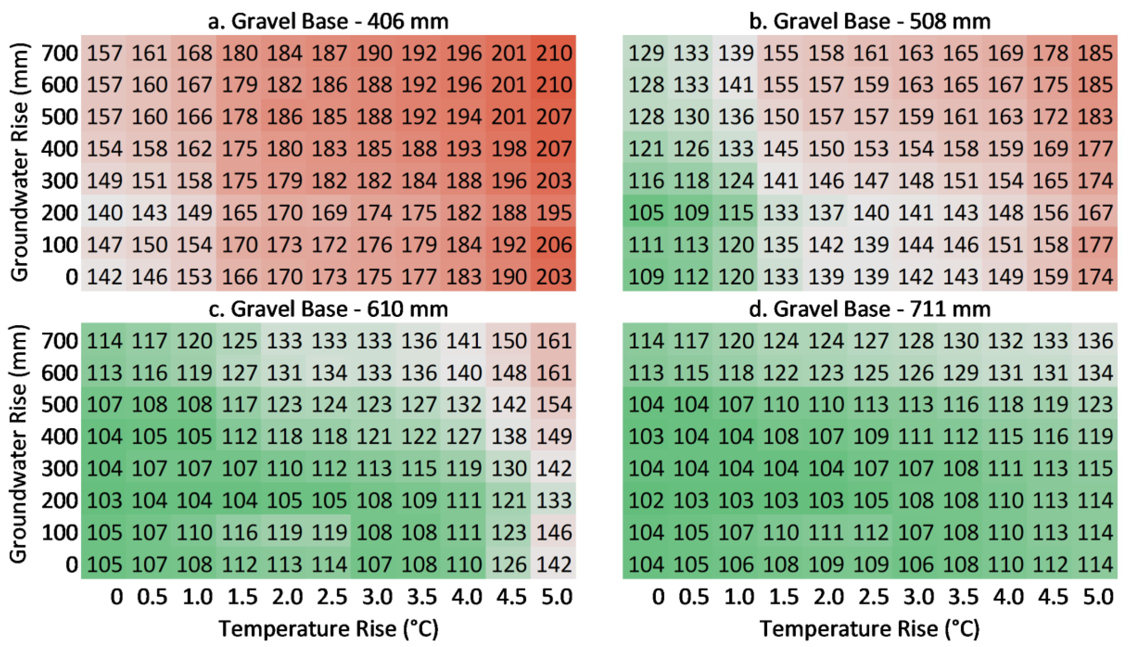
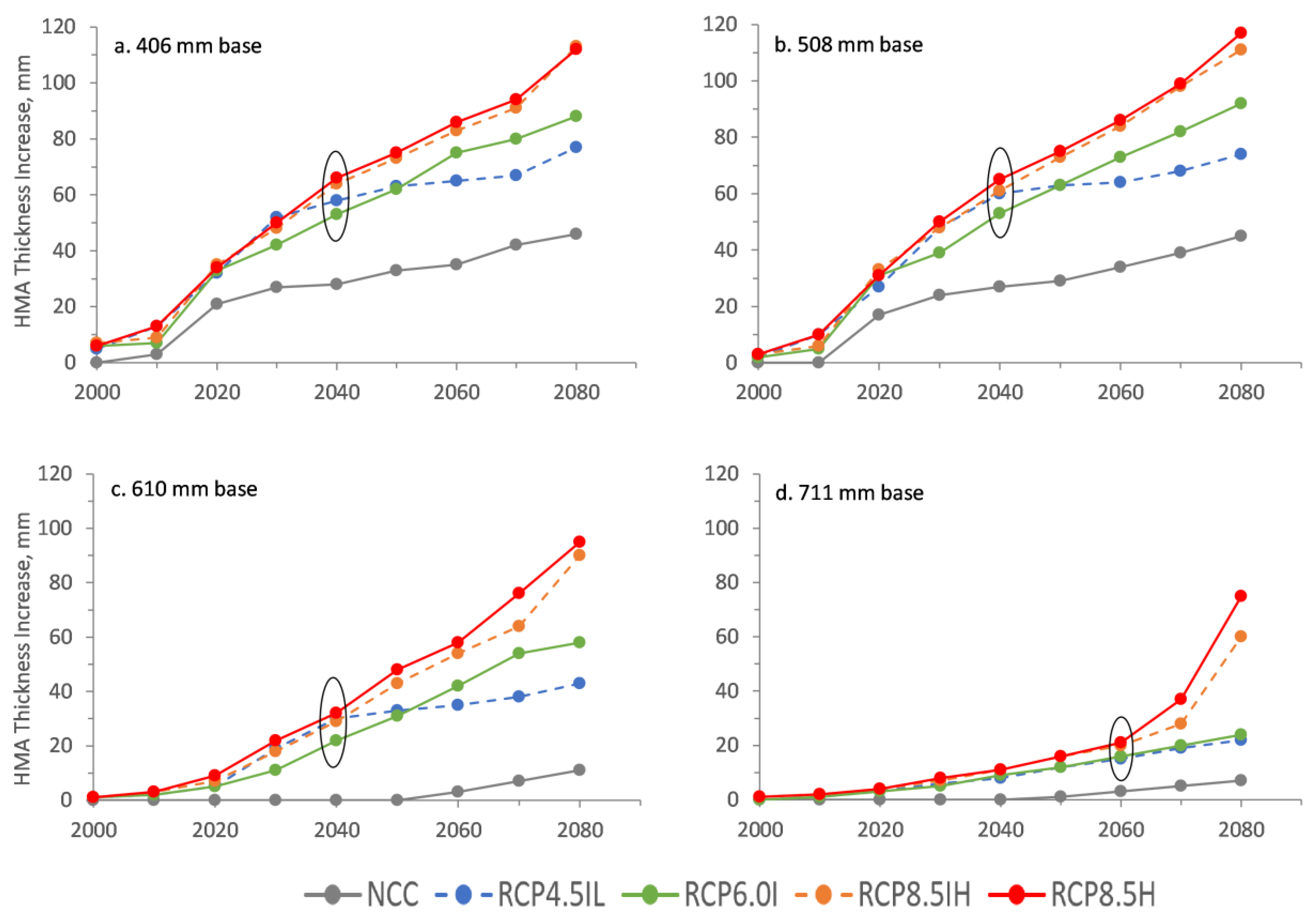
3.1.1. Pavement Climate Sensitivity Catalog (PCSC)

The PCSC is presented in Figure 2 with the O-HMA thickness given in each grid cell for the four gravel-base thicknesses. The PCSC illustrates that the O-HMA thickness decreases with increasing base-layer thickness. The reduction in HMA thickness needed to achieve resiliency with thicker gravel-base layers results in more adaptation capacity through HMA overlays. The O-HMA thickness is more sensitive to temperature increases than groundwater rise, but this is less pronounced with the thicker base layers. For example, the O-HMA thickness required for maximum groundwater rise is sufficient only for a 1 °C temperature rise with 406- and 508-mm base-layer thicknesses. In comparison, the O-HMA thickness for maximum groundwater rise is sufficient for 2.5 °C and 5.0 °C temperature rises with 610- and 711-mm gravel-base layer thicknesses, respectively.
The ratio of O-HMA at a given temperature and groundwater rise to O-HMA with no temperature and groundwater rise (O-HMAT, GW/O-HMA0,0) for each base-layer thickness provides a measure of each structure’s resiliency (Figure 3). Temperature rise from 0 to 3 °C with no groundwater rise for the 508 mm base structure requires an O-HMA thickness increase of 30% increasing to 41% with a corresponding 400 mm groundwater rise. In comparison, for the 610 mm base structure, a 2% O-HMA thickness increase is needed for a 3 °C temperature rise increasing to 15% with a corresponding 400 mm groundwater rise. Increasing the base-layer thickness from 406 to 508 mm does not improve temperature and groundwater rise resiliency. This base thickness provides a large reduction in the O-HMA thickness under current temperatures and groundwater levels, but the benefit is severely reduced with temperature and groundwater rise. Gravel-base thicknesses of 610 and 711 are the most resilient to temperature rise, but this resiliency is reduced with a temperature rise greater than 4.0 °C for the 610-mm base layer and when groundwater moves within 300 mm of the pavement surface for both the 610-mm and 711-mm base-layer thicknesses.
In summary, the bottom-up (asset-based) approach [12,16,17] produced a PCSC in which the sensitivity of four pavement structures with increasing base-layer thicknesses was determined for 70 combinations of incremental temperature and groundwater rise. The following conclusions can be drawn from the PCSC. (1) The PCSC is a useful screening tool in adaptation planning because it illustrates the asset’s sensitivity to incremental environmental change untethered to climate-change scenarios. (2) O-HMA layer thickness (the HMA thickness needed to achieve a minimum of 85% reliability) increases are needed for all four base-layer configurations as temperatures and groundwater rise. (3) Pavement performance is more sensitive to rising temperatures than to rising groundwater for the 406- and 508-mm base layers. Base-layer thicknesses of 610 and 711 mm show improved temperature resiliency. (4) Pavement resiliency is reduced when groundwater moves up in the gravel-base layer. (5) In coastal road infrastructure where both temperature and groundwater are expected to rise, HMA and base-layer thickness increases will be required to maintain pavement reliability. This analysis calculates the O-HMA thickness required for resiliency with different base-layer thicknesses and incremental environmental change. A PCSC could also be designed to evaluate the pavement’s response to loading and changing environmental stressors with improved HMA materials (or other rehabilitation technologies) while keeping the base-layer thickness constant.

3.1.2. Optimal HMA Thickness for Resiliency

The PCSC bottom-up approach illustrates pavement performance changes with incremental temperature and groundwater-rise. This analysis is independent of climate-change scenarios and traffic increases beyond the 20-year design life and the timing of adaptation actions are not considered. Conversely, the scenario-based top-down analysis incorporates projected temperature, groundwater and traffic increases for the 60-year period from 2020 to 2080 enabling the evaluation of stepwise adaptation actions in terms of future performance and cost.
O-HMA thickness increases, i.e., the thickness required to maintain a resilient road, versus time are shown for all the climate change scenarios including a baseline NCC scenario (i.e., traffic increases only) in Figure 4. All the structures need increased HMA thickness over time due to traffic increases and climate change. For the 406 mm base thickness, the mid-century O-HMA increase attributed to climate change (i.e., the difference between the O-HMA increase for the scenarios and the no climate-change increase) ranges from 29 to 33 mm. The increase is less, 11 to 15 mm, and close to typical construction tolerances for the 711 mm base thickness. By the year 2080, the O-HMA increases due to climate change range from 31 to 66 mm and 15 to 68 mm, respectively for the 406- and 711-mm base thicknesses. While the O-HMA thickness increase is less for structures with a thicker base, the relative O-HMA increase with climate change to the traffic-only increases is much higher. This result supports the PCSC finding that a thicker base improves pavement performance with traffic increases and modest climate change, but the resiliency is reduced when the groundwater moves into the base-layer, weakening it, and triggering steep O-HMA thickness increases. The O-HMA thickness divergence among the climate-change scenarios, shown with ovals in Figure 4, typically occurs in 2040 but is delayed until 2060 for the 711 mm base thickness. Prior to divergence, the required increase in HMA thickness is largely the same regardless of the RCP scenario. After divergence, the decision points and adaptation pathways differ by RCP scenario. In practice, mid-to-late-century decisions will be facilitated by increased knowledge about traffic loading, climate change, and pavement material properties.

3.2. Part 2—Adaptation and Costs

3.2.1. Adaptation Pathways and Cost Analysis

Using the results of the pavement performance evaluation, adaptation pathways were created, and life-cycle costs were evaluated to determine the most cost-effective adaptation strategies for this case-study site.

Adaptation Pathways

Thirteen adaptation pathways were created for the NCC, RCP4.5, RCP8.5IH and RCP8.5H scenarios. These pathways were developed using the pavement performance analysis, the O-HMA metric, the four base-layer thicknesses, downscaled climate model output, and estimates of SLR-induced groundwater rise. The RCP8.5IH pathway is used to illustrate the method (Figure 5) with the adaptation pathways’ first action occurring in 2020.
All adaptation pathways begin with the existing gravel base-layer (406 mm gravel) and the calculated O-HMA in 2000 (147 mm) which is slightly greater than the actual HMA thickness at the case-study site (140 mm). The O-HMA thicknesses for 2010 and 2020 are calculated to be 149 mm and 175 mm, respectively, for the RCP8.5IH scenario. The large increase in O-HMA thickness from 2010 to 2020 is due to an increase in recommended minimum pavement life reliability from 85% (ESALs < 1 million) to 90% (ESALs ≥ 1 million) [29]. Each plot (a-d) shows the total O-HMA thickness vs. time for the various adaptation pathways. The incremental overlay thickness is not explicitly shown but is presented as part of the adaptation plan in Section 3.2.3. The colors represent the base-layer thickness. Plot (4a) shows Pathway 1 (P1) in red consisting of a series HMA overlays on top of the existing structure with the timing of each overlay indicated with an X on the pathway. Plot (4b) shows Pathways P1A, P2, P3, and P4. In these pathways, base-layer rehabilitation occurs in 2020. For example, all the pathways begin along the red line and diverge in 2020 to red, orange, green and blue, respectively. In these adaptation pathways, the existing HMA is removed to access and repair and/or increase the thickness of the base layer. In P1A, the base layer is repaired without increasing the thickness. This action is needed if the pavement is experiencing premature failure from pre-existing rutting and/or fatigue cracking. In pathways P2, P3, and P4, the base-layer thickness is increased from 406 mm to 508, 610, and 711 mm, respectively, before repaving with the O-HMA thickness. It is assumed that the old HMA will be recycled in place as 305 mm RSB. Plot (4c) shows pathways P5 through P8 in which the same structural assumptions are made, but rehabilitation is delayed until 2040, i.e., all pathways begin on the red pathway to maintain the O-HMA thickness and diverge to the red, orange, green and blue pathways at 2040. Plot (4d) shows pathways P9 through P12 for which base reconstruction is delayed until 2060.

Adaptation Costs

The average present value of agency and user-delay costs for all pathways and climate-change scenarios are presented in Figure 6. The climate-change scenario influences the pathway cost, but not the pathway ranking in most cases. Regardless of the climate-change scenario, P1 is the least expensive option and, consequently, may be the most desirable; however, there are situations causing premature failure when rehabilitation may be necessary. The two least-costly rehabilitation options for all climate-change scenarios are P11 (base-layer thickness = 610 mm) and P12 (base-layer thickness = 711 mm) with base-thickness increases proposed for year 2060.
If circumstances other than cost drive the rehabilitation timing, the least costly structure is the 610 mm base achieved through pathways P3, P7, and P11. These pathways benefit from an optimal use of on-site RSB that minimizes trucking and user-delay costs. Of these, P11 is the least costly due to a combination of optimal on-site recycling and delayed rehabilitation. If reconstruction is necessary, the most-costly pathway is P1A: reconstruction in 2020 without increasing the base-layer thickness.

3.2.2. Adaptation Strategies

Cumulative probability distributions of present-value total agency and user-delay costs from Monte Carlo simulations are shown for pathways P1, P1A, P3, P7 and P11 for RCP4.5IL, RCP8.5IH, and RCP8.5H in Figure 7. This presentation is useful for decision making because it is a probabilistic approach and reveals uncertainties in the analysis. Costs increase for all pathways with higher emissions/SLR scenarios. The low-cost pathways are consistent across scenarios, but the cost differences among the rehabilitation pathways are less pronounced for the high RCP/SLR scenarios as uncertainty increases. Delaying rehabilitation (P7 and P11) reduces the cost in present-value dollars but also increases cost uncertainty. The least-cost rehabilitation pathway (P11) costs approximately twice the overlay-only pathway (P1) with 85% probability. Increasing the base-layer thickness from 406 mm to 610 mm (P3) saves 20% when compared to constant base-thickness rehabilitation (P1A) under RCP4.5IL and 12% under RCP8.5H. Delaying rehabilitation from 2020 (P3) to 2060 (P11) saves an additional 24% for RCP4.5IL and 10% for RCP8.5H. These results show that there is a large financial benefit to early adaptation using prescribed pavement overlays to avoid the high cost of base-layer rehabilitation. Increased road-surface elevation associated with a thicker pavement structure may result in ancillary costs (not included in the analysis) to modify adjacent properties and connecting roads, but also may delay road surface inundation. Furthermore, this analysis focuses only on HMA and base-layer thickness increases, but if the subgrade is damaged because of a weak pavement structure, the costs of full pavement reconstruction including subgrade repair would be much higher.
Cost is not the only concern when designing a climate-ready coastal road. Some roads will be vulnerable to tidal water and/or groundwater road-surface inundation caused by SLR. At this case-study site, groundwater is projected to regularly inundate the road surface before tidal waters cause overland flooding. The projected groundwater elevation (relative to mean sea level (MSL)) for RCP8.5IH and RCP8.5H is shown with the pavement-surface elevations for each adaptation pathway in Figure 8.
For the RCP8.5IH scenario, groundwater is not projected to be above the existing road-surface elevation (4.33 mm) until 2090. However, the RCP8.5H scenario projections indicate that in 2070, the groundwater will be only 130 mm below the road surface for P1, P1A, P5, and P9, and in 2080, the groundwater will inundate the road surface. Properties at similar elevations served by this coastal road will also flood. Consequently, this case-study site is projected to have flooding problems after 2070 for RCP8.5H (but not the lower RCP scenarios) when following the least expensive (P1) adaptation pathway. Pathways P3, P7 and P11 will delay groundwater inundation of the road surface at RCP8.5H with groundwater projected to be 260 mm and 130 mm below the road-surface elevation in 2070 and 2080, respectively. If the O-HMA is maintained and the costs of premature failure are avoided, P11 is the best choice because road-surface inundation costs and the additional costs of early rehabilitation will both be avoided. Adoption of P11 will also give practitioners the opportunity to re-evaluate adaptation strategies based on new information. Looking beyond 2080, the P3, P7 and P11 road surfaces will be flooded in 2090. This suggests that if the road is still needed to serve properties beyond 2080, P12, an even thicker base, or an elevated road (bridge) will be better than P11. This decision should be made prior to rehabilitation in 2060.

3.2.3. Flexible and Stepwise Adaptation Plan

The previous sections have focused on determining the most cost-effective adaptation pathways for maintaining a resilient coastal evacuation route with projected climate change under NCC and three emissions/SLR scenarios. These pathways are P1, P3, P7, P11, and P12. P1 is the HMA overlay-only option with a 406 mm gravel base. P3, P7 and P11 all require base-layer rehabilitation and thickness increases from 406 to 610 mm but differ when the rehabilitation is done (2020, 2040 or 2060, respectively). P12 involves a base-layer thickness increase from 406 to 711 mm in 2060. An adaptation pathways map and scorecard [32] can be used to develop a flexible and stepwise adaptation plan and are presented in Figure 9. The scorecard gives present value costs for the pathways shown only out to 2080, the end of the pavement management period.
The least costly pathways are P1 and P11, showing that delaying base-layer rehabilitation for as long as possible is cost-effective over the long-term at this case-study site. Regularly assessing the pavement condition, traffic projections, and determining which emissions/SLR scenario is correct at the time of assessment are important factors in choosing the pathways and determining the O-HMA thickness for the prescribe overlays.
An example of how to use the map in Figure 9 is as follows. 1) Begin on pathway P1, the least costly option. If the pavement has pre-existing distresses requiring base-layer rehabilitation, as determined by a field inspection, increase the base-layer to 610 mm (P3) in 2020 and perform the prescribed P3 HMA overlays. If the pavement does not require base-layer rehabilitation continue along P1 and perform the prescribed P1 HMA overlays. (2) Just prior to 2040, the pavement condition, traffic predictions and climate-change scenarios should be re-assessed. If the pavement’s condition is poor, practitioners will rehabilitate the base and increase the base thickness to 610 mm in 2040 (P7). If the pavement’s condition is good, practitioners will continue with P1 overlays until 2060. (3) Just prior to 2060, a similar field, traffic and climate-change assessment is conducted. At this point, SLR-induced groundwater inundation may be occurring in many-low lying areas along the coast and stakeholder options are as follows: (a) follow P1 until the road surface is flooding regularly with groundwater, projected to occur between 2070 and 2080 under RCP8.5H, but later under lower emissions/SLR scenarios; (b) increase the base-layer thickness to 610 mm (P11), delaying possible flooding to between 2080 and 2090; (c) increase the base-layer thickness to 711 mm (P12), delaying flooding until shortly after 2090 under the high emissions/SLR scenario; (d) elevate the roadway, which may or may not be a viable option depending on the flooding exposure of properties served by this road; or (e) abandon the roadway and relocate residents. Decision making at or around 2080 will center around raising the road or road abandonment because further thickening of the base and HMA layers will not adequately address road inundation. The condition of the surrounding land, structures and ecosystems will be important factors in the decision-making process.
The adaptation pathways map shown in Figure 9 does not specify the overlay thicknesses required to achieve the O-HMA. The overlay thicknesses recommended to achieve pavement resiliency at the pavement evaluation site are illustrated in stacked bar graphs for the most cost-effective pathways P1, P3, P7, P11, and P12 under NCC, RCP4.5IL, RCP8.5IH, RCP8.5H in Figure 10. P1A is also included for comparison. P1A is the most-costly pathway, but it reflects a common approach to pavement rehabilitation without considering climate change, i.e., rebuilding the base layer without increasing its thickness.
The recommended HMA overlay thickness (mm) is shown by the number on the bars. The colors represent the year that the overlay should be applied. Large overlay thicknesses marked with a star represent the HMA placed to achieve the O-HMA during repaving after base-layer rehabilitation. The base-layer thickness is not shown in this figure but can be inferred from the pathway name as described in Table 2. This graphical summary readily provides decision makers with recommended HMA overlay thicknesses for chosen adaptation pathways. When there are differences in the incremental overlay thickness between climate-change scenarios, it is recommended that the largest overlay thickness for that pathway and time period be used to avoid the high cost of premature pavement failure. This is a stepwise approach with overlays applied every 10 years, so as we move into the future, uncertainties around which emissions/SLR scenario is correct will decline.
A hypothetical example of how to use this information is as follows: (1) Begin with P1 and RCP8.5H (Plot 8d). In 2020, practitioners apply a 34 mm HMA overlay, followed by 16 mm in 2030, and 16 mm in 2040. (2) Re-evaluate the pavement condition, traffic and climate-change scenarios. At this point, it is determined that the base has been damaged due to pre-existing rutting and fatigue cracking. It is also determined that greenhouse-gas emissions have been reduced sufficiently so that we are now following the RCP4.5IL scenario. (3) Choose P7 in Plot 8b, increase the base layer from 406 mm to 610 mm and repave with 135 mm HMA in 2040. Then apply an HMA overlay of 13 mm in 2050. This should result in pavement resiliency until 2080. If instead, it were determined in 2040 that we are still on the RCP8.5H scenario, practitioners would choose P7 in Plot 8d, repave with 137 mm in 2040, and apply a 16 mm overlay in 2050, a 28 mm overlay in 2060, and a 19 mm overlay in 2080 for pavement resiliency out to about 2085 before the road surface is inundated with rising groundwater. In practice, Figure 9 and Figure 10 are used together to determine the timing and thickness of HMA overlays needed for resiliency.
In summary, after analyzing the pavement’s sensitivity to temperature and groundwater rise using the asset-based PCSC, the top-down (scenario-based) approach was used to determine and evaluate adaptation pathways and costs. Thirteen adaptation pathways were analyzed for performance, cost, and road-surface inundation. O-HMA thickness increases are required across all adaptation pathways. Climate change is a cost multiplier, i.e., the costs of HMA overlays or pavement rehabilitation increase with rising temperatures and groundwater levels. The least-cost adaptation pathway consists of HMA overlays with prescribed HMA overlay thicknesses and an implementation schedule. This pathway is projected to fail, however, between 2070 and 2080 under the high RCP and SLR scenario when groundwater is projected to inundate the road surface.
If pavement structure rehabilitation is needed because of pre-existing distresses or insufficient HMA overlay treatments, unexpected changes in loading and/or climate conditions, or projected road-surface inundation, the existing base-layer thickness should be increased from 406 to at least 610 mm at the case-study site. Increasing the gravel-base layer to 711 mm is slightly more expensive when done after mid-century and may be a viable option if the road is to be used beyond 2080. Pavement-structure rehabilitation with little or no base-layer thickness increase is the most expensive adaptation strategy and should be avoided. The factors controlling the cost differential (in present-value dollars) between rehabilitation pathways are RSB optimization and the timing of the rehabilitation actions. It is best to delay rehabilitation until necessary by implementing prescribed HMA overlays to maintain the O-HMA thickness.
A stepwise and flexible adaptation plan is presented where adaptation actions are taken every 10 years along adaptation pathways from 2020 through 2080. Re-evaluation is recommended every 10 to 20 years to determine (1) the pavement’s condition, (2) changes in projected traffic, and (3) changes in climate projections. Based on the re-evaluation, the adaptation plan can remain on the same pathway or change to another. Early adaptation actions must maximize resiliency, minimize life-cycle costs, and not preclude future actions. The benefits of implementing a prescribed HMA overlay plan include cost minimization and reduction in future uncertainties.

4. Discussion and Conclusions

Many studies have investigated how climate change will affect pavement performance and the cost of pavement maintenance and repair, but few have introduced a method for incorporating climate change into PMS [1,9,10]. This research introduces a hybrid bottom-up/top-down adaptation framework for addressing climate change in pavement design and management by incorporating mechanistic-empirical pavement modeling and climate-change modeling into an existing framework for decision making with uncertainty [32,33]. The approach was demonstrated at a coastal-road pavement evaluation site but can be expanded to inland road infrastructure when planning for climate change. The approach is also well suited for incorporation into PMS [31].
The approach includes both asset-based and scenario-based analyses and was demonstrated at a pavement evaluation site on a regional connector and coastal evacuation route in southeastern NH. The combined effect of temperature and SLR-induced groundwater level increases on pavement life was investigated and a stepwise and flexible adaption plan was developed. The main findings of this case study are:
  • Rising temperatures and SLR-induced rising groundwater will reduce pavement life in coastal roads, but adaptation planning and implementation can reduce the cost of these impacts.
  • Climate-change adaptation for pavements must be based on (1) an understanding of the pavement’s response to the region’s changing climate parameters and (2) an understanding of climate-change projections to determine the timing of the effects.
  • Pavement structural improvements, including HMA overlays and increasing the base-layer thickness result in more resilient pavement with respect to temperature increases and groundwater rise.
  • The adaptation pathway’s cost is sensitive to the emissions/SLR scenario, but the relative-cost ranking was dominated by rehabilitation efficiencies and implementation timing at this case-study site.
  • The optimal HMA thickness is a useful metric for evaluating climate-change adaptation options because it provides practitioners with actionable guidance.
  • Adaptation pathway mapping, as opposed to fixed and robust adaptation actions, provides a stepwise and flexible adaptation plan that maximizes pavement performance and minimizes cost with changing climate conditions over the entire pavement management period.
  • The hybrid adaptation framework for pavement systems can be a model for other systems that have considerable operation and maintenance costs that are projected to increase with climate change.
The hybrid adaptation approach and pathway mapping framework will likely result in different adaptation strategies than either the bottom-up and top-down approaches individually. For example, at this case study site, the results of the PCSC show that the pavement structures with thicker gravel-base layers are more resilient than the structures with less substantial base layers. Likewise, when utilizing only the top-down approach, one or two scenarios are chosen, typically resulting in a robust adaptation plan to achieve resiliency for the chosen worst-case scenario. In isolation, these approaches may result in early reconstruction of the base layer to prevent premature failure. The hybrid framework, while computationally intensive, produces a quasi-continuum of pavement-performance information with incremental climate change. This results in a very different adaptation plan of “just-in-time” actions along an adaptation pathway coupled with life-cycle costs. The resultant adaptation plan provides cost-effective resiliency, the opportunity for reevaluation, and flexibility over time.
The hybrid approach used in this study can be improved by including incremental traffic changes with incremental environmental change when creating PCSCs. Also, investigating a wider range of adaptation options and considering the carbon footprint [69] of each adaptation pathway are both recommended. This analysis investigates the effect of changing layer thicknesses on resiliency. Other options include using a different HMA binder [70] and/or base-layer materials, additives, or geotextiles [41]. A desirable adaptation option would reduce the amount of HMA needed to achieve the desired performance, reduce carbon emissions and reduce costs.
Recommended future work includes incorporating the hybrid climate-change adaptation approach into PMS. Once incorporated, practitioners will be able to (1) identify roads that are vulnerable to changes in climate and more frequent extreme weather events, (2) enhance pavement-life forecasting by including climate change in predictive models, (3) gain increased knowledge of a pavement’s response to loading with changing environmental conditions using a PCSC, (4) identify adaptation pathways, (5) use life-cycle cost analysis with probabilistic present-value cost distributions to compare adaptation pathways, (6) develop a cost-effective adaptation plan that is stepwise and flexible, and (7) re-evaluate and modify the plan, if necessary.
The following research would support incorporating climate change into PMS: Constructing PCSCs for many different climatic regions and for typical pavement structures in various functional classifications of roadways. Developing a simple method for incorporating annual and seasonal changes in environmental parameters and material properties into mechanistic-empirical models. Increasing the number of layers that can be simulated in pavement modeling software which is important when simulating changes in moisture content either from rising groundwater or flooding. More field and laboratory testing is needed to establish relationships between material properties and temperature, moisture content, and degree of saturation.

Author Contributions

Conceptualization, J.F.K., J.M.J., J.E.S. and P.K.; methodology, J.F.K., E.V.D., J.E.S., J.M.J. and P.K.; formal analysis, J.F.K.; writing—original draft preparation, J.F.K.; writing—review and editing, J.M.J., J.E.S.; visualization, J.F.K.; supervision, J.M.J., J.E.S., P.K.; project administration, J.M.J., J.E.S.; funding acquisition, J.E.S., J.M.J.

Funding

This research was funded in part by the University of New Hampshire (UNH) Department of Civil and Environmental Engineering; and the UNH Center for Infrastructure Resilience to Climate (UCIRC). It was also supported by the Infrastructure and Climate Network (ICNet) which was funded by the U.S. National Science Foundation via the RCN-SEES: Engineering Research Collaboratory for Sustainable Infrastructure in a Changing Climate (Grant Number: CBET 1231326).

Acknowledgments

The researchers wish to acknowledge contributions received from the NH Department of Transportation (NHDOT); NH Department of Environmental Services; the NH Coastal Adaptation Workgroup (NH CAW), and the UNH Asphalt Research Group.

Conflicts of Interest

The authors declare no conflict of interest. The funders had no role in the design of the study; in the collection, analyses, or interpretation of data; in the writing of the manuscript, or in the decision to publish the results.

References

  1. Stoner, A.M.K.; Daniel, J.S.; Jacobs, J.M.; Hayhoe, K.; Scott-Fleming, I. Quantifying the Impact of Climate Change on Flexible Pavement Performance and Lifetime in the United States. Transp. Res. Rec. J. Transp. Res. Board 2019, 0361198118821877. [Google Scholar] [CrossRef]
  2. Meyer, M.; Flood, M.; Keller, J.; Lennon, J.; McVoy, G.; Dorney, C.; Leonard, K.; Hyman, R.; Smith, J. Climate Change, Extreme Weather Events, and the Highway System. In Strategic Issues Facing Transportation; Transportation Research Board of the National Academies: Washington, DC, USA, 2014; Volume 2, p. 750. [Google Scholar]
  3. Gudipudi, P.P.; Underwood, B.S.; Zalghout, A. Impact of climate change on pavement structural performance in the United States. Transp. Res. Part D Transp. Environ. 2017, 57, 172–184. [Google Scholar] [CrossRef]
  4. Knott, J.F.; Daniel, J.S.; Jacobs, J.M.; Kirshen, P.; Elshaer, M. Assessing the Effects of Rising Groundwater from Sea-Level Rise on the Service Life of Pavements in Coastal Road Infrastructure. Transp. Res. Rec. J. Transp. Res. Board 2017, 2639. [Google Scholar] [CrossRef]
  5. Daniel, J.S.; Jacobs, J.M.; Miller, H.; Stoner, A.; Crowley, J.; Khalkhalia, M.; Thomas, A. Climate change: Potential impacts on frost—Thaw conditions and seasonal load restriction timing for low-volume roadways. Road Mater. Pavement Des. 2017. [Google Scholar] [CrossRef]
  6. Roshani, A. Road Infrastructure Vulnerability to Groundwater Table Variation Due to Sea Level Rise, Master of Applied Science. Master’s Thesis, Queensland University of Technology, Brisbane, Australia, 2014. [Google Scholar]
  7. Jacobs, J.M.; Culp, M.; Cattaneo, L.; Chinowsky, P.; Choate, A.; DesRoches, S.; Douglass, S.; Miller, R. Transportation. In Impacts, Risks, and Adaptation in the United States: Fourth National Climate Assessment; US Global Change Research Program: Washington, DC, USA, 2018; Volume II, pp. 479–511. [Google Scholar]
  8. Kwakkel, J.H.; Haasnoot, M.; Walker, W.E. Comparing Robust Decision-Making and Dynamic Adaptive Policy Pathways for model-based decision support under deep uncertainty. Environ. Model. Softw. 2016, 86, 168–183. [Google Scholar] [CrossRef] [Green Version]
  9. Chinowsky, P.S.; Price, J.C.; Neumann, J.E. Assessment of climate change adaptation costs for the U.S. road network. Glob. Environ. Chang. 2013, 23, 764–773. [Google Scholar] [CrossRef]
  10. Underwood, B.; Guido, Z.; Gudipudi, P.; Feinberg, Y. Increased Cost to US Pavement Infrastructure from Future Temperature Rise. Nat. Clim. Chang. 2017, 7, 704–707. [Google Scholar] [CrossRef]
  11. Van Aalst, M.K.; Cannon, T.; Burton, I. Community level adaptation to climate change: The potential role of participatory community risk assessment. Glob. Environ. Chang. 2008, 18, 165–179. [Google Scholar] [CrossRef]
  12. Ray, P.A.; Brown, C.M. Confronting Climate Uncertainty in Water Resources Planning and Project Design: The Decision Tree Framework; The World Bank: Washington, DC, USA, 2015. [Google Scholar]
  13. De Bruin, K.; Dellink, R.B.; Ruijs, A.; Bolwidt, L.; van Buuren, A.; Graveland, J.; de Groot, R.S.; Kuikman, P.J.; Reinhard, S.; Roetter, R.P.; et al. Adapting to climate change in The Netherlands: An inventory of climate adaptation options and ranking of alternatives. Clim. Chang. 2009, 95, 23–45. [Google Scholar] [CrossRef]
  14. Smith, J.B.; Vogel, J.M.; Cromwell, J.E. An architecture for government action on adaptation to climate change. An editorial comment. Clim. Chang. 2009, 95, 53–61. [Google Scholar] [CrossRef]
  15. Kwadijk, J.C.J.; Haasnoot, M.; Mulder, J.P.M.; Hoogvliet, M.M.C.; Jeuken, A.B.M.; van der Krogt, R.A.A.; van Oostrom, N.G.C.; Schelfhout, H.A.; van Velzen, E.H.; van Waveren, H.; et al. Using adaptation tipping points to prepare for climate change and sea level rise: A case study in the Netherlands. Wiley Interdiscip. Rev. Clim. Chang. 2010, 1, 729–740. [Google Scholar] [CrossRef]
  16. Taner, M.Ü.; Ray, P.; Brown, C. Robustness-based evaluation of hydropower infrastructure design under climate change. Clim. Risk Manag. 2017, 18, 34–50. [Google Scholar] [CrossRef]
  17. Brown, C.; Ghile, Y.; Laverty, M.; Li, K. Decision scaling: Linking bottom-up vulnerability analysis with climate projections in the water sector. Water Resour. Res. 2012, 48. [Google Scholar] [CrossRef]
  18. Muthadi, N.; Kim, Y. Local calibration of mechanistic-empirical pavement design guide for flexible pavement design. Transp. Res. Rec. J. Transp. Res. Board 2008, 2087, 131–141. [Google Scholar] [CrossRef]
  19. Butler, J.R.A.; Wise, R.M.; Skewes, T.D.; Bohensky, E.L.; Peterson, N.; Suadnya, W.; Yanuartati, Y.; Handayani, T.; Habibi, P.; Puspadi, K.; et al. Integrating Top-Down and Bottom-Up Adaptation Planning to Build Adaptive Capacity: A Structured Learning Approach. Coast. Manag. 2015, 43, 346–364. [Google Scholar] [CrossRef]
  20. Knott, J.F.; Sias, J.E.; Dave, E.V.; Jacobs, J.M. Seasonal and Long-Term Changes to Pavement Life Caused by Rising Temperatures from Climate Change. Transp. Res. Rec. J. Transp. Res. Board 2019, 1–12. [Google Scholar] [CrossRef]
  21. Kwakkel, J.H.; Walker, W.E.; Haasnoot, M. Coping with the Wickedness of Public Policy Problems: Approaches for Decision Making under Deep Uncertainty. J. Water Resour. Plan. Manag. 2016, 142, 01816001. [Google Scholar] [CrossRef] [Green Version]
  22. Wang, W.; Qiu, S.; Wang, S.; Wang, P.; Zhang, J. Investigation of seasonal variations of Beijing pavement condition data using unevenly spaced dynamic panel data model. Int. J. Pavement Eng. 2016. [Google Scholar] [CrossRef]
  23. U.S. Global Change Research Program. Climate Science Special Report: Fourth National Climate Assessment; U.S. Global Change Research Program: Washington, DC, USA, 2017; Volume I, p. 470.
  24. Sweet, W.; Kopp, R.; Weaver, C.; Obeysekera, J.; Horton, R.; Robert Thieler, E.; Zervas, C. Global and Regional Sea Level Rise Scenarios for the United States; NOAA Technical Report NOS CO-OPS 083; NASA: Washington, DC, USA, 2017.
  25. Knott, J.F.; Jacobs, J.; Daniel, J.S.; Kirshen, P. Modeling Groundwater Rise Caused by Sea-Level Rise in Coastal New Hampshire. J. Coast. Res. 2018, 35, 143–157. [Google Scholar] [CrossRef]
  26. De Conto, R.M.; Pollard, D. Contribution of Antarctica to past and future sea-level rise. Nature 2016, 531, 591–597. [Google Scholar] [CrossRef]
  27. Fleming, E.; Payne, J.; Sweet, W.; Craghan, M.; Haines, J.; Hart, J.F.; Stiller, H.; Sutton-Grier, A. Coastal Effects. In Impacts, Risks, and Adaptation in the United States: Fourth National Climate Assessment; US Global Change Research Program: Washington, DC, USA, 2018; Volume II, pp. 322–352. [Google Scholar]
  28. Kumlai, S.; Jitsangiam, P.; Pichayapan, P. The implications of increasing temperature due to climate change for asphalt concrete performance and pavement design. KSCE J. Civ. Eng. 2017, 21, 1222–1234. [Google Scholar] [CrossRef]
  29. Tanquist, B.A. MnPAVE, MNDOT Flexible Pavement Design, Mechanical-Empirical Method. Version 6.2, User’s Guide. Available online: http://www.dot.state.mn.us/app/mnpave/docs/MnPAVE_Users_Guide.pdf (accessed on 1 February 2018).
  30. Tanquist, B.A. Reliability, Damage, and Seasonal Considerations in the MnPAVE Mechanicanistic-Empirical Asphalt Pavement Design Computer Program; Office of Materials, Minnesota Department of Transportation: Saint Paul, MN, USA, 2001. [Google Scholar]
  31. Shahin, M.Y. Pavement Management for Airports, Roads and Parking Lots; Springer: New York, NY, USA, 2005. [Google Scholar]
  32. Haasnoot, M.; Kwakkel, J.H.; Walker, W.E.; ter Maat, J. Dynamic adaptive policy pathways: A method for crafting robust decisions for a deeply uncertain world. Glob. Environ. Chang. 2013, 23, 485–498. [Google Scholar] [CrossRef] [Green Version]
  33. Kwakkel, J.H.; Haasnoot, M.; Walker, W.E. Developing dynamic adaptive policy pathways: A computer-assisted approach for developing adaptive strategies for a deeply uncertain world. Clim. Chang. 2015, 132, 373–386. [Google Scholar] [CrossRef]
  34. Reclamation Downscaled CMIP3 and CMIP5 Climate and Hydrology Projections. Available online: https://gdo-dcp.ucllnl.org/downscaled_cmip_projections/ (accessed on 18 March 2018).
  35. AASHTO. Mechanistic-Empirical Pavement Design Guide (MEPDG), A Manual of Practice, Interim Edition ed; American Association of State Highway and Transportation Officials: Washington, DC, USA, 2008. [Google Scholar]
  36. Huang, Y. KENPAVE—A Computer Package for Pavement Analysis and Design; Pearson: Upper Saddle River, NJ, USA, 2003. [Google Scholar]
  37. Federal Highway Administration. Real Cost Life-Cycle Cost Analysis-User Manual; Version 2.1; Federal Highway Administration: Washington, DC, USA, 2004.
  38. Santos, J.; Ferreira, A. Pavement Design Optimization Considering Costs and Preventive Interventions. J. Transp. Eng. 2012, 137, 911–923. [Google Scholar] [CrossRef]
  39. NHDOT New Hampshire Department of Transportation. Project Viewer. Available online: http://gis.dot.nh.gov/projectviewer/ (accessed on 9 June 2016).
  40. Nemati, R.; Dave, E.V.; Daniel, J.S. Comparative Evaluation of New Hampshire Mixtures on Basis of 1 Laboratory Performance Tests. In Proceedings of the International Society of Asphalt Pavement (ISAP) Conference Proceedings, Fortaleza, Brazil, 19–21 June 2018. [Google Scholar]
  41. Christopher, B.R.; Schwartz, C.; Boudreau, R. Geotechnical Aspects of Pavements, FHWA NHI-05-037. 2006.
  42. Janoo, V. Layer Coefficients for NHDOT Pavement Materials; Special Report 94–30; US Army Corps of Engineers: Washington, DC, USA, 1994; p. 53.
  43. NHDOT Highway Design Manual. Flexible Pavement Analysis; Appendix 7-1; NH Department of Transportation: Concord, NH, USA, 2014; pp. 1–7.
  44. Janoo, V.; Bayer, J.J.; Durell, G.D.; Smith, C.E. Resilient Modulus for New Hampshire Subgrade Soils for Use in Mechanistic AASHTO Design. Specific Report 99–14; US Army Corps of Engineers: Washington, DC, USA.
  45. Federal Highway Administration. Real Cost Life-Cycle Cost Analysis; Version 2.5; Federal Highway Administration: Washington, DC, USA, 2017.
  46. Federal Highway Administration. Long-Term Pavement Performance Computed Parameter: Frost Penetration, Frost Penetration Analysis Results; FHWA-HRT-08-057; Federal Highway Administration: Washington, DC, USA, 2008; Chapter 7.
  47. NH Coastal Lidar Coastal New Hampshire Lidar-2011. Available online: http://lidar.unh.edu2015 (accessed on 15 Augusts, 2015).
  48. Barker, G.; GEOLOGS. New Hampshire Geological Survey; New Hampshire Department of Environmental Services: Concord, NH, USA, 2016.
  49. Department of Environmental Services. One Stop Data and Information. Available online: http://www4.des.state.nh.us/DESOnestop/BasicSearch.aspx (accessed on 15 June 2016).
  50. Federal Highway Administration. LTPP Guide to Asphalt Temperature Prediction and Correction; FHWA-RD-98-085; Federal Highway Administration: Washington, DC, USA, 1998.
  51. Asphalt Institute. Research and Development of the Asphalt Institute’s Thickness Design Manual (MS-1), 9th ed.; Asphalt Institute: Lexington, KY, USA, 1982; p. 204. [Google Scholar]
  52. Shook, J.F.; Finn, F.N.; Witczak, M.W.; Monismith, C.L. Thickness Design of Asphalt Pavements—The Asphalt Institute Method. In Proceedings of the 5th International Conference on the Structural Design of Asphalt Pavements, Delft, The Netherlands, 23–26 August 1982; Volume 1, pp. 17–44. [Google Scholar]
  53. Orr, D.P.; Irwin, L.H. Seasonal Variations of In Situ Materials Properties in New York State—Final Report, CLRP Report No. 06-6. 2006.
  54. Ping, W.V.; Ling, C. Design Highwater Clearances for Highway Pavements; FL/DOT/RMC/BD-543-13; Florida Department of Transportation: Tallahassee, FL, USA, 2008; p. 473.
  55. Elshaer, M. Moisture Dependent Performance of Flexible Pavements. Doctoral Dissertation, University of New Hampshire, Durham, NH, USA, 2017. [Google Scholar]
  56. Witczak, M.W.; Houston, W.N.; Andrei, D. Resilient Modulus as Function of Soil Moisture—A Study of the Expected Changes in Resilient Modulus of the Unbound Layers with Changes in Moisture for 10 LTPP Sites. Development of the 2002 Guide DD-3.35 for the Development of New and Rehabilitated Pavement Structures; NCHRP 1-37 A, Inter Team Technical Report (Seasonal 2); Transportation Research Board: Washington, DC, USA, 2000. [Google Scholar]
  57. Witczak, M.W.; Andrei, D.; Houston, W.N. Resilient Modulus as Function of Soil Moisture—Summary of Predictive Models. Development of the 2002 Guide for the Development of New and Rehabilitated Pavement Structures; NCHRP 1–37 A, Inter Team Technical Report (Seasonal 1); Transportation Research Board: Washington, DC, USA, 2000.
  58. Rockingham Planning Commission. 2040 Long Range Transportation Plan; Rockingham Planning Commission: Exeter, NH, USA, 2017. [Google Scholar]
  59. Seabrook Master Plan Steering Committee. 2011–20 Town of Seabrook Master Plan; Chapter 5: Transportation and Circulation. Available online: http://www.seabrooknh.info/wp-content/uploads/5-FINALTransportation-Chapter-with-Route-One-Corridor-12-6-12-F.pdf (accessed on 3 June 2018).
  60. IPCC. Climate Change 2013: The Physical Science Basis; Contribution of Working Group I to the Fifth Assessment Report of the Intergovernmental Panel on Climate Change; Cambridge University Press: New York, NY, USA, 2013; p. 1535. [Google Scholar]
  61. NHDES. On-Stop Well Inventory. Available online: http://www4.des.state.nh.us/DESOnestop/BasicSearch.aspx2016) (accessed on 16 October 2015).
  62. NHDOT. New Hampshire Department of Transportation—Weighted Average Unit Prices for Projects between 1 July 2017 and 30 June 2018; New Hampshire Department of Transportation: Concord, NH, USA, 2018.
  63. Bozyurt, O.; Tinjum, J.; Son, Y.; Edil, T.; Benson, C. Resilient Modulus of Recycled Asphalt Pavement and Recycled Concrete Aggregate; ASCE Library: Reston, VA, USA, 2012. [Google Scholar]
  64. FHWA. Cost-Based Unit Price: HMA and Aggregate Base. Available online: https://flh.fhwa.dot.gov/resources/design/tools/cfl/.../Cost_Base_Unit_Price.xlsx (accessed on 13 September 2018).
  65. FHWA. Life-Cycle Cost Analysis in Pavement Design—Interim Technical Bulletin; FHWA-SA-98-079; Office of Engineering—Federal Highway Administration: Washington, DC, USA, 1998.
  66. NHDOT. Weighted Average Unit Prices for Projects between 1 April 2016 and 31 March 2017; New Hampshire Department of Transportation: Concord, NH, USA, 2017.
  67. Knott, J.F. Climate Adaptation for Coastal Road Infrastructure in the Northeast. Ph.D. Thesis, University of New Hampshire, Durham, NH, USA, 2019. [Google Scholar]
  68. Office of Management and Budget. OMB Circular Number A-94—Appendix C. Real Treasury Interest Rates from 1979 through 2017. Available online: https://obamawhitehouse.archives.gov/sites/default/files/omb/assets/a94/dischist-2017.pdf (accessed on 15 September 2018).
  69. Thives, L.P.; Ghisi, E. Asphalt mixtures emission and energy consumption: A review. Renew. Sustain. Energy Rev. 2017, 72, 473–484. [Google Scholar] [CrossRef]
  70. Mallick, R.B.; El-Korchi, T. Pavement Engineering Principals and Practice, 2nd ed.; CRC Press, Taylor and Francis Group, LLC: Boca Raton, FL, USA, 2013. [Google Scholar]
Figure 1. Flow chart demonstrating the hybrid bottom-up (asset-based)/top-down (scenario-based) approach to climate-change adaptation for pavements.
Sustainability 11 04382 g001
Figure 2. Pavement Climate Sensitivity Catalog (PCSC) shows the HMA thickness required to achieve 85% reliability (O-HMA) with incremental temperature rise and groundwater rise. The O-HMA color convention is green <140 mm < red. Four gravel-base thicknesses are shown: (a). 406 mm, (b). 508 mm, (c). 610 mm, and (d). 711 mm.
Sustainability 11 04382 g002
Figure 3. Ratio of O-HMAT, GW/O-HMA0,0 for incremental temperature and groundwater rise. The color convention is minimum (green) to maximum (red). Four gravel-base thicknesses are shown: (a). 406 mm, (b). 508 mm, (c). 610 mm, and (d). 711 mm.
Sustainability 11 04382 g003
Figure 4. HMA thickness increases needed to achieve O-HMA thickness for no climate change (NCC) and four climate-change scenarios: RCP4.5IL, RCP6.0I, RCP8.5IH, and RCP8.5H. Four gravel base-layer thicknesses are presented: (a) 406 mm, (b) 508 mm, (c) 610 mm and (d) 711 mm.
Sustainability 11 04382 g004
Figure 5. Adaptation pathways (a) P1, (b) P1A to P4, (c) P5 to P8, and (d) P9 to P12 shown as the calculated O-HMA thickness vs. time for RCP8.5IH. The colors represent the base-layer thickness as follows: red-406 mm (P1, P1A, P5, P9), orange-508 mm (P2, P6, P10), green-610 mm (P3, P7, P11), blue-711 mm (P4, P8, P12). Colored Xs represent the HMA overlays for individual pathways. Black Xs represent overlays in all pathways within each subplot. Bull’s eyes represent base-layer rehabilitation with colors corresponding to the final base-layer thickness.
Sustainability 11 04382 g005
Figure 6. Projected average agency and user costs in present value dollars for 13 adaptation pathways with NCC, RCP4.5IL, RCP8.5IH, and RCP8.5H scenarios. The solid bars represent the average agency cost and the hollow bars represent the user-delay costs. The pathways are given along the horizontal axis and are described in Table 2.
Sustainability 11 04382 g006
Figure 7. Probability distributions for total costs associated with pathways P1, P1A, P3, P7, and P11 for RCP4.5IL, RCP8.5IH, and RCP8.5H.
Sustainability 11 04382 g007
Figure 8. Pavement surface elevation at the pavement evaluation site relative to the mean sea level (MSL) for the 13 adaptation pathways is shown by the bars for each decade from 2020 to 2080. The inverted triangle marks the projected groundwater-surface elevation for the indicated year and RCP/SLR scenario. The projected groundwater elevation is shown for years 2070, 2080, and 2090 for the RCP8.5H scenario and 2090 for the RCP8.5IH scenario.
Sustainability 11 04382 g008
Figure 9. Adaptation pathways map showing the most cost-effective adaptation pathways and the cost scorecard. The timing of HMA overlays is illustrated with X and tipping points, where a transfer to a different pathway may occur, are shown with a bull’s eye symbol. Solid lines represent viable pavement structures for all scenarios and dashed lines represent viable pavement structures for some, but not all scenarios. PV is present value. (Modified from Haasnoot et al., 2013) [32].
Sustainability 11 04382 g009
Figure 10. Cumulative HMA overlays required to maintain O-HMA thicknesses for select pathways. Colors represent the timing of the overlay. Overlay thickness in mm is indicated by numbers. Black stars mark the HMA thickness to be placed after base-layer thickening. Each chart represents: (a) NCC, (b) RCP4.5IL, (c) RCP8.5IH, and (d) RCP8.5H.
Sustainability 11 04382 g010
Table 1. Projected temperature (Temp.) rise, groundwater (GW) depth and traffic at Route 286 in coastal New Hampshire for three emissions scenarios: RCP4.5, RCP6.0, and RCP8.5 and four SLR scenarios: Intermediate Low (IL), Intermediate (I), Intermediate High (IH) and High (H); F = Pavement Surface Flooded.
YearRCP4.5 Intermediate LowRCP6.0 IntermediateRCP8.5 Intermediate HighRCP8.5 HighTraffic (ESALs/106)
Temp. Rise (°C)GW Depth (mm)Temp. Rise (°C)GW Depth (mm)Temp. Rise (°C)GW Depth (mm)Temp. Rise (°C)GW Depth (mm)
20000.37000.47000.47000.47000.944
20100.76720.76630.86440.86300.944
20201.16441.06121.25931.25611.000
20301.56121.35651.75141.74821.061
20401.85841.75192.24592.23801.124
20502.15522.04632.73712.72731.191
20602.35242.33983.42733.41501.263
20702.55122.73434.01874.0161.337
20802.74943.02794.8864.8F1.416
Table 2. Description of adaptation pathways for analysis.
PathwayInitial Base Thickness (mm)Base Rehab.?Year of Base Rehab.New Base-Thickness (mm)Description
P1406No--O-HMA overlays only
P1A406Yes2020406Remove HMA, repair base, repave
P2406Yes2020508Recycle HMA, add 102 mm base, repave
P3406Yes2020610Recycle HMA, add 204 mm base, repave
P4406Yes2020711Recycle HMA, add 305 mm base, repave
P5406Yes2040406Remove HMA, repair base, repave
P6406Yes2040508Recycle HMA, add 102 mm base, repave
P7406Yes2040610Recycle HMA, add 204 mm base, repave
P8406Yes2040711Recycle HMA, add 305 mm base, repave
P9406Yes2060406Remove HMA, repair base, repave
P10406Yes2060508Recycle HMA, add 102 mm base, repave
P11406Yes2060610Recycle HMA, add 204 mm base, repave
P12406Yes2060711Recycle HMA, add 305 mm base, repave

