Measuring Cross-Border Road Accessibility in the European Union

Abstract

Border regions are in the forefront of geographical cohesion of the European Union but often lag behind more central areas on development and connectivity. As transport infrastructure—or rather the lack of it—plays a primary role in this, specific policy measures to improve the quality of road connections and address the overall issues of geographic isolation are often necessary. The methodology presented here provides a set of indicators and tools that allow policy makers to measure accessibility and connectivity of border regions, identify areas where transport infrastructure may be lacking, and prioritize potential investments based on specific policy-relevant criteria. The approach uses very detailed spatially disaggregate data covering EU28 plus Norway and Switzerland at grid level (1 km by 1 km), as well as the complete road network. This level of resolution allows many of the specificities of the areas covered to be taken into account.

1. Introduction

This paper presents a methodology to measure and evaluate the accessibility of border regions, focusing on the internal border of the European Union (EU). The approach addresses three main research questions: How to measure accessibility; how cross-border accessibility compares to accessibility within the national territory; and how accessibility analysis can be employed for policy analysis. The main target is to assess the road network of border regions across the EU. By conducting the analysis at fine resolution and for the complete road network, it is possible to identify, with relative precision, well performing areas and parts that may require infrastructure investments. Most relevant studies so far have been focusing on specific, geographically-limited, cases aggregated at a relatively coarse spatial level—such as regional or municipal.

The EU has 38 internal land border regions, which represent almost 13% of its total population. However, border regions are—at large—more isolated than the rest of the Member State they form part of. On one hand, since most EU Member States have developed their infrastructure and regional policy with a centralized state in mind, their peripheries have not generally received as much investment as their cores, usually their most central areas. In addition, the lack of investment has led to the acceleration of the movements from the periphery to the core, leading to a vicious cycle of further reduced investments in peripheral areas of decreasing importance in population and economic terms. On the other hand, border regions face geographic, historical, cultural, and linguistic barriers that limit their opportunities for interactions with their cross-border counterparts which— in most cases —are also isolated within their own national context. These two trends, the internal and the cross-border isolation, mean that a significant part of the EU population has limited access to opportunities, even though they may no longer be considered as “frontier” zones within the European Union.

The European Commission adopted the Communication ‘Boosting Growth and Cohesion in EU Border Regions’ (European Commission, 2017) [1] to address the difficulties that border regions face, and propose a series of concrete actions to improve cross-border collaboration. The Communication highlights ways in which the EU and its Member States can reduce the complexity, length, and costs of cross-border interaction, and promote the pooling of services along internal borders. The positive effects of reducing cross-border obstacles can contribute both to the socio-economic development and the integration of border areas. The European Commission has a major role in this process by proposing legislation or funding mechanisms, or by supporting Member States and regions to better understand the challenges and develop operative arrangements, notably by promoting information sharing and showcasing successful practices.

Transport infrastructure plays a critical role in the connections of border areas and can influence regional, urban, or local development. The Trans-European Network for Transport (TEN-T) is of the utmost importance for the improvement of transport services and cohesion in Europe, but it is not sufficient to cover the connectivity deficits of border regions. Border regions are literally in the forefront of geographical cohesion of the EU member states, but often appear to be poorly developed and heterogeneous in terms of transport infrastructure. In fact, physical access was the third most cited obstacle (following legal/administrative barriers and language) regarding border regions in a relevant public consultation of the European Commission [2]. The lack of transport infrastructure can either be an issue of natural obstacles, such as rivers or mountains, or an issue of capacity when the existing infrastructure does not cover the high demand because of high interaction levels between the areas sharing a common border.

One of the main challenges regarding networks’ integration for the European Commission has been to address relevant inefficiencies by contributing to the development of necessary transport infrastructure. As a result, it is important to identify areas in need, or better, to classify and benchmark border regions according to accessibility and road infrastructure.

The structure of the paper is the following: Section 2 discusses the theoretical background of accessibility analysis and its relevance to border regions. Section 3 presents the data used, while Section 4 discusses the three main accessibility indicators applied. Section 5 presents the numerical results, which are further discussed in Section 6. Finally, the conclusions are presented in Section 7.

2. Accessibility Analysis and Border Regions

Accessibility is a well-known concept that is increasingly used in transport and land use planning. Improving accessibility has become a main priority for policy makers at national, regional, and local level (Christidis et al. 2012) [3]. The international dimension of accessibility is, however, not widely studied. Most studies address the national context (Stepniak et al. 2013) [4]. The need to explore—specifically the case of border regions—is raised by Salas-Olmedo et al. (2015) [5], especially in the context of identifying proxies to explain the effect of borders as obstacles in trade and collaboration. Rietveld (2012) [6] estimates a substantial border effect responsible for a 30–70% reduction in trade, depending on transport mode and infrastructure. Rotoli et al. (2014) [7] link accessibility to consumer surplus and identify a significant positive correlation at regional level, especially concerning peripheral zones.

The reasons why border regions lag behind in terms of transport infrastructure may have to do with their nature; often they lack the critical mass to justify transport investments (Condeço-Melhorado et al. 2018) [8] or are managed by different authorities which do not always cooperate efficiently. López et al. (2009) [9] refer to the issue of ‘missing networks’, the existence of which—according to Maggi et al. (1992) [10]—can be attributed to the fact that for transport development, each country tries to address their problem, ignoring the potentials of cooperation and without attempting to coordinate actions. Halás et al. (2014) [11] carry out an exhaustive analysis of accessibility of Czech regions and witness a strong influence of both physical and administrative barriers. In general, zones near border areas suffer from a deformation of their potential hinterlands, an indication of a disadvantage compared to central zones. Zhang et al. (2019) [12] explore the operational characteristics of road networks at various scales and contexts. They identify small-world network characteristics in both urban and rural areas, but the differences in scale lead to rural networks being less efficient. In addition, they confirm the existence of the cross-border effect, at least with regard to freight transport.

The relationship between accessibility and development has been investigated in several cases, especially in the context of assessing major infrastructure investments. There are many definitions and indicators of accessibility, addressing different aspects of the topic and covering specific assessment needs. Geurs et al. (2004) [13] and Geurs et al. (2004) [14] provide a thorough review of accessibility indicators based on multiple criteria, taking into account different perspectives. They classify indicators in four main categories: Infrastructure-based, location-based, person-based, and utility-based indicators. The different categories aim to cover distinct areas of planning or assessment, and use information at different levels of detail. The choice of the most suitable indicator depends on a combination of factors, including data availability and type of analysis required. Selecting a more informative and detailed indicator is not necessarily the best choice because it might be difficult to obtain the required data. Lopez et al. (2008) [15] use four different accessibility indicators to measure how cohesion has changed over the years in Spain. Each indicator corresponds to different approaches, focusing on either the location or the infrastructure, in combination with different measurement formulations. The population potential indicator or the daily accessibility indicator measure reachable population or activities, while the location indicator or network efficiency indicator use the population of destinations as weighting of travel cost measures.

The assessment of network infrastructure and accessibility at regional scale produces relatively rough estimates, suitable for analyses at country level or for analysing the impacts of large national or international projects. Gutierrez et al. (2011) [16] used the market potential (an indicator based on the structure of potential accessibility indicators, which will be presented in more detail later in this section) to measure the impact of TEN-T projects at province level (NUTS 3 level following the European regional classification system Nomenclature of territorial units for statistics); they concluded that “the construction of border sections is not very efficient due to the border effect (they produce a lower increase in market potential), though they generate many spill-overs. Internal sections, by contrast, are more efficient, producing more internal benefits but comparatively fewer spill-overs.”

Rotoli et al. (2015) [17] followed a Data Envelopment Analysis approach to estimate the benefits at regional level from increased accessibility and suggested a positive correlation. Rokicki et al. (2018) [18] identified a weak—but positive—correlation between accessibility and regional employment. Arvemo and Gråsjö (2018) [19] explored the importance of cross-border activities for border regions in Sweden by dividing them into three categories, depending on the population density on each side of the national border. The largest positive effect in terms of economic development can be found for municipalities belonging to sparsely populated regions bordering a densely populated region. Municipalities in densely populated regions bordering a densely populated region have a marginally lower advantage. The third combination, municipalities in sparsely populated areas bordering rural areas, appears to be limited by the lack of opportunities on either side of the border.

There are numerous formulations of accessibility indicators that can highlight different attributes. In any case, for the identification of the appropriate measure, it is important to understand the attributes of the case study area and the priorities of the analysis, taking into account data availability. The formulation of the accessibility indicator and the parameters used in its operationalization have also been widely explored, without—however—reaching a definitive conclusion. Condeço-Melhorado et al. (2016) [20] study the issue of internal distances in order to address the distortion created when analyzing highly aggregated spatial units. Grid-based measures appear to introduce smaller errors than region-based ones. In a subsequent application, Condeço-Melhorado et al. (2017) [21] decompose the infrastructure and population elements of potential accessibility and explore their respective roles. Stępniak et al. (2018) [4] carry out a detailed comparison of the distance decay functions used in accessibility indicators and their influence in the interpretability of the results. Martens and di Ciommo (2017) [22] propose that changes in accessibility should be incorporated in Cost-Benefit Analysis (CBA) in order to address equity and distributional effects, but observe that directly replacing travel time savings with accessibility gains is not sufficient to address the equity aspects. Thomopoulos et al. (2009) [23] review the principles and alternative approaches of CBA and Multi-Criteria Analysis (MCA) methods, and propose a hierarchical process that allows spatial equity and cohesion aspects to be taken into account. The relative weights of strictly economic criteria as opposed to those of environmental or equity concerns are still under discussion and depend on the specific application. Nahmias–Biran and Shiftan (2016) [24] propose a Subjective Value of Accessibility Gains approach, a hybrid of CBA and MCA that uses accessibility indicators instead of the more common Value of Time (VoT). Lucas et al. (2016) [25] adopt egalitarianism and sufficientarianism theories to evaluate the equity and accessibility aspects of transport policy.

3. Data

The main issue addressed in this study is the assessment of the quality of cross-border road infrastructure using suitable indicators at a level of spatial resolution that allows the physical interpretation of the results. A consistent set of indicators at EU level can assist policy makers in identifying areas for improvement and future investment, as long as these indicators rely on easily measureable data and are expressed in units that have a direct correspondence to policy relevant variables. For this purpose, the following datasets have been combined:

(1)

Population distribution map at 1 km by 1k m grid for the areas defined as border zones, based on the following European Commission sources: Eurostat, Joint Research Centre and Directorate General for Regional and Urban Policy (DG REGIO). The fine resolution used has the advantage of avoiding demarcation problems associated with the selection of nodes or use of nodes as point representations of regions (Bruinsma and Rietveld, 1998) [26]. At this level of granulation, the distortion caused by the internal distances of the spatial unit used in minimized. Population distribution maps are readily available and visualizing accessibility at this level is probably the optimal way to map equity issues. Population has been selected as the attraction/weighting factor for the operationalization of the indicators, since it is readily available and is a good proxy for most economic and social interactions. This is in line with [4], where the majority of accessibility studies surveyed also used population as the attraction factor. A notable exception is [13], where jobs were used as an attraction factor which—as a result—allowed a deeper analysis of employment issues to be feasible. Furthermore, in research by Gutierrez and Monzón (1998) [27], instead of weighting the ratio of travel times by population, it is weighted by the incomes at the economic centres of the destinations. Economic activity might be more representative of the attractiveness of a settlement as a destination than population. However, it is very difficult to obtain reliable data of economic activity, especially at the scale required, while population is directly related to the attractiveness of a destination.

(2)

Map of settlements with population of over 5000 inhabitants in Europe, based on the following European Commission sources: Eurostat, Joint Research Centre and DG REGIO. Depending on the formulation of the accessibility indicator used, the attraction variable can either consist of individual grid-based values or aggregates of grid cells that correspond to settlements.

(3)

Detailed transport network at European level provided by TomTom [28]: A road network that includes (practically) the full European road network. This provides the double benefit of full coverage of route options and full connectivity with the grid-based map of population. As a result, the distances and travel times that can be calculated are as realistic as possible. Travel times are based on the calculation of the shortest path using speed information included in the TomTom data for each link that is part of the shortest path. The points of departure are the centroids of the inhabited 1 km by 1 km grid cells within a 25 km buffer of national terrestrial borders, and the points of arrival are the centroids of settlements with population larger than 5000 inhabitants. More specifically, travel times between the nodes of the road network that are closest to the origin and destination points are calculated.

4. Measurement of Accessibility

Different formulations of accessibility indicators tend to address specific dimensions of the relationship of a point in space with its surroundings. For example, using the classification of Geurs and van Wee (2004) [13] and Geurs and Ritsema van Eck (2004) [14], infrastructure-based indicators consider the quality of service (travel time, congestion time etc.) but ignore issues related to activities in the destinations. On the other hand, location-based accessibility measures include both a measure of opportunities in the destination zone and a measure of distance or cost of travel between the origin and destination zones. Furthermore, potential accessibility indicators include a cost sensitivity parameter that aims to capture spatial travel behavior. Location-based accessibility indicators are the most relevant to the purposes of this study as they can analyze performance of road networks, including a measure of importance of destinations.

The specific policy question analyzed here—i.e., the role of road infrastructure in border regions—can be addressed using three different types of operationalization of accessibility indicators that quantify three underlying aspects relevant to the spatial relationships of each border region:

(1)

Location indicator as a measure of a border region’s connectivity;

(2)

Potential indicator as a measure of a region’s access to opportunities; and

(3)

Network efficiency as a measure of the quality of a region’s road connections.

Each indicator on its own allows a comparison between the national and international accessibility of each zone, but the pairwise combinations of the three indicators permit further insights into the reasons of the observed situation and—in particular —the evaluation of the potential impacts of improvements in the road network on cross-border accessibility. The attraction factor used in all three accessibility indicators is population.

In general, the scale of application—Europe as a whole analyzed at grid level, in the specific case—dictates the choice of indicators, variables, and methods. The combination of population data at grid level, data regarding settlements, and a very detailed road network makes this analysis unique. At the same time, processing data of such detail and size is quite challenging.

4.1. Location Indicator

The first indicator calculated is the location indicator, which measures travel time weighted by the population of destinations. It is given by the following formula (Gutierrez et al, 1996) [16]:

$$L{I}_i=\frac{{{\displaystyle \sum }}_{j=1}^n{t}_{ij}{P}_j}{{{\displaystyle \sum }}_{j=1}^n{P}_j}$$

(1)

This indicator should be interpreted from a locational perspective as it represents the travel time between a location and a number of points of interest (Gutierrez, 2001) [29], where:

t_ij the travel time from cell i to destination zone (settlement) j;

P_j the population of destination zone j; and

n the number of points of interest (destination zones or settlements j) to be taken into account in the calculation.

The indicator is expressed in time units, and its physical interpretation is how long on average it takes to drive from each cell to the main activities. Travel times are calculated separately for each destination.

4.2. Potential Accessibility

The second indicator used is potential accessibility, which is classified as a gravity-based indicator, considering the way it incorporates travel time. Travel time is raised to the power of α in order to control the importance of the role of distance or time between origin and destination. Values larger than 1 (i.e., a higher decay function parameter) increase the importance of relations over short distances (Gutierrez, 2001) [29].

$$P{A}_i=\frac{{{\displaystyle \sum }}_{j=1}^n{P}_j}{{{\displaystyle \sum }}_{j=1}^n{t}_{ij}{}^a}$$

(2)

where:

t_ij the travel time from cell i to destination zone (settlement) j;

P_j the population of destination zone j;

n the number of points of interest (destination zones or settlements j) to be taken into account in the calculation; and

a is a parameter to control the decay function.

This indicator should be interpreted from an economic perspective, as it measures the economic potential of each place considered and the changes to be caused by new infrastructure (Gutierrez, 2001) [29]. The formulation used here follows Condeço-Melhorado et al. (2017) [21] and Rotoli et al. (2015) [22], and applies a parameter a = 1, which corresponds to a linear decay function. While other, higher, values can be considered, the spatial delimitation of the area of interest in this specific application makes this selection non-critical (as Stępniak & Rosik, 2018 [4] also suggest). We use a radius of 75 km, which results in the mean of the travel distances and travel times in the border areas analyzed to be 68 km and slightly below 1 h (55 min), respectively. This effectively transposes the objective to that of estimating a daily accessibility indicator. Martínez and Viegas (2013) [30] estimate the daily activity trip duration threshold to be 60 min. All destinations within the area of interest are considered as of equal importance. The value of the resulting indicator for each cell is proportional to the sum of population accessible from the cell per unit of travel time (e.g., hour).

4.3. Network Efficiency

Network efficiency indicators were initially proposed by Gutierrez and Monzón (1998) [27] as an elaboration of the ‘route factor’ used to measure the sinuosity of individual links. The rationale is to reduce reliance on geographic location—or “neutralize the impact of the geographic location”—and assess transport infrastructure needs or potentials of a region. The network efficiency indicator considers accessibility on the existing network and accessibility on an ideal network in order to indicate the potential of improvement of the network.

The network efficiency indicator NER, which is reported in the results of this study, is the reverse of Network Efficiency (NE), which is calculated according to the following formula:

$$N{E}_i=\frac{{{\displaystyle \sum }}_{j=1}^n\frac{t_{ij}}{t_{ij}^{\prime }}{P}_j}{{{\displaystyle \sum }}_{j=1}^n{P}_j}$$

(3)

I.e., NER is given by the following formula:

$$NE{R}_i=\frac{1}{N{E}_i}$$

(4)

Where:

t_ij is the travel time on the network from origin zone i to destination zone j;

t′_ij is the time needed to cover the straight line distance between origin zone i and destination zone j when travelling with a constant speed of 120 km/h;

P_j is the population of destination zone j; and

n is the total number of destination zones to be considered, in this specific case n = 5.

As t_ij is the ideal travel time, NE_i will tend towards 1 as accessibility improves and will increase as accessibility reduces. By reversing network efficiency, the NER_i indicator obtains values between 0 and 1, so that values reaching 1 indicate high network efficiency while values reaching 0 low.

The network efficiency indicator takes into account attributes of the network by including a variable representing ideal travel time. The ideal travel time incorporates issues regarding both road length and speed, as it refers to travel time for a straight line distance between two points under a maximum speed. As a result, the speed has to do with the type of road and the length with the design that may be influenced by several factors, including the geomorphology.

Network efficiency is a suitable indicator to assess and benchmark road infrastructure of border regions. In addition to performance of the network (travel time) and attractiveness of potential destinations (population), it includes a parameter representing ideal performance of the network. As a result, the indicator focuses on the characteristics of the network, remains unaffected by the physical distance between origin and destination, and uses population to weight travel time.

5. Results

National and international accessibility indicators are calculated separately for each couple of countries sharing borders. For each origin zone (grid cell), national accessibility is calculated considering the five most populated settlements in the same country within a radius of 75 km, and international accessibility is calculated considering the five most populated settlements in the neighbouring country within a radius of 75 km. Both the number of five settlements and the 75 km threshold were selected empirically as a sufficient approximation of the policy objectives that define this study. Using fewer than five settlements may lead to unstable results that over-rely on specific settlements, while using more increases computation time without any meaningful change in the results. The consideration of 10 (five national and five cross-border) destinations from each grid cell is absolutely sufficient to capture the attributes of the network.

Since a constant radius of 75 km around each cell is used, the cells farthest from the border have potentially higher accessibility to population in their national territory, rather than to population in the neighbouring one. The radius of 75 km has been determined to take into account settlements within relative proximity. The means of the travel distances and travel times to the selected settlements are 68 km and slightly below 1 h (55 min), respectively. Measuring accessibility at fine resolution level makes it possible to capture, with high precision, the potential destinations of interest. As a result, reality is represented better in comparison to considering only major cities.

The location indicator measures travel time weighted by the population of the destination. In this case, population represents the attractiveness of a zone and is used to weight travel time, while accessibility is measured in terms of travel time—i.e., the smaller the location indicator, the higher the accessibility. On the other hand, the potential accessibility indicator measures the number of accessible population considering travel time. Adopting a gravity approach, the population is used as a measure of attractiveness, the intensity of which decreases with distance, travel cost, or travel time. Hence, in this case, the larger the potential accessibility indicator, the higher the accessibility. Finally, the network efficiency indicator has a structure similar to the location indicator, but takes the ideal travel time also into account. Hence, accessibility is relative to ideal travel time and improves as travel time approaches the ideal one.

5.1. Location Indicator

The median of the location indicator at national level is 49 min (i.e., for half of the cells more than 49 min are needed to reach the main activities), while the median on the international side rises to 59 min. As another comparison measure, the median of the ratio between the international and national side is 1.2—i.e., 20% longer travel time on the international side than on the national side. It is worthwhile to note that a large number of cells have a ratio lower than 1, meaning that the travel time to activities in the neighbouring country is lower than in the country they belong to. On the other hand, while at national level most activities can be reached within 1.5 h, the distribution at international level has a longer tail, with a larger share of cells over the 1.5 h mark.

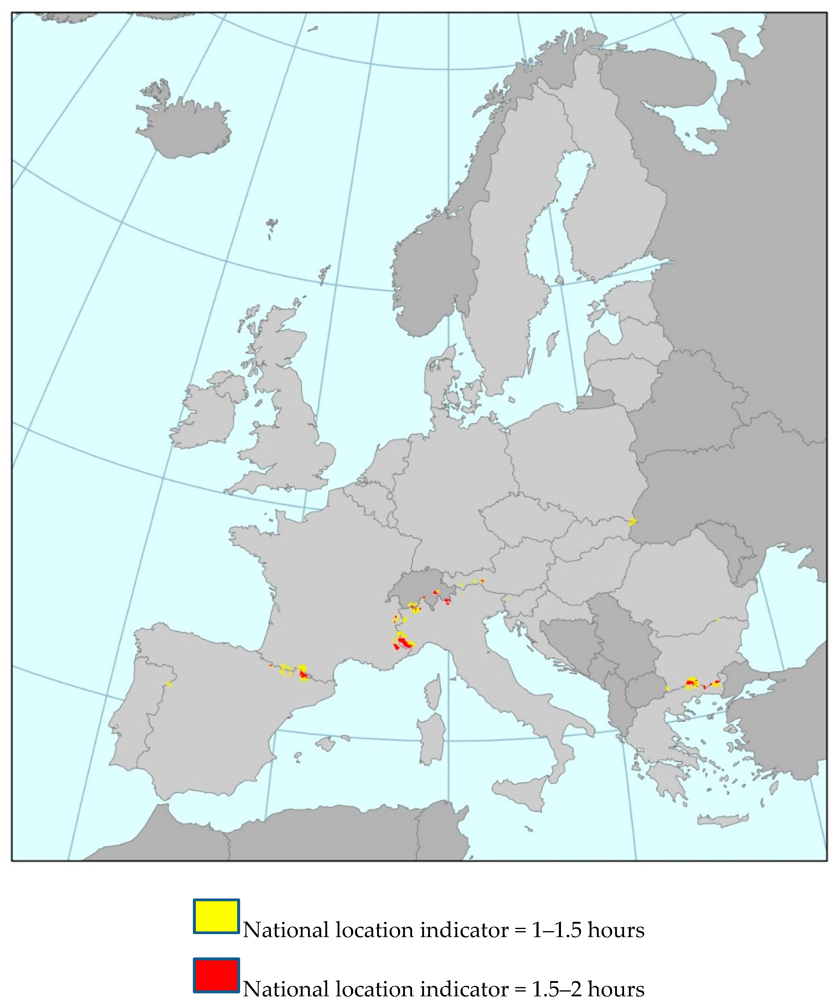
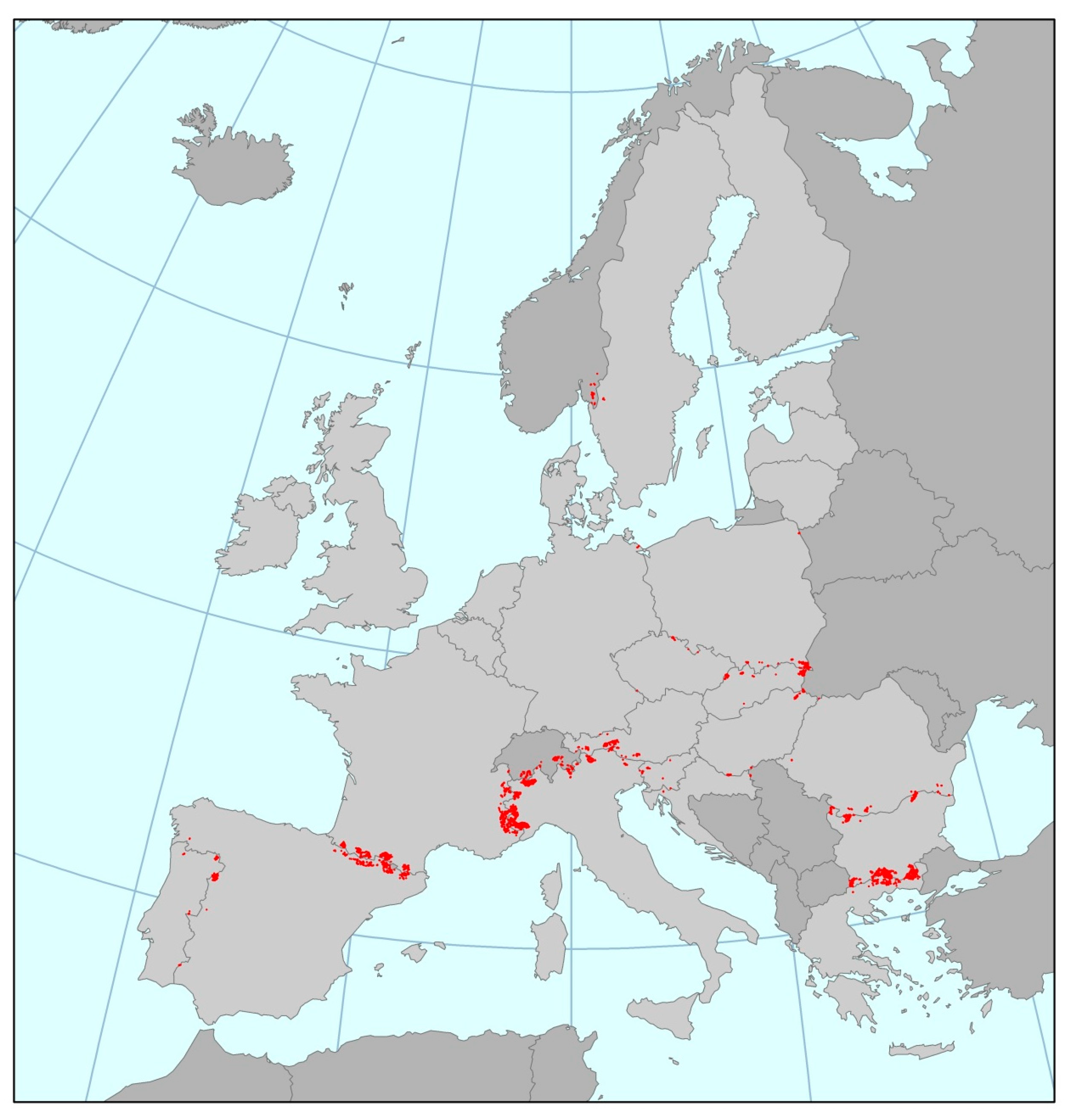
As an example, the zones with an international location indicator higher than 2 h can be seen in Figure 1, with a comparison of the national location indicator for the same cells. Cells with high values on both sides of the border (in red) are probably isolated because of the morphology of the area, such as the Alps, the Pyrenees, and the Rodopi ranges. The points on the Bulgarian-Romanian border are the result of the lack of river crossings over the Danube.

The location indicator can provide useful information for the identification of isolated areas and for the comparison between the international and the national side. As an indicator of isolation, the direct comparison of the value of the indicator, regardless of whether it addresses the national or the international side, can provide an objective assessment of the situation. In the example of Figure 1, it is clear that all zones in red are highly isolated, since they are at least 2 h away from the main activities in either their own country or the neighbouring one. The areas in yellow are better connected on the national side (1–1.5 h) than on the international one (more than 2 h), but still, the role of physical geography obstacles are visible.

5.2. Potential Accessibility Indicator

For the national part, the mean Potential Indicator is 923 thousand persons per hour, with the median being 416 thousand persons per hour (the long tail of the distribution causes high skewness). For the international part, the figures are much lower, with a mean of 379 thousand persons per hour and a median of 191 thousand persons per hour. From the analysis of the results, a large number of cells have low values for both national and international potential accessibility. Those cells probably correspond to rather isolated areas close to the border. Also, two other distinct groups can be identified: The majority corresponds to cells with high values for national and low values for international (zones farther from the border with no significant levels of population in the neighbouring country), but an interesting group from the policy perspective consists of the zones with low values for national and high values for international Potential Accessibility.

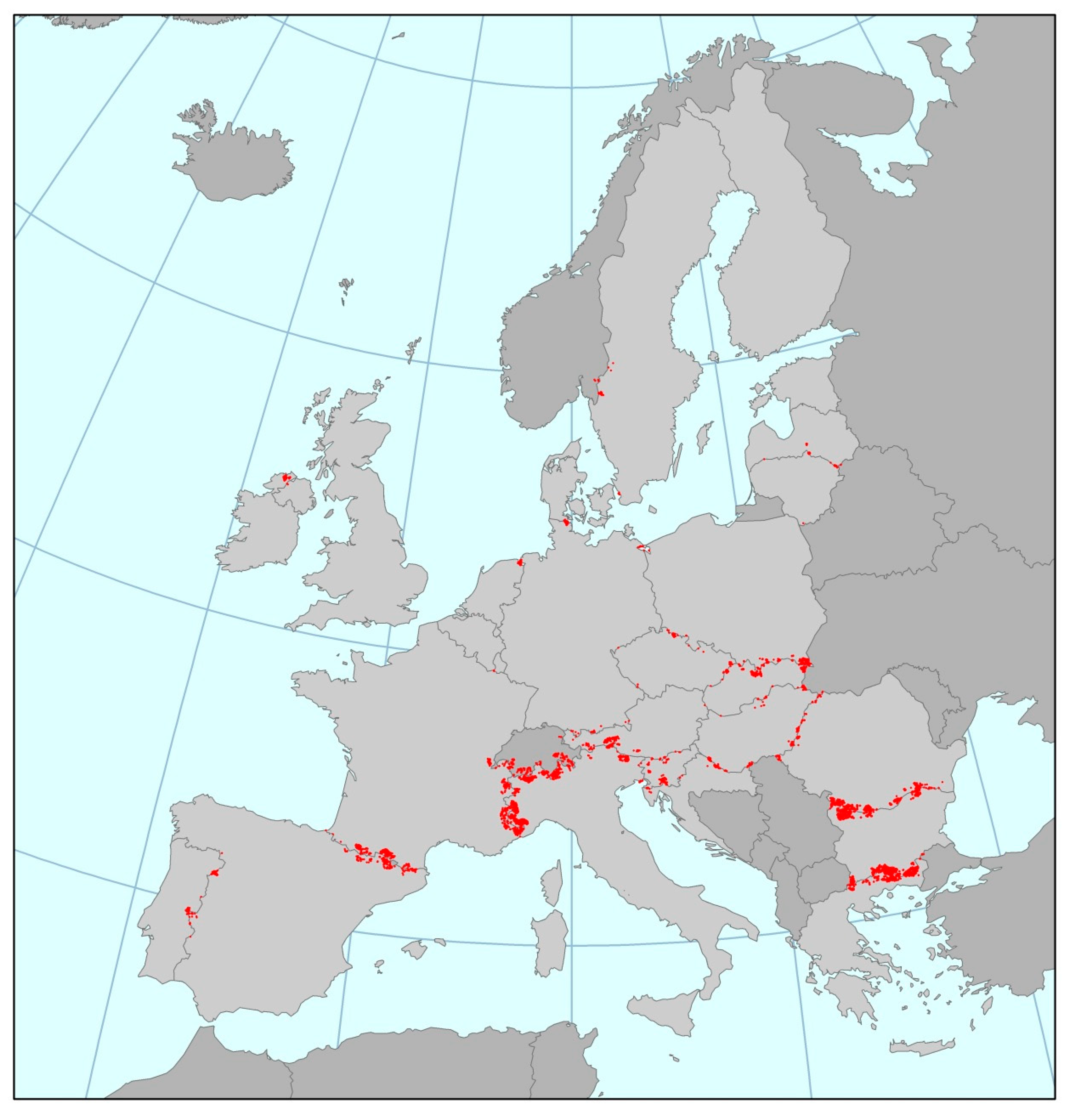
Filtering the results with minimum and maximum values for the national and international side of each cell allows a focus on specific typologies of border areas. For example, Figure 2 maps the zones with high international and low national Potential Accessibility. The thresholds used in this example were a minimum of two million on the international side and a maximum of two million on the national side.

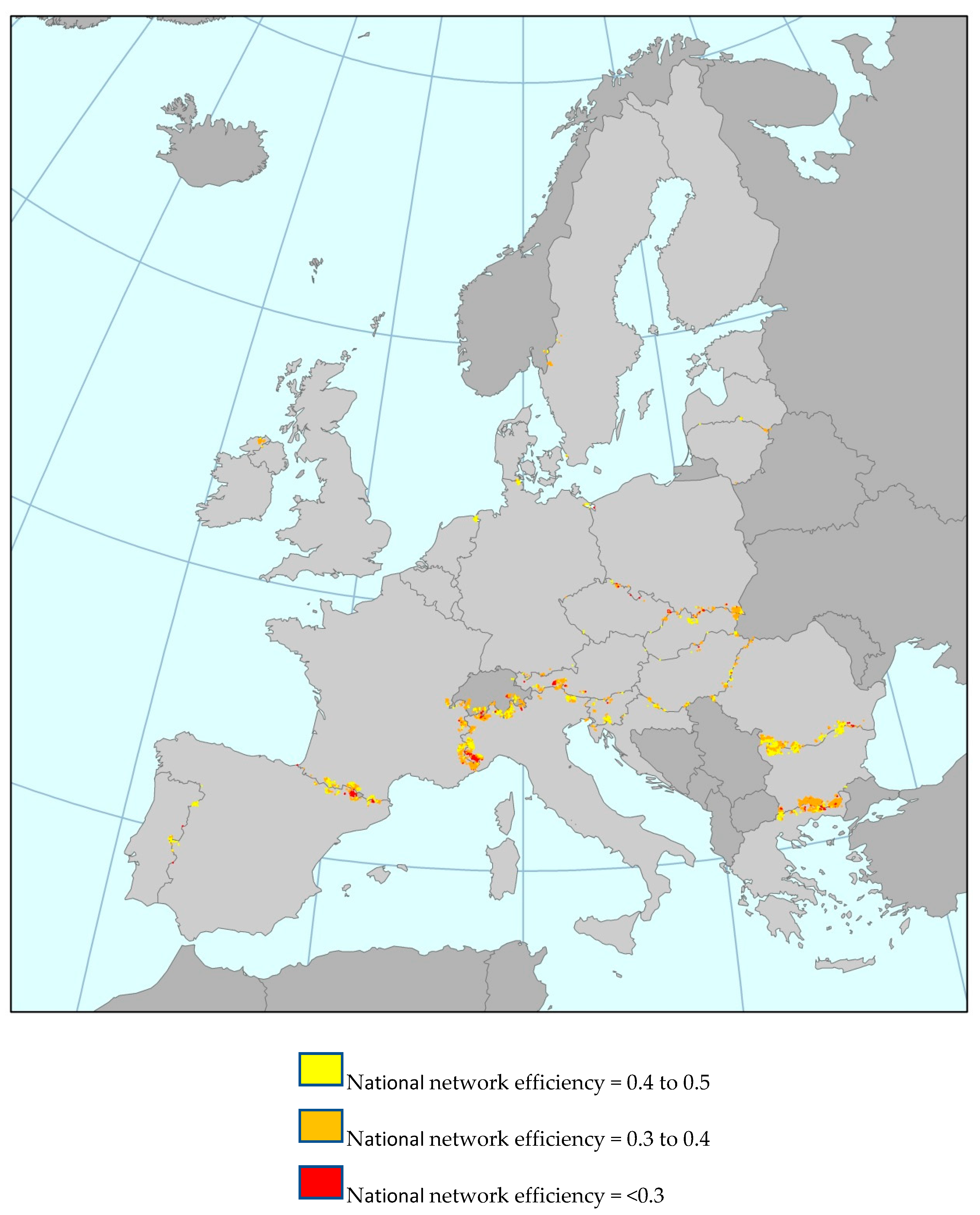
5.3. Network Efficiency

The values of the network efficiency indicator vary significantly depending on local conditions. From the analysis of the distribution of the indicator for the national and international sides of the borders, it is found that the median values of the two sides of the borders are relatively similar, 0.47 and 0.45 respectively, but the variance for the international part is higher. The higher values for international network efficiency correspond to areas very close to border crossings served by highways, while the lowest values to zones that are located close to natural obstacles. In the first case, the morphology and the road design permit a travel time close to the theoretical travel time at maximum speed at straight line. However, in the second case, multiple factors affect the low value of the indicator: Large distance to border crossing, inefficient road design due to difficult morphology, and low operational speed.

Furthermore, the analysis of national and international network efficiency results indicates a rough linear relation between the two. This implies that, in general, the geographic conditions that affect network efficiency have a similar impact on both sides of the border. This could mean that where the two values are similar (ratio ≈ 1) physical obstacles are probably the reasons for a low network efficiency indicator.

The concentration of zones with low values for network efficiency on both sides of the border is evident in Figure 3. Virtually all cells with a low value (<0.3) on the international side have a value lower than 0.5 on the national side as well. The combination of the location of those zones with the elevation map of Europe supports the hypothesis of high concentration on specific borders. Moreover, most of the zones with values lower than 0.3 on both sides of the border (red point on map) are located in mountainous areas.

5.4. Comparison of the Three Accessibility Indicators

Potential accessibility is heavily influenced by distance or travel time, but in this case the relevant impact is expected to be relatively limited as a result of limiting the search of destinations to the settlements within a radius of 75 km from the origins. The results of potential accessibility are, to a large extent, driven by the size of population of destinations. This explains the unexpectedly high results in some regions, but also indicates a weak point of the indicator. The general picture is affected by the fact that by aggregating the results at the level of border regions, the most populated grid cells dominate the totals. Nevertheless, the fact that the indicator is significantly influenced by the population of the destinations and does not focus on the role of the road network make it less suitable to assess transport infrastructure.

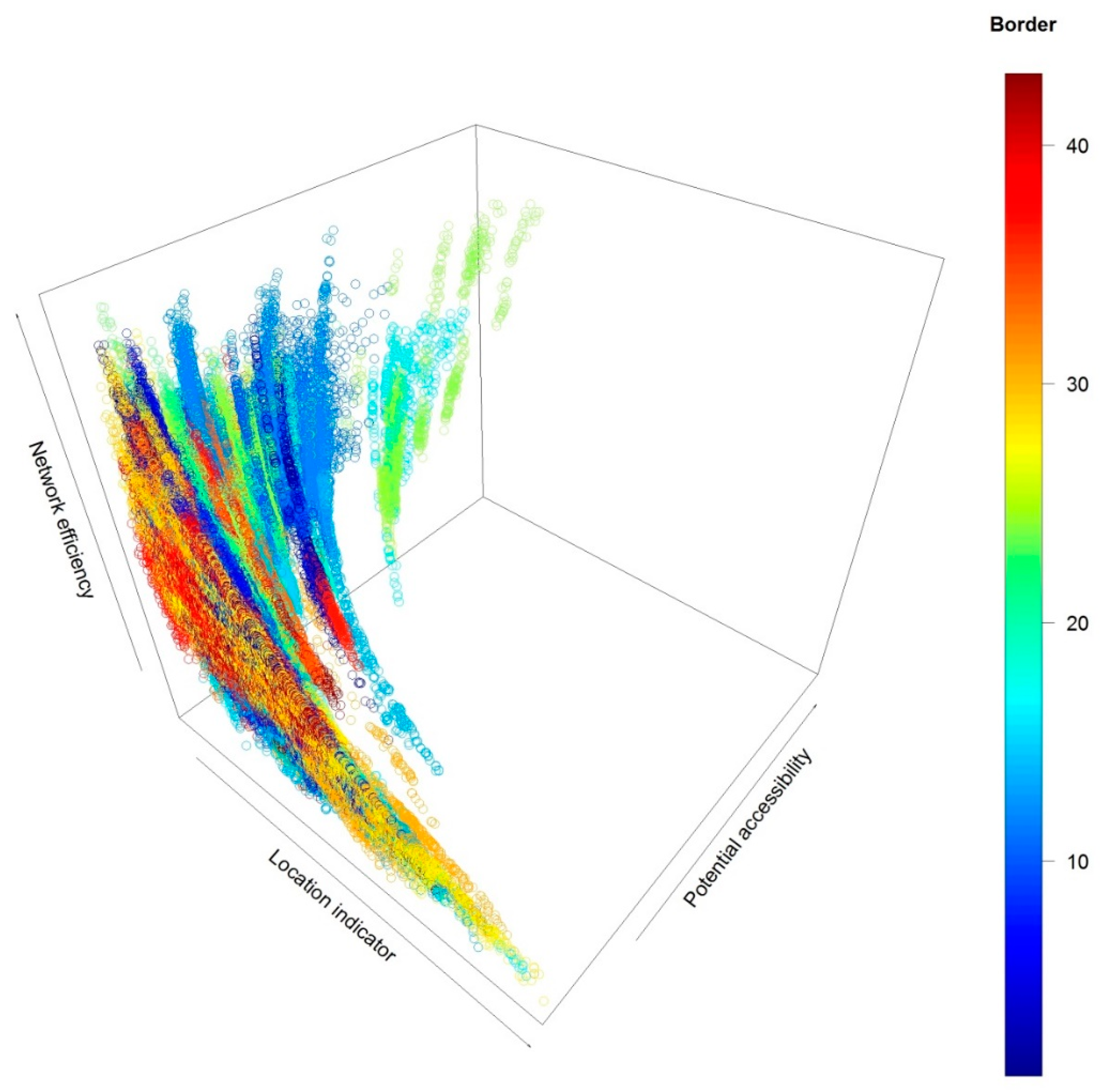
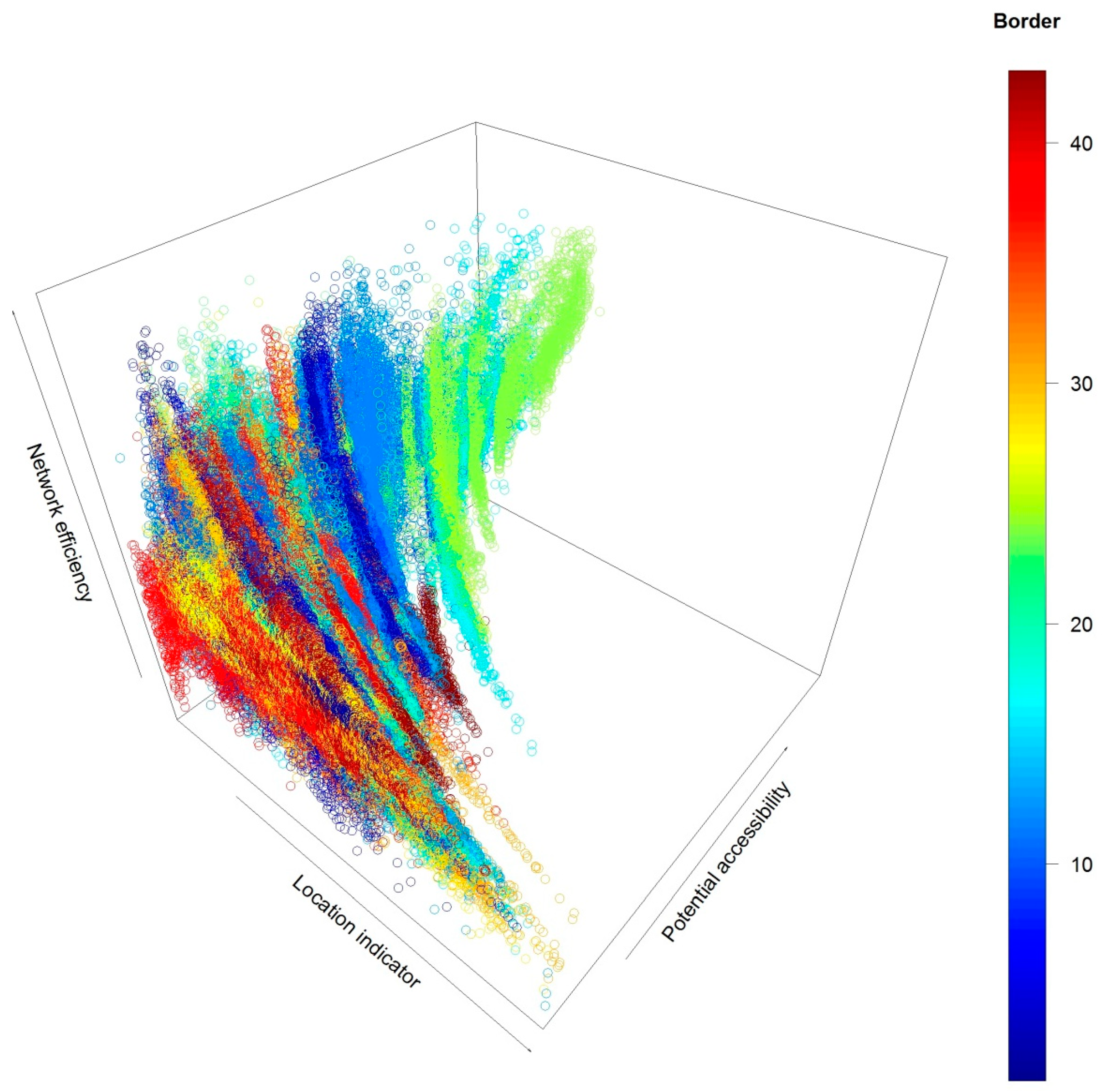
The three indicators present low levels of correlation, both at cross-border (Figure 4) and national (Figure 5) level. The cross-border side of all three indicators has a higher variation than the respective indicator at national level (

Table 1. Summary statistics for accessibility indicators.

	Location Indicator		Potential Accessibility		Network Efficiency
	Cross-Border	National	Cross-Border	National	Cross-Border	National
Mean	0.99	0.81	383 324	906 899	0.45	0.47
Variance	0.073	0.063	2.99 × 1011	1.72 × 1012	0.0068	0.0063

). Nevertheless, while high levels of network efficiency are uniformly spread across various levels of potential accessibility and location indicator levels at national level, the cross-border distribution is much more unbalanced. A relatively small number of cells present high network efficiency, high potential accessibility, and low location indicator (for which low values mean low average travel times) on either side of the border, with the majority corresponding to the national side. These zones correspond to border regions with easy access to highways, are close to large settlements on the other side of the border, and have access to a considerable size of population within 75 km. This is the case mainly for zones on the Netherlands-Germany border. On the other extreme, a relatively large number of zones are considered isolated according to any of the three indicators (i.e., lower values of network efficiency and potential accessibility, higher values of location indicator). The share of zones with such values at national level is considerably lower, confirming the hypothesis that in general, cross-border accessibility is lower than accessibility at national level.

It is worth noting that clusters of zones belonging to the same border can be easily distinguished, probably due to the similarity of the conditions across the whole border that affect (at least) potential accessibility in a similar way. Potential accessibility appears to be the variable that allows the clustering per border to be visible both at national and cross-border level. It also appears that the ordering of the border clusters is roughly the same for both sides of the border, the difference being that the distance between the clusters is much lower at national level. The physical interpretation of this observation is that all three indicators are affected by common factors related to a specific land border, which to a large extent has a similar effect on zones on either side of the border. For example, zones on both sides of the border in a mountainous area are expected to have low values of network efficiency, while border zones located in low density areas would need long travel times (high location indicator) to access major settlements on either side of the border.

6. Application for Policy Analysis

The methodology presented in the preceding sections allows a broad range of analyses related to border regions and/or cross-border collaboration, and can be potentially extended to the exploration of regional development issues in general. While the approach is based on broad accessibility concepts, the indicators used combined with the specific geographic focus selected for this particular implementation allow the generation of relevant quantitative input to policy processes, especially to the ones aiming to:

(1)

Ensure access to a defined level of basic or specific services;

(2)

Increase opportunities and/or economic activity;

(3)

Improve quality of road transport network; and

(4)

Decrease isolation/remoteness.

The approach and the results can be a useful tool for the policy analyst. As the step-by-step description of the approach suggests, a number of the parameters that affect the definition of the interest areas and the operationalization of the indicators are selected empirically by either the policy analysts or the application developers. The translation of policy-side definitions into numerical values involves many approximations and leads to inevitable uncertainty and imprecision. Nevertheless, if those limitations are taken into account, the methodology provides a useful tool that helps quantify and visualize otherwise challenging concepts.

This combination of parameters has been selected empirically, through a close collaboration between the policy analysts and the application developers, including a number of tests using different thresholds. All choices affect the level of relevance and precision of the results, and create a trade-off with computational requirements. Those thresholds appear to provide a detailed enough granulation and a rational approximation of what can be considered a border zone and what is relevant in terms of cross-border interactions.

The indicators proposed here can be useful in describing the existing situation and identifying areas where an improvement in transport infrastructure could potentially lead to improving one or more of the policy objectives set. The three indicators allow flexibility in terms of defining a policy objective and evaluating how this is met. Identifying areas for policy intervention, however, is a heuristic—rather than a deterministic—process, and does not have a clear recipe for reaching the perfect solution. Nevertheless, a combination of suitably formulated policy objectives with a robust set of quantitative indicators can at least guide policy makers towards options that can approximate the aims of the policy objectives.

An example of how this methodology and the resulting dataset can be applied in the context of specific objectives can be the estimation of impacts from network improvement. Upgraded cross-border road links can decrease travel time and improve network efficiency, but would also decrease the Location Indicator and increase the Potential Accessibility indicator. While the decrease in the Location Indicator is lineary correlated with the decrease in travel times, the correlation of the Potential Accessibility indicator with travel time is curvilinear (travel time is in the denominator). Exploring how the two indicators change as a result of improving network efficiency can provide useful input to policy makers.

As a first example, the zones with the highest improvement in terms of Location Indicator as a result of improving network infrastructure are identified. If the same percentage improvement is assumed for all zones in the dataset, the benefit with regard to the reduction of the location indicator in absolute terms will differ, depending on the combinations of the actual values of the location and network efficiency indictators. Assuming a 10% improvement in network efficiency, and using a 10 min threshold value for decreases in the international location indicator, produces a map of the areas where the impact is the highest (Figure 6).

In the second example, the impact in terms of increase in international potential accessibility is explored. A 10% increase in network efficiency is also assumed here, with the threshold of increase in potential accessibility—i.e., the size of the population accessed within 1 hour of travel time—set at 100 thousand (Figure 7).

The two results are visibly different, since two distinct policy objectives are simulated. In the first case, the highest benefit is expected in areas that actually combine low network efficiency and high location indicator (i.e., long travel times). In practical terms, this means that improving roads leads to higher benefits for the most isolated areas. In the second case, the benefit clearly depends on the opportunities already available in the area. The zones already enjoying high accessibility would have a higher benefit than less accessible zones (in absolute terms), for a comparable improvement in road networks.

7. Conclusions

The results of the approach presented here suggest that there is a clear border effect that affects accessibility in border regions. The exploration of different operationalizations of accessibility indicators allows the contribution of physical geographical constraints to be taken into account in order for the underlying connectivity constraints to be revealed. The analysis at a detailed spatial level is complemented by the comparison of indicators within and across national borders, allowing the testing of the hypothesis of the border effect.

One of the main challenges at EU level regarding networks’ integration has been to address relevant inefficiencies by contributing to the development of necessary transport infrastructure. As a result, it is important to identify areas in need, or to classify and benchmark border regions according to accessibility and road infrastructure. In turn, such information can improve the Cost-Benefit Analysis of transport project by adding quantitative indicators that address equity issues, an often underrated aspect of project appraisal.

Physical distance and—by extension—travel time on the road network can be one of the reasons that impede interaction across EU areas close to a land border. There are obviously several reasons why cross-border contacts are more limited than contacts at the same distance within the same country. Centuries of nation building across Europe have led to strong physical, cultural, and linguistic barriers that still persist, even in the context of free movement inside the European Union. In many cases, border regions have been neglected at both national and international level. Priorities for transport infrastructure tended to favor more central zones or as few border crossings as necessary for international trade. As a result, a large part of the internal EU land borders faces the double burden of difficult geographic situation and lack of transport infrastructure investment to reduce isolation. The methodology presented here concentrated on the aspect of connectivity, in particular on exploring ways to measure the quality of cross-border road networks and estimate the potential impact of targeted investments. In most cases, there is a marked difference with regard to the level of cross-border connectivity and accessibility, compared to the respective levels on the national side. Even when taking the influence of local geographic conditions into account, cross-border links are significantly slower and longer than links within the same country.

Aggregating at the level of specific bilateral borders suggests that there is a distinction between older and newer EU member states, central and peripheral European countries, or Western and Eastern European countries. Furthermore, it is observed that a common reason of low accessibility is the existence of natural barriers such as mountains (e.g., in the borders between Greece and Bulgaria, Czech Republic and Poland, Italy and France), rivers (e.g., in the borders between France and Germany, Romania and Bulgaria) or national parks (e.g., in the border between Slovakia and Poland).

The indicators proposed here can provide useful input to policy makers and practitioners in terms of evaluating the current situation, prioritizing areas for intervention, and assessing potential impacts. It should be noted, however, that policy interventions still need to be examined on a case-by-case basis in order to take into account all the relevant characteristics. The approach allows a focus on specific road links, settlements, and physical characteristics, but other factors affecting cross-border collaboration should also be taken into account in additional steps of the analysis. A known limitation of the approach presented here is the use of population as the attraction factor in the operationalization of the accessibility indicators. While this choice—due to data availability reasons—is, to a large extent, suitable for equity analysis, extending the scope with the inclusion of attraction factors that could be proxies of economic activity (e.g., GDP), employment options (e.g., jobs) or access to services (e.g., hospitals) would increase the value and the interpretability of the results. A second limitation of the approach is related to the specific formulations and parameters selected for the analysis. The growing volume of literature in regional studies provides a large number of different approaches for the operationalization of accessibility indicators (see for example, [31,32,33]) or the definition of the parameters used (for example Halás et al., 2014 [11] on the selection of distance-decay functions for daily travel-to-work flows). Future extensions of this work may include a sensitivity analysis of the various parameters used and the exploration of additional indicators that can address accessibility in border regions.

The overall approach can be extended to cover any area by adapting either the extension of the grid used (e.g., accessibility of wider zones or even the whole of the EU), or the size of the zone of interest (to calculate indicators using different formulations or attraction factors). The results can be easily combined with other policy support tools for tailored multi-criteria analysis. There are two aspects in regional policy that the methodology presented here addresses. On the one hand, the accessibility indicators provided can help in identifying where intervention may be required in order to improve equity and increase access to opportunities. On the other hand, they can assist in the prioritization of interventions or investments within a specific area. For example, under conditions of restricted budget, accessibility indicators can provide valuable information as regards the most effective or most efficient investment.