Determining Key Agricultural Strategic Factors Using AHP-MICMAC

Abstract

Agriculture is an irrefutable part of food policy. This paper aims to introduce an integrated method using MICMAC and AHP techniques to deal with understanding the key strategic variables of agricultural system. MICMAC was used to determine the classifications of variables and AHP was applied to weigh these classifications. MICMAC is a structural analysis tool used to structure ideas and AHP is an effective tool to deal with complex decision making and helps decision-makers making the best decision. The results show that strategic variables had different types of influence and direct, indirect, and potential dependencies did not have the same importance. AHP-MICMAC not only considers these differences, but also puts a total priority weight for each variable. These characteristics have an important role in forming strategies and scenarios for agricultural development. Therefore, the case of Iran was used to illustrate the application of MICMAC aiming to supply instructions for the development of agriculture system.

1. Introduction

Agriculture is a complex system [1], but due to the risky and diverse nature of agriculture in developing countries, the systemic complexity is greater [2]. In a complex system, there are a variety of autonomous actors, just as a variety of actors and processes of adaptation can be found within the agricultural system [3]: humans (farmers, laborers, consumers, policy makers, experts, agents, etc.) [4,5], economy (market, cost, income, etc.) [6], nature (weather and climate, topology, etc.) [7,8,9], policy (plans, policies, strategies, etc.) [10], regulations (heritage, property rights, trade, etc.) [11], infrastructures (transportation, processing, saving, marketing, insurance, etc.) [12,13,14], inputs (land, water, seed, fertilizer, technology, etc.) [5,15,16,17].

Determining what kind of factors or variables need to be considered by decision and policy-makers is challenging [18]. Policy-makers tend to use different criteria and methodologies in order to determine strategic variables and factors influencing agricultural development [19]. Yet, because of the complexity of agricultural systems, the ability of researchers and policy-makers to prioritize variables is often limited. As a result, the majority of previous studies have dealt with this subject from a limited point of view (such as insurance or risk management) and on a micro level (such as a single farmer or farm). For instance, Pascucci and de-Magistris [20] implemented a multivariate probit model to evaluate the effects of different types of agricultural extension and innovation systems on farmers’ strategies in Italy. Allen [21] used the bet-hedging model and Neo-Darwinian theory (risk management strategies) to offer a way of evaluating the historical development of dryland agriculture as well as the long-term outcomes of variant agronomic strategies in Kona, Hawaii. Qingshui and Xuewei [22] and Zhou et al. [23] used empirical research to develop and improve strategies for the agricultural insurance system in rural of China by considering income sources, mean of production, labor opportunities, government supports, and communication channels. In Anambra, Nigeria, Amadi [14] evaluated the impact of rural road construction and its adjacent infrastructures (electricity, pipe-borne water and irrigation technology) that were used as a strategy for rural and agricultural development. Ames [4] emphasized investment in human capital as a strategy for implementing changes in agricultural policy, research, and extension activities.

Most of these studies only considered a few limiting factors or variables and their intensities, but none of them attended to characteristics such as dependent or independent variables, direct or indirect impacts, or the weight of each variable or factor. These characteristics have an important role in forming strategies and scenarios for agricultural development. As a result, there is a methodological gap that the present study aims to fill by providing a new integrated method. This new integrated method applies Impact Matrix Cross-reference Multiplication to a classification (MICMAC) [24,25] and analytic hierarchy process (AHP) [26]. The case of the agricultural system in Iran is used to show the application of this new methodology. Agriculture is one of the most important sectors of the Iranian economy, accounting for about 11% of GDP, 23% of the employed population, and 15% of the foreign exchange revenue (form non-oil exports). In addition to the fact that products from the agriculture and animal husbandry have been major export commodities, including pistachios, raisins, and even carpets. About 20% of Iran is arable, with some northern and western areas that support rain-fed agriculture, while other areas require irrigation.

Each of these methods alone has advantages and limitations for example MICMAC can investigate multiple variables at the same time, but it does not give an overall priority score for each variable. On other side, AHP considers only direct impact of variables, but it gives and overall priority score for each variable. This study has tried to overcome these constraints and to consider their advantages by combining them and proposing an integrated method. It is our hope that this new integrated method will supply instructions for the development of agriculture, and find wider applications in complex systems.

2. Materials and Methods

2.1. MICMAC Method

The Impact Matrix Cross-Reference Multiplication Applied to a Classification (MICMAC) is a structural analysis tool used to structure ideas and as a forecasting method created by Michel Godet. MICMAC can be considered a qualitative system dynamics approach [27] and provides the possibility to describe a system with the help of a matrix connecting all its components. By studying these relations, the method also makes it possible to reveal the variables essential to the evolution of the system. It is possible to use MICMAC as an aid for reflection and/or for decision making, or as a part of a more complex forecasting activity [28]. MICMAC tries to pinpoint the independent and dependent variables by building a typology in both direct and indirect classifications [28]. In MICMAC we depart from the definition of the system’s variables and their interrelations, both of which were provided by experts. This method has at least three main phases [25,28,29]:

Phase (1) Considering all the variables: This phase begins by considering all of the variables or factors that characterize the studied system. Brainstorming and intuitive methods or a panel of experts are useful methods for this phase. A detailed explanation of the variables is also essential because it will allow the relations between these variables to be perceived better in the analysis. The final output of this phase is a homogeneous list of internal and external variables (Table 1) and should not exceed more than 70 to 80 variables.

Table 1. A sample list of internal and external variables.

Type of Variables	Group Name (if it is necessary)	No	Symbol	Description (Lable)
Internal variables	Economic	1	Var1	Income …
		2	Var2	…
	Social	3	Var3	Participation …
		4	Var4	…
External variables	…	5	Var5	…
		6	Var6	…
	…	7	Var7	…
		8	Var8	…

Phase (2) Constructing the structural analysis matrix (description of the relations between the variables): In a systemic vision, a variable is a part of the relational web. A structural analysis matrix is a squared matrix that allows the variables to connect directly. The cells store the degree of influence between each pair of variables, i and j (0 no influence, 1 weak influence, 2 medium, 3 strong and P potential) (Table 2) (A group of experts filled this matrix). This filling-in phase helps place N × (N − 1) questions for N variables. Additionally, the questioning procedure not only enables us to avoid errors, but also helps us organize and classify ideas by creating a common group language. It also allows for the variables to be redefined and therefore makes analysis of the system more accurate. Figure 1 indicates the structural diagram of Table 2.

Table 2. A sample structural analysis matrix (M) with four variables.

Variables	Var1	Var2	Var3	Var4	Influence
Var1	0	0	1	3	4
Var2	1	P	1	0	2
Var3	0	2	0	0	2
Var4	0	1	3	0	4
Dependence	1	3	5	3	-

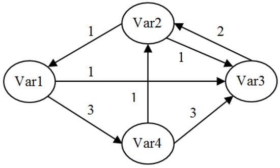
Figure 1. A structural diagram (based on the data of Table 2).

Phase (3) Identification of the key variables: This phase consists of identifying variables essential to the system’s development. At first, this was accomplished by using direct classification, then through indirect classification and, finally, by potential classification. Comparing the hierarchy of variables in the various types of classifications (direct, indirect, and potential) is a rich source of information. It enables us not only to confirm the importance of certain variables, but also to uncover variables which play an important role yet were not identifiable through direct classification in the initial process. The direct influence and dependence of a variable are the aggregate of its row and column. The sum of each row indicates the importance of the influence of a variable on the whole system (other variables) (Equation (1)) and the sum of a column indicates the degree of dependence of a variable on the other variables (Equation (2)):

$$D{I}_j={\displaystyle \sum }_{j=1}^n{V}_{ij} i \mathrm{and} j = 1,2,\dots ,n$$

(1)

$$D{D}_i={\displaystyle \sum }_{i=1}^n{V}_{ij}i \mathrm{and} j = 1,2,\dots ,n$$

(2)

Indirect classification is obtained after increasing the power of the matrix M (matrix multiplication M² = M × M, M³ = M × M × M, and so on). For example, in Figure 1 Var1 has a direct (DI₁₃ = V₁→V₃ = 1) and indirect (II₁₃ = V₁→V₄→V₃) influence on Var3. To calculate indirect influence or dependence of a path, we should increase the power of the matrix by considering the number of paths and loops of length (1, 2, …, N) that result from or arrive at each variable (for example, for II₁₃ = V₁→V₄→V₃, the power of the matrix should be Equation (2)). The MICMAC then allows us to study the diffusion of the impacts through the paths and loops of feedback. Generally, the classification becomes stable after a degree of multiplication of 3, 4 or 5 [29].

M =	0	0	1	3	→ M2 =	0	5	9	0
	1	0	1	0		0	2	1	3
	0	2	0	0		2	0	2	0
	0	1	3	0		1	6	1	0

A potential direct or indirect classification is a direct or indirect relation (influence or dependence) that considers potential relations. To calculate potential relations, we ought to first replace P in matrix M with an ordinal number (1, 2, or 3, depending on the intensity of influence) and then increase the power of the new matrix to a point where the row and column priorities become stable. If there is no potential influence or dependence, the degree of potential relations will be equal to existing relations. In simple terms, feedback loops may take a number of iterations to come to a settled state. The number of times that the matrix can be multiplied depends upon how long it takes to stabilize.

MICMAC compared to the results (direct, indirect, and potential classification) provides the possibility to confirm the importance of variables. The main result of this phase is a matrix m × n (Table 3), which we named matrix R; where m is the number of various types of relations (various types of classifications). Here it includes eight types: Direct Influence (DI), Indirect Influence (II), Direct Dependence (DD), Indirect Dependence (ID), Potential Direct Influences (PDI), Potential Indirect Influence (PII), Potential Direct Dependence (PDD), and Potential Indirect Dependence (PID). N represents the number of variables. A comparison of the hierarchy within the variables provides a rich source of information.

Table 3. Identification of the key variables according to various types of classifications (Matrix R).

Matrix R	DI	II	DD	ID	PDI	PII	PDD	PID
V1
V2
:
Vn

2.2. AHP Method

The analytic hierarchy process (AHP) is a structured technique developed by Thomas L. Saaty in the 1970s. It is an effective tool when dealing with complex decision making and helps decision-makers to set priorities and make the best decision. AHP uses a series of paired comparisons to reduce complex decisions. Then, by synthesizing the results, it helps capture both the subjective and objective aspects of a decision. Additionally, AHP is used to reduce bias in a decision making process and incorporates a useful technique that checks the consistency of the decision-maker’s judgments [26,30,31].

The AHP can be implemented through the following steps:

• Define the problem and determine the objectives, criteria, sub-criteria, and alternatives.
• Structure the decision hierarchy from the top (the goal of the decision), down (the alternatives).
• Construct a set of paired comparison matrices. Each element on an upper level is used to compare the elements at the level immediately below it.
• Compute the vector of criteria weights.
• Compute the matrix of option scores. For each element in the level below, add its weighed values and obtain its overall or global priority.
• Rank the options (alternatives).

Each step will be described in detail. We assume that the m evaluation criteria are considered as evaluated n options or alternatives (in our study, 45 variables).

(1) Define the problem: Our problem or goal was determining the strategic variables of agricultural development based on various types of classifications.

(2) Structure the decision hierarchy: The structure of our decision hierarchy is shown in Figure 2. This hierarchical process includes three levels: (a) Goal (in our study it was to determine the strategic variables of an agricultural system), (b) criteria (in our study they were eight types of classifications: DI, II, DD, ID, PDI, PII, PDD, and PID), and (c) alternative variables.

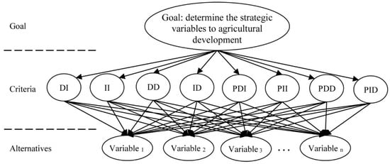
Figure 2. The structure of the decision hierarchy.

(3) Create a paired comparison matrix (A): Matrix A is a m × m matrix. Each entry, a_ij, presents the importance of the ith criterion relative to the jth criterion. If a_ij = k and k > 1, it means that the ith criterion is k times more important than the jth criterion, while if a_ij = k and k < 1, it means that the ith criterion is k times less important than the jth criterion. If k = 1, then the two criteria have the same importance. The entries a_ij and a_ji satisfy this constraint, a_ij × a_ji = 1 (a_ij = 1/a_ji). The relative importance between two criteria is measured according to a numerical scale, from 1 to 9 (1 for equal importance of i and j, …, 9 absolutely i is more important than j). The consistency index (CI) [31] was used to check the reliability of the paired comparisons.

		a1	a2	..	aj
A =	a1	a11	a12	..	a1j
	a2	a21	a22	..	a2j
	ai	ai1	ai2	..	aij

(4) Compute the vector of criteria weight: Once matrix A is built, it should be normalized. To this purpose, the sum of the entries on each column should be made equal to 1. In the resulting matrix (A_norm), each entry ā_ij is computed as (Equation (3)):

$${\overline{a}}_{ij}=\frac{a_{ij}}{{{\displaystyle \sum }}_{j=1}^m{a}_{ij}}$$

(3)

Finally, the criteria weight vector w is built by averaging the entries in each row of matrix A_norm (Equation (4)).

$$w_i=\frac{{{\displaystyle \sum }}_{i=1}^m{\overline{a}}_{ij}}{m}$$

(4)

(5) Compute the matrix of option scores: This matrix is a m × n real matrix (S). Each entry s_ij of S represents the score of the ith option with respect to the jth criterion. In our study this matrix was the output of the MICMAC method and was a 8 × 45 matrix (8 types or relations and 45 strategic variables).

(6) Rank the options or alternatives (variables): in this phase a vector v of global scores is obtained by multiplying matrix S and vector w, i.e., v_j = S × w_i.

2.3. AHP-MICMAC Integrated Method

Although the MICMAC method is useful when identifying key variables and it gives us the priority of each variable according to different types of relations (from direct influence to potential indirect dependence), it couldn’t calculate a proper weight for the types of relations or an overall priority ranking with respect to these weights of each variable. Thus, we introduced an integrated method (AHP-MICMAC) to deal with this problem. As Figure 3 indicates, AHP-MICMAC can be implemented in eight simple consecutive steps:

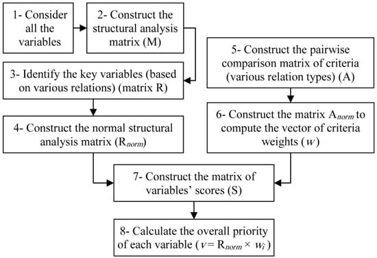
Figure 3. The process of the AHP-MICMAC method.

(1) Consider all the variables: At first, we prepared a list of important variables extracted from literature review. Then, we organized a panel of 10 experts (including five faculty members of Agricultural Economics and Development at University of Tehran and five experienced experts of Agricultural Ministry) in order to prepare a final list of all variables that are fundamental for the development of agriculture in Iran. Brainstorming among the group, the panel finally extracted 45 variables as the key variables of agricultural development (Table 4).

Table 4. The key variables for agricultural development.

Label	Variable	Label	Variable
V01	The demand for agricultural products	V24	Farmers’ knowledge, awareness and skills
V02	Consumers’ interest and motivation	V25	Agricultural extension and education
V03	Consumers’ knowledge and awareness	V26	Agricultural research
V04	Consumers’ purchasing power	V27	The amount of water resources
V05	Consumers’ access to agricultural products	V28	Water efficiency
V06	Marketing	V29	Climate (temperature and precipitation)
V07	A proper network of markets	V30	Technology
V08	A price system and pricing	V31	Agricultural support system
V09	Transportation and communications	V32	Agricultural land area
V10	Data and Information network	V33	Agricultural land laws and regulations
V11	Processing and packaging	V34	Soil texture
V12	Agricultural products price	V35	Topology
V13	A system for consumer protection	V36	Land fragmentation
V14	Commercial infrastructure	V37	Optimum use of inputs (seeds, fertilizers, etc.)
V15	Storage facilities	V38	The price of production inputs
V16	Trade incentives and restrictions	V39	Existence of rural job opportunities
V17	The amount of agricultural production	V40	The number of agricultural labor
V18	Production costs	V41	The international prices of agricultural products
V19	Government policies and programs	V42	Involving farmers in agricultural development
V20	Quality agricultural products	V43	Farmers organizing and institutionalizing
V21	Farmers’ interest and motivation	V44	Disasters (droughts, floods, earthquakes, etc.)
V22	Financial ability of farmers	V45	Crop insurance
V23	Rural welfare and comforting

(2) Construct the structural analysis matrix (M): We constructed a 45 × 45 matrix of key variables and asked a panel of experts to score the degree of influence between each pair of variables on a scale from 0 to 3 (0 no influence; 1, weak influence; 2, medium influence; and 3, strong influence) (Table 5).

Table 5. A part of the constructed structural analysis matrix (M).

M	V01	V02	V03	V04	V05	V06	V07	V08	V09	V10	V11	V12	V13	V14	V15
V01	0	0	0	0	0	3	3	2	2	0	2	3	2	2	2
V02	3	0	2	0	0	1	0	0	0	0	2	2	0	1	0
V03	2	2	0	0	0	0	0	0	0	0	2	0	0	0	0
V04	3	2	1	0	2	0	0	2	0	0	0	2	3	0	0
V05	2	1	0	0	0	0	0	0	0	0	0	0	1	0	0
V06	3	2	1	0	2	0	3	2	2	2	3	3	0	2	3
V07	3	0	0	0	3	3	0	0	2	1	0	0	2	0	2
V08	3	2	0	0	0	2	0	0	0	0	0	1	3	0	0
V09	1	0	0	0	3	2	2	0	0	0	2	2	0	2	1
V10	2	2	2	0	1	2	0	0	0	0	0	1	0	0	0
V11	3	2	0	0	1	3	0	0	0	0	0	2	0	0	2
V12	3	2	0	2	0	2	2	3	0	0	2	0	2	0	2
V13	3	3	2	2	2	1	0	1	0	0	0	2	0	1	2
V14	0	0	0	0	2	2	2	1	2	1	3	2	0	0	3
V15	0	0	0	0	2	2	0	2	0	0	2	2	0	0	0

(3) Identify the key variables (based of various relations) (matrix R): Using MICMAC software (Version 6.1.2 [32]), we identified the key variables based on 8 different types of relations: Direct Influence (DI), Indirect Influence (II), Direct Dependence (DD), Indirect Dependence (ID), Potential Direct Influences (PDI), Potential Indirect Influence (PII), Potential Direct Dependence (PDD), and Potential Indirect Dependence (PID) (Table 3 and Table 6).

Table 6. The key variables based on various relations (matrix R and matrix R_norm).

Matrix	Non-Normal (Matrix R)								Normal (Matrix Rnorm)
	DI	II	DD	ID	PDI	PII	PDD	PID	DI	II	DD	ID	PDI	PII	PDD	PID
V01	243	237	314	323	243	239	314	321	0.024	0.024	0.031	0.032	0.024	0.024	0.031	0.032
V02	114	122	171	176	114	123	171	174	0.011	0.012	0.017	0.018	0.011	0.012	0.017	0.017
V03	71	67	64	51	71	67	64	50	0.007	0.007	0.006	0.005	0.007	0.007	0.006	0.005
V04	157	146	64	80	157	147	64	78	0.016	0.015	0.006	0.008	0.016	0.015	0.006	0.008
V05	64	65	171	176	64	65	171	174	0.006	0.007	0.017	0.018	0.006	0.007	0.017	0.017
V06	386	361	336	382	386	363	336	381	0.039	0.036	0.034	0.038	0.039	0.036	0.034	0.038
V07	200	193	143	166	200	194	143	166	0.020	0.019	0.014	0.017	0.020	0.019	0.014	0.017
V08	164	184	236	270	164	184	236	269	0.016	0.018	0.024	0.027	0.016	0.018	0.024	0.027
V09	200	183	193	186	200	183	193	185	0.020	0.018	0.019	0.019	0.020	0.018	0.019	0.019
V10	264	265	121	123	264	264	121	123	0.026	0.027	0.012	0.012	0.026	0.026	0.012	0.012
V11	250	228	343	379	250	230	343	377	0.025	0.023	0.034	0.038	0.025	0.023	0.034	0.038
V12	343	325	450	478	343	325	450	478	0.034	0.033	0.045	0.048	0.034	0.033	0.045	0.048
V13	257	236	135	150	257	237	135	149	0.026	0.024	0.014	0.015	0.026	0.024	0.014	0.015
V14	271	254	114	121	271	255	114	120	0.027	0.025	0.011	0.012	0.027	0.026	0.011	0.012
V15	178	181	278	320	178	181	278	318	0.018	0.018	0.028	0.032	0.018	0.018	0.028	0.032
V16	250	237	185	196	250	238	185	195	0.025	0.024	0.019	0.020	0.025	0.024	0.019	0.020
V17	336	320	672	578	336	321	672	582	0.034	0.032	0.067	0.058	0.034	0.032	0.067	0.058
V18	271	275	436	389	271	275	436	393	0.027	0.028	0.044	0.039	0.027	0.028	0.044	0.039
V19	565	505	472	404	565	507	472	408	0.057	0.051	0.047	0.040	0.057	0.051	0.047	0.041
V20	243	223	393	336	243	224	393	339	0.024	0.022	0.039	0.034	0.024	0.022	0.039	0.034
V21	128	151	436	385	128	150	436	388	0.013	0.015	0.044	0.039	0.013	0.015	0.044	0.039
V22	271	263	429	422	271	263	429	422	0.027	0.026	0.043	0.042	0.027	0.026	0.043	0.042
V23	193	188	207	201	193	186	207	202	0.019	0.019	0.021	0.020	0.019	0.019	0.021	0.020
V24	336	335	121	135	336	334	121	134	0.034	0.034	0.012	0.014	0.034	0.033	0.012	0.013
V25	286	279	264	285	286	279	264	283	0.029	0.028	0.026	0.029	0.029	0.028	0.026	0.028
V26	214	254	193	240	214	253	193	238	0.021	0.025	0.019	0.024	0.021	0.025	0.019	0.024
V27	243	259	157	150	243	258	157	150	0.024	0.026	0.016	0.015	0.024	0.026	0.016	0.015
V28	214	231	228	224	214	230	228	225	0.021	0.023	0.023	0.022	0.021	0.023	0.023	0.023
V29	243	251	42	43	243	250	42	43	0.024	0.025	0.004	0.004	0.024	0.025	0.004	0.004
V30	393	372	264	265	393	373	264	264	0.039	0.037	0.026	0.027	0.039	0.037	0.026	0.026
V31	250	274	185	195	250	273	185	195	0.025	0.027	0.019	0.020	0.025	0.027	0.019	0.020
V32	200	209	243	215	200	208	243	218	0.020	0.021	0.024	0.022	0.020	0.021	0.024	0.022
V33	157	181	114	109	157	180	114	109	0.016	0.018	0.011	0.011	0.016	0.018	0.011	0.011
V34	128	135	135	115	128	134	135	116	0.013	0.014	0.014	0.012	0.013	0.013	0.014	0.012
V35	114	121	0	0	114	122	0	0	0.011	0.012	0.000	0.000	0.011	0.012	0.000	0.000
V36	135	146	85	86	135	145	85	86	0.014	0.015	0.009	0.009	0.014	0.015	0.009	0.009
V37	150	152	243	199	150	152	243	202	0.015	0.015	0.024	0.020	0.015	0.015	0.024	0.020
V38	114	134	150	166	114	133	150	165	0.011	0.013	0.015	0.017	0.011	0.013	0.015	0.017
V39	85	73	128	178	85	72	128	177	0.009	0.007	0.013	0.018	0.009	0.007	0.013	0.018
V40	92	109	200	249	92	108	200	248	0.009	0.011	0.020	0.025	0.009	0.011	0.020	0.025
V41	85	97	185	194	85	97	185	193	0.009	0.010	0.019	0.019	0.009	0.010	0.019	0.019
V42	228	247	135	143	228	246	135	142	0.023	0.025	0.014	0.014	0.023	0.025	0.014	0.014
V43	371	390	207	199	371	390	207	198	0.037	0.039	0.021	0.020	0.037	0.039	0.021	0.020
V44	357	348	35	3	357	348	35	4	0.036	0.035	0.004	0.000	0.036	0.035	0.004	0.000
V45	164	174	300	294	164	173	300	293	0.016	0.017	0.030	0.029	0.016	0.017	0.030	0.029
Sum	9978	9980	9977	9979	9978	9979	9977	9975	1	1	1	1	1	1	1	1

(4) Construct the normal structural analysis matrix (R_norm): During this phase, Equation (3) was applied to matrix R to convert to matrix R_norm (Table 6).

(5) Construct the paired comparison matrix of criteria (A): Since the MICMAC method includes eight different types of classifications (DI, II, DD, ID, PDI, PII, PDD and PID), there are eight criteria. Therefore, the paired comparison matrix A is an 8 × 8 matrix. The following matrix is the constructed matrix A for this study:

		DI	II	DD	ID	PDI	PII	PDD	PID
A=	DI	1.00	2.00	2.00	4.00	2.00	4.00	4.00	8.00
	II	0.50	1.00	1.00	2.00	1.00	2.00	2.00	4.00
	DD	0.50	1.00	1.00	2.00	1.00	2.00	2.00	4.00
	ID	0.25	0.50	0.50	1.00	0.50	1.00	1.00	2.00
	PDI	0.50	1.00	1.00	2.00	1.00	2.00	2.00	4.00
	PII	0.25	0.50	0.50	1.00	0.50	1.00	1.00	2.00
	PDD	0.25	0.50	0.50	1.00	0.50	1.00	1.00	2.00
	PID	0.13	0.25	0.25	0.50	0.25	0.50	0.50	1.00

(6) Construct the matrix A_norm to compute the vector of criteria weights (w): The matrix A_norm and the vector of criteria weights (w) were calculated, respectively, using Equations (3) and (4). The matrix and vector for our study are indicated below:

		DI	II	DD	ID	PDI	PII	PDD	PID	wi
Anorm =	DI	0.296	0.296	0.296	0.296	0.296	0.296	0.296	0.296	0.296
	II	0.148	0.148	0.148	0.148	0.148	0.148	0.148	0.148	0.148
	DD	0.148	0.148	0.148	0.148	0.148	0.148	0.148	0.148	0.148
	ID	0.074	0.074	0.074	0.074	0.074	0.074	0.074	0.074	0.074
	PDI	0.148	0.148	0.148	0.148	0.148	0.148	0.148	0.148	0.148
	PII	0.074	0.074	0.074	0.074	0.074	0.074	0.074	0.074	0.074
	PDD	0.074	0.074	0.074	0.074	0.074	0.074	0.074	0.074	0.074
	PID	0.037	0.037	0.037	0.037	0.037	0.037	0.037	0.037	0.037
		1.000	1.000	1.000	1.000	1.000	1.000	1.000	1.000	1.000
	Inconsistency Index = 0.000

(7) Compute the matrix of the variables’ scores (construct the matrix S): Matrix S is a matrix that includes the matrix R_norm and the vector of criteria weights (w). Table 7 represents a part of this matrix. The first row is include the criteria weights and the rest rows are include the normalized scores of the variables. Constructing this table will help researchers to calculate the overall priority of each variable.

Table 7. A part of matrix S.

wi	0.296	0.148	0.148	0.074	0.148	0.074	0.074	0.037
Rnorm	DI	II	DD	ID	PDI	PII	PDD	PID
V01	0.024	0.024	0.031	0.032	0.024	0.024	0.031	0.032
V02	0.011	0.012	0.017	0.018	0.011	0.012	0.017	0.017
V03	0.007	0.007	0.006	0.005	0.007	0.007	0.006	0.005
V04	0.016	0.015	0.006	0.008	0.016	0.015	0.006	0.008
V05	0.006	0.007	0.017	0.018	0.006	0.007	0.017	0.017
:	:	:	:	:	:	:	:	:
V45	0.016	0.017	0.030	0.029	0.016	0.017	0.030	0.029

(8) Calculate the overall priority of each variable: In order to calculate the overall priority for each variable, we mulitplied matrix R_norm on vector w_i (v = R_norm × w_i). Table 8 includes the total priority (TP = OPI + OPD), overall priority of influences (OPI = DI + II + PDI + PII), and the overall priority of dependences (OPD = DD + ID + PDD + PID) for all variables. To determine the model’s validity (the differences between model results and the realities), we asked the experts to judge the results of the proposed integrated method (AHP-MICMAC).

Table 8. The total (TP), overall influences (OPI) and overall dependences (OPD) priorities.

Var	OPI	OPD	TP *	Var	OPI	OPD	TP	Var	OPI	OPD	TP
V19	0.036	0.015	0.051	V21	0.009	0.014	0.023	V07	0.013	0.005	0.018
V17	0.022	0.021	0.044	V16	0.016	0.006	0.023	V29	0.016	0.001	0.018
V12	0.023	0.015	0.038	V28	0.015	0.008	0.022	V37	0.010	0.008	0.018
V06	0.025	0.012	0.037	V26	0.015	0.007	0.022	V33	0.011	0.004	0.015
V30	0.026	0.009	0.035	V27	0.017	0.005	0.022	V40	0.007	0.007	0.014
V18	0.018	0.014	0.032	V10	0.018	0.004	0.022	V02	0.008	0.006	0.014
V22	0.018	0.014	0.032	V15	0.012	0.010	0.022	V38	0.008	0.005	0.013
V43	0.025	0.007	0.032	V14	0.018	0.004	0.022	V34	0.009	0.004	0.013
V20	0.016	0.013	0.028	V13	0.017	0.005	0.021	V04	0.010	0.002	0.013
V11	0.016	0.012	0.028	V32	0.014	0.008	0.021	V41	0.006	0.006	0.012
V25	0.019	0.009	0.028	V45	0.011	0.010	0.021	V36	0.009	0.003	0.012
V01	0.016	0.011	0.027	V42	0.016	0.005	0.020	V39	0.005	0.005	0.010
V24	0.022	0.004	0.027	V08	0.011	0.008	0.020	V05	0.004	0.006	0.010
V44	0.024	0.001	0.024	V23	0.013	0.007	0.020	V35	0.008	0.000	0.008
V31	0.017	0.006	0.024	V09	0.013	0.006	0.019	V03	0.005	0.002	0.007
Sum									0.667	0.333	1.000

* sorted by TP column.

3. Results and Discussion

3.1. The Weights of Various Types of Classifications

In the AHP-MICMAC method, unlike the MICMAC method, various classes of variables do not have the same weights. As matrix A_norm shows, the direct influences (DI) and potential indirect dependence (PID), respectively, have had the highest (0.296) and the lowest (0.037) weights among the various types of classifications. Additionally, the weights of II, DD, and PDI classes (0.148) were the same as each other, but their weights were two times more than the ID, PII, and PDD classes (0.074), which have the same weight. Based on Table 8, the sum of the overall priorities of influences (0.667) is two times more than the sum of the overall priorities of dependences (0.333). This means that the experts believe the characteristics of the influences of variables are more important than the characteristics of the dependencies of variables of agricultural development. It is also true for the sum of potential weights (PDI + PII + PDD + PID = 0.667) compared to actual weights (DI + II + DD + ID = 0.333). As is shown in the following section, the application of these weights may change the priority of variables.

3.2. The Most Influence and Dependence Variables

Table 6 demonstrates that for an agricultural development system, the most and the least direct and indirect influence variables (both actual and potential) were, respectively, V19 (government policies and programs) and V5 (consumers’ access to agricultural products). The influences of government policies and programs on agricultural development have been discussed by other authors [33,34], but the emphasis of this paper is on the type, the weight, and the rank of these influences. After V19 came V30, V06, and V43, in order of increasing influence. The degree of influence of the other variables is represented in Table 6.

Furthermore, the most and the least direct and indirect dependence variables have, in order, been the amount of agricultural production (V17) and topology (V35). The dependence of agricultural production on other factors and variables has been investigated by numerous scholars and organizations [16,35,36,37]. Table 6 shows that V12 and V19 are the next most important dependent variables that should be considered by planners and policy-makers. The degree of dependency of other variables is mentioned in Table 6.

3.3. The Key Variables

Table 9 is sorted in the MICMAC TP column, indicating the key variables of agricultural development based on both methods (MICMAK and AHP-MIKMAC). In the MICMAK method there are eight types of priorities (see Table 6) with the same weights for each variable; if we needed an overall priority, there is no difference between the various types of variable classes. Yet, as previously noted, the priorities of the variables in AHP-MIKMAC are also dependent on the weights of the variable classes. As it can be seen in Table 9, some of the ranks of the OPI, OPD, and TP have changed (for example: V22, V30, V11, and V43). Aside from this, in the MICMAC part of Table 9, there are a number of similar ranks, such as rank 20 and 37 within the TP column. This means that V16 (trade incentives and restrictions) and V32 (agricultural land area) or V33 (agricultural land laws and regulations) and V41 (the international prices of agricultural products) can have similar roles in agricultural development, but in Iran, this is not the case.

Table 9. The TP, OPI, and OPD scores and ranks of variables based on MICMAK and AHP-MICMA.

Variable	MICMAK						AHP-MICMAC
	OPI		OPD		TP *		OPI		OPD		TP
	Score	Rank	Score	Rank	Score	Rank	Score	Rank	Score	Rank	Score	Rank
V19	2142	1	1756	3	3898	1	0.036	1	0.015	3	0.051	1
V17	1313	8	2504	1	3817	2	0.022	8	0.021	1	0.044	2
V12	1336	7	1856	2	3192	3	0.023	6	0.015	2	0.038	3
V06	1496	4	1435	9	2931	4	0.025	3	0.012	9	0.037	4
V22	1068	11	1702	4	2770	5	0.018	11	0.014	4	0.032	7
V18	1092	10	1654	5	2746	6	0.018	10	0.014	5	0.032	6
V30	1531	2	1057	14	2588	7	0.026	2	0.009	14	0.035	5
V11	958	20	1442	8	2400	8	0.016	19	0.012	8	0.028	10
V20	933	23	1461	7	2394	9	0.016	21	0.013	7	0.028	9
V43	1522	3	811	22	2333	10	0.025	4	0.007	22	0.032	8
V01	962	19	1272	10	2234	11	0.016	20	0.011	10	0.027	12
V25	1130	9	1096	13	2226	12	0.019	9	0.009	13	0.028	11
V21	557	36	1645	6	2202	13	0.009	36	0.014	6	0.023	16
V15	718	29	1194	11	1912	14	0.012	29	0.010	12	0.022	22
V45	675	31	1187	12	1862	15	0.011	31	0.010	11	0.021	26
V24	1341	6	511	35	1852	16	0.022	7	0.004	36	0.027	13
V31	1047	14	760	24	1807	17	0.017	14	0.006	25	0.024	15
V26	935	22	864	20	1799	18	0.015	23	0.007	20	0.022	19
V28	889	24	905	17	1794	19	0.015	24	0.008	18	0.022	18
V16	975	18	761	23	1736	20	0.016	17	0.006	24	0.023	17
V32	817	25	919	16	1736	20	0.014	25	0.008	16	0.021	25
V08	696	30	1011	15	1707	22	0.011	30	0.008	15	0.020	28
V27	1003	15	614	31	1617	23	0.017	16	0.005	30	0.022	20
V23	760	28	817	21	1577	24	0.013	28	0.007	21	0.020	29
V13	987	16	569	33	1556	25	0.017	15	0.005	33	0.021	24
V10	1057	12	488	37	1545	26	0.018	13	0.004	37	0.022	21
V09	766	27	757	25	1523	27	0.013	27	0.006	23	0.019	30
V14	1051	13	469	38	1520	28	0.018	12	0.004	38	0.022	23
V42	949	21	555	34	1504	29	0.016	22	0.005	34	0.020	27
V37	604	34	887	19	1491	30	0.010	34	0.008	17	0.018	33
V44	1410	5	77	44	1487	31	0.024	5	0.001	44	0.024	14
V07	787	26	618	30	1405	32	0.013	26	0.005	31	0.018	31
V40	401	41	897	18	1298	33	0.007	41	0.007	19	0.014	35
V02	473	39	692	27	1165	34	0.008	39	0.006	27	0.014	36
V29	987	16	170	43	1157	35	0.016	18	0.001	43	0.018	32
V38	495	38	631	29	1126	36	0.008	38	0.005	29	0.013	37
V33	675	31	446	39	1121	37	0.011	32	0.004	39	0.015	34
V41	364	42	757	25	1121	37	0.006	42	0.006	26	0.012	40
V34	525	37	501	36	1026	39	0.009	37	0.004	35	0.013	38
V05	258	45	692	27	950	40	0.004	45	0.006	27	0.010	43
V39	315	43	611	32	926	41	0.005	43	0.005	32	0.010	42
V36	561	35	342	40	903	42	0.009	35	0.003	40	0.012	41
V04	607	33	286	41	893	43	0.010	33	0.002	41	0.013	39
V03	276	44	229	42	505	44	0.005	44	0.002	42	0.007	45
V35	471	40	0	45	471	45	0.008	40	0.000	45	0.008	44

* sorted by TP column of MICMAC method.

In addition, a few variables, such as V44 (disasters: droughts, floods, earthquakes, etc.), V45 (crop insurance) and V15 (storage facilities), changed drastically in their ranking. In recent years, disasters have played an important role in the agricultural sector of developing countries [38,39]. On the other hand, despite the fact that insurance is an appropriate risk management tool in agriculture [40,41], some variables, including “agricultural extension and education” (V31), “water efficiency” (V28), and “farmers’ knowledge, awareness, and skills” (V24) are more important. For this reason, crop insurance (V45) is more dependent than these variables. Storage facilities (V15) is also an important variable in developing countries for agricultural development [42,43], but other variables, such as V24, V26, V28, and V31, are more important.

3.4. The Influence-Dependence Chart

If we draw the same chart as Figure 4a, in which the horizontal and vertical axis scales, respectively, are OPD and OPI, then we will have a chart that contains five separate sectors (A, B, C, D and E). Each variable is associated with their influential and dependent indicator (OPI and OPD) across the whole System. All of the variables can then be positioned on an influence-dependence chart (Figure 4b). Each identified area in this chart represents a type of the following variables [29]:

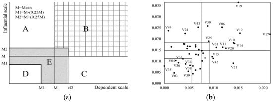
Figure 4. The influence-dependence chart. (a) The influence-dependence chart area of variables; and (b) the position of study variables on the influence-dependence chart.

(A) Input variables: These variables are highly influential and less dependent. They tend to describe the dynamics of the system and the conditions of the other variables. Because of this, they are the first choice when developing different scenarios and strategies. According to Figure 4b, agricultural development in Iran has three input variables: V44, V24, and V43. This means that in order to develop dynamic and sustainable agricultural development in Iran, we must manage disasters, organize farmers, and improve farmers’ knowledge, awareness, and skills. Pavelic et al. [44] and Das [39] showed that flood and drought management is very important for agricultural development in Thailand and India. Also, there are many studies that emphasize the importance of human resources and capital (including schooling, training, organizing, and skills) for agricultural development [4,16,45]. Undoubtedly, building the human capital of smallholder farmers can play a critical role in agricultural growth and development.

(B) Relay or intermediate variables: These variables are highly influential and highly dependent. Any change will have high flow throughout the rest variables of the system. Figure 4b demonstrates 11 relay variables for agricultural development in Iran. Among these variables V19 (government policies and programs), V17 (the amount of agricultural production), V12 (agricultural products price), and V06 (marketing) are the most important. Our findings were in line with various studies [11,42,46] in other areas.

(C) Resultant variables: These variables have a low degree of influence and are highly dependent. Result variables are influenced by both the input variables or determinants (A) and the relay variables (B). Based on Figure 4b, there are three resultant variables in Iran’s agriculture system. These are V15 (storage facilities), V21 (farmers’ interest and motivation), and V45 (crop insurance). Some studies, such as John and Samuel Noi [33] and Qingshui and Xuewei [22], have also noted the importance of these variables for agricultural development in other areas of the world.

(D) Excluded or independent variables: This group is relatively unconnected to the system. They only have a few relationships within it and are neither influential nor dependent variables. Due to their relatively autonomous character and lack of connection to the system, they are not determinants of the future of the system. Therefore, they can be excluded from the next steps of the analysis. As seen in Figure 4b, there are eight excluded variables (V03, V04, V34, V35, V36, V38, and V39) in our study.

(E) Average variables: These variables cannot be clearly allocated to the remaining sectors because they are not sufficiently influential or dependent. Though they should be recognized and studied more closely in the future. The remainder of the variables in this study belong to this group.

3.5. The Stability and Instability of Agricultural Development System

The pattern of distribution in Figure 4 can not only inform us about the various types of variables, but also presents the stability or instability of a system. The stability of an agricultural system is very important, because agriculture can play an important role in global stability [22,47]. This, then is very helpful to know and informs us about the stability of agriculture system. As Figure 5 shows, if the points are distributed around the main diagonal (see Figure 5a), then the system is unstable. But if the cloud of points is spread along the axis (as L shape: see Figure 5b), it means that the system is stable. The advantage of a stable system is that it introduces a dichotomy between the influential variables, on which one can or cannot act, and the resultant variables which depend on them [27,29]. Based on these explanations and as Figure 5c indicates, the agricultural development system in Iran is unstable. Each variable is both influential and dependent, and any action on one variable has repercussions on all the others and on the original variable. The instability of the Iranian agricultural system has also been highlighted by other studies [48] and in other areas [49,50,51,52].

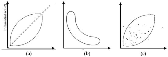
Figure 5. System stability according to the influence-dependence chart (a) Unstable system; (b) Stable system; and (c) Iran agricultural development system.

4. Conclusions

Agricultural systems, especially in developing countries, are typically complex, and when forming strategies and scenarios, available methods have failed to reveal the essence of such complex systems. Therefore, the main objective of this study was to address this problem by using an integrated method. We integrated the MICMAC and AHP methods, using the MICMAC to determine the various classifications of variables and the AHP method to apply weights to these different variables. The case of the agricultural system of Iran was used to indicate an application of this new integrated method. The results revealed that the various types of variables in agricultural systems, from “actual direct influence” to “potential indirect dependence”, did not present similar influences or dependencies on each other. As a result, the ranks of key variables may change by applying the weight of different classification types of variables. Additionally, the AHP-MICMAC method allows us to have a total priority for each variable that helps policy and decision makers to recognize the most important variable according to its dependency and influence on other variables.

For example, in the Iran case, based on the total priority scores of the strategic variables, “farmers’ organizing and institutionalizing”, “farmers’ knowledge, awareness, and skills”, and “disasters”, respectively, are three main variables that describe the conditions and the dynamics of the other variables of agricultural systems. Therefore, they have a critical role in agricultural growth and development. “Government policies and programs” is the most important intermediate variable for agricultural development. It means the instability of the policies and programs will have high flow throughout the rest variables of the system. “Farmers’ interest and motivation”, “storage facilities”, and “crop insurance” are three main highly dependent variables that are influenced by both input and intermediate variables. There also are some variables, such as “agricultural support system”, “water efficiency”, “agricultural research”, “pricing system”, “rural welfare and comforting”, “agricultural land area”, “transportation and communications”, and “trade incentives and restrictions”, that they should be recognized and studied more closely in the future.

According to expert opinion, the use of the AHP-MICMAC method has led to a more realistic ranking of the variables and this combination has been able to improve results. It then facilitates the ranking of the variables according to their different types of influences and dependency weights. Without a doubt, any improvement in our understanding of the key variables of a system will lead to forming better scenarios and strategies for development of that system. Although the AHP-MICMAC method is more capable of illustrating the complexities among the variables than many other current methods, it still needs to be developed further so that it can better reflect the interdependency of variables, including economic, social, environmental, religious, etc., which can lead to risky, diverse, and complex agriculture in developing countries, such as Iran. In this regard, performing a study in order to compare the effectiveness of various methods, such as system dynamic modeling, AHP-MICMAC, or cross-impact analysis to display these complexities, is very crucial.

References

- Zhao, S.; Li, P.; Xiong, Y.; Zhang, X.; Chai, L. Complex agricultural system evolution basing on fourth thermodynamic law. In Proceedings of the 2012 Eighth International Conference on Natural Computation (ICNC), Chongqing, China, 29–31 May 2012; pp. 20–24. [Google Scholar]
- Mudgal, R. Poverty Alleviation and Rural Development; Sarup & Sons.: New Delhi, India, 2006. [Google Scholar]
- Nesheim, M.C.; Oria, M.; Yih, P.T. A Framework for Assessing Effects of the Food System; National Academies Press: Washington, DC, USA, 2015. [Google Scholar]
- Ames, G.C.W. Human capital, agricultural development and the African food crisis. Agric. Adm. Ext. 1988, 28, 1–17. [Google Scholar] [CrossRef]
- Schreinemachers, P.; Berger, T. An agent-based simulation model of human–environment interactions in agricultural systems. Environ. Model. Softw. 2011, 26, 845–859. [Google Scholar] [CrossRef]
- Viaggi, D.; Raggi, M.; Gomez y Paloma, S. Modelling and interpreting the impact of policy and price scenarios on farm-household sustainability: Farming systems vs. result-driven clustering. Environ. Model. Softw. 2013, 43, 96–108. [Google Scholar] [CrossRef]
- Kusunose, Y.; Mahmood, R. Imperfect forecasts and decision making in agriculture. Agric. Syst. 2016, 146, 103–110. [Google Scholar] [CrossRef]
- Wang, J.; Chen, J.; Ju, W.; Li, M. IA-SDSS: A GIS-based land use decision support system with consideration of carbon sequestration. Environ. Model. Softw. 2010, 25, 539–553. [Google Scholar] [CrossRef]
- Balbi, S.; Prado, A.d.; Gallejones, P.; Geevan, C.P.; Pardo, G.; Pérez-Miñana, E.; Manrique, R.; Hernandez-Santiago, C.; Villa, F. Modeling trade-offs among ecosystem services in agricultural production systems. Environ. Model. Softw. 2015, 72, 314–326. [Google Scholar] [CrossRef]
- Archer, D.W.; Dawson, J.; Kreuter, U.P.; Hendrickson, M.; Halloran, J.M. Social and political influences on agricultural systems. Renew. Agric. Food Syst. 2008, 23, 272–284. [Google Scholar] [CrossRef]
- Schirmer, S. Market Regulation and Agricultural Development; Econometric Research Southern Africa, University of the Witwatersrand: Johannesburg, South Africa, 2001. [Google Scholar]
- Yanli, Z. An Introduction to the Development and Regulation of Agricultural Insurance in China. Geneva Pap. Risk Insur. Issues Pract. 2009, 34, 78–84. [Google Scholar]
- Pinstrup-Andersen, P.; Shimokawa, S. Rural Infrastructure and Agricultural Development; World Bank: Washington, DC, USA, 2006; Available online: http://siteresources.worldbank.org/INTDECABCTOK2006/Resources/Per_Pinstrup_Andersen_Rural_Infrastructure.pdf (accessed on 17 July 2019).
- Amadi, B.C. The impact of rural road construction on agricultural development: An empirical study of Anambra state in nigeria. Agric. Syst. 1988, 27, 1–9. [Google Scholar] [CrossRef]
- FAO. Improving Agricultural Extension: A Reference Manual; Swanson, B.E., Bentz, R.P., Sofranko, A.J., Eds.; FAO: Rome, Italy, 1997. [Google Scholar]
- Alexandratos, N.; Bruinsma, J. World Agriculture towards 2030/2050: The 2012 Revision; ESA Working paper; ESA: Rome, Italy, 2012. [Google Scholar]
- Rótolo, G.C.; Montico, S.; Francis, C.A.; Ulgiati, S. How land allocation and technology innovation affect the sustainability of agriculture in Argentina Pampas: An expanded life cycle analysis. Agric. Syst. 2015, 141, 79–93. [Google Scholar] [CrossRef]
- de Olde, E.M.; Moller, H.; Marchand, F.; McDowell, R.W.; MacLeod, C.J.; Sautier, M.; Halloy, S.; Barber, A.; Benge, J.; Bockstaller, C.; et al. When experts disagree: The need to rethink indicator selection for assessing sustainability of agriculture. Environ. Dev. Sustain. 2017, 19, 1327–1342. [Google Scholar] [CrossRef]
- Musakwa, W.J.E. Identifying land suitable for agricultural land reform using GIS-MCDA in South Africa. Dev. Sustain. 2018, 20, 2281–2299. [Google Scholar] [CrossRef]
- Pascucci, S.; de-Magistris, T. The effects of changing regional Agricultural Knowledge and Innovation System on Italian farmers’ strategies. Agric. Syst. 2011, 104, 746–754. [Google Scholar] [CrossRef]
- Allen, M.S. Bet-hedging strategies, agricultural change, and unpredictable environments: historical development of dryland agriculture in Kona, Hawaii. J. Anthropol. Archaeol. 2004, 23, 196–224. [Google Scholar] [CrossRef]
- Qingshui, F.; Xuewei, Z. Development Strategies on Agricultural Insurance under the Building of New Countryside. J. Agric. Sci. Tech. 2010, 1, 13–23. [Google Scholar] [CrossRef][Green Version]
- Zhou, Y.; Wang, X.; Cai, Y. Reasons and Improving Strategies of Slow Development of Agricultural Insurance System in China. J. Northeast Agric. Univ. (Engl. Ed.) 2011, 18, 92–96. [Google Scholar] [CrossRef]
- Villacorta, P.J.; Masegosa, A.D.; Castellanos, D.; Lamata, M.T. A linguistic approach to structural analysis in prospective studies. In Proceedings of the International Conference on Information Processing and Management of Uncertainty in Knowledge-Based Systems, Catania, Italy, 9–13 July 2012; pp. 150–159. [Google Scholar]
- Godet, M. The art of scenarios and strategic planning: tools and pitfalls. Technol. Forecast. Soc. Chang. 2000, 65, 3–22. [Google Scholar] [CrossRef]
- Saaty, T.L. Decision making with the analytic hierarchy process. Int. J. Serv. Sci. 2008, 1, 83–98. [Google Scholar] [CrossRef]
- Mirakyan, A.; De Guio, R. Three Domain Modelling and Uncertainty Analysis: Applications in Long Range Infrastructure Planning; Springer: Germany, Switzerland, 2015. [Google Scholar]
- Godet, M. Manuel of Strategic forecasting. Volume 2 (Manuel de Prospective Stratégique. Tome 2); Dunod: Berlin, France, 1997. [Google Scholar]
- Godet, M. From Anticipation to Action: A Handbook of Strategic Prospective; UNESCO Publishing: Dunod, Paris, 1994. [Google Scholar]
- Saaty, T.L. The analytic hierarchy and analytic network measurement processes: Applications to decisions under risk. Eur. J. Pure Appl. Math. 2007, 1, 122–196. [Google Scholar]
- Saaty, T.L. The Analytic Hierarchy Process; McGraw-Hill International: New York, NY, USA, 1980. [Google Scholar]
- Godet, M.; Durance, P. Strategic Foresight for Corporate and Regional Development; Unesco: Paris, France, 2011. [Google Scholar]
- John, B.-B.; Samuel Noi, A. The Effect of Government Policies on Agricultural Prices and Output in a Developing Country. J. Dev. Areas 1995, 30, 91–112. [Google Scholar]
- Norton, J.P.; Reckhow, K.H. Modelling and Monitoring Environmental Outcomes in Adaptive Management. In Developments in Integrated Environmental Assessment; Jakeman, A.J., Chen, S.H., Eds.; Elsevier: Amsterdam, The Netherlands, 2008; Volume 3, pp. 181–204. [Google Scholar]
- Bowman, M.S.; Zilberman, D. Economic Factors Affecting Diversified Farming Systems. Ecol. Soc. 2013, 18. [Google Scholar] [CrossRef]
- Van Velthuizen, H. Mapping Biophysical Factors that Influence Agricultural Production and Rural Vulnerability; Food and Agriculture Organization of the United Nations: Rome, Italy, 2007. [Google Scholar]
- World Bank. World Development Report 2008: Agriculture for Development; World Bank: Washington, DC, USA, 2007. [Google Scholar] [CrossRef]
- Mousavi, S.-F. Agricultural drought management in Iran. In Water Conservation, Reuse, and Recycling: Proceedings of an Iranian-American Workshop; National Academies Press: Washington, DC, USA; pp. 106–113.
- Das, H.P. Agricultural Drought Mitigation and Management of Sustained Agricultural Development in India. In Natural Disasters and Extreme Events in Agriculture: Impacts and Mitigation; Sivakumar, M.V.K., Motha, R.P., Das, H.P., Eds.; Springer: Berlin/Heidelberg, Germany, 2005; pp. 277–303. [Google Scholar] [CrossRef]
- Hazell, P.B.; Pomareda, C.; Valdes, A. Crop Insurance for Agricultural Development: Issues and Experience; IICA Biblioteca Venezuela: Caracas, Venezuela, 1986. [Google Scholar]
- Skees, J.; Hazell, P.B.; Miranda, M. New Approaches to Crop Yield Insurance in Developing Countries; International Food Policy Research Institute (IFPRI): Washington, DC, USA, 1999. [Google Scholar]
- Adigal, V.; Singh, S. Agricultural marketing vis-a-vis warehousing facility (Case study of Central Warehousing Corporation). Bus. Manag. Rev. 2015, 5, 43. [Google Scholar]
- Jouanjean, M.-A. Targeting Infrastructure Development to Foster Agricultural Trade and Market Integration in Developing Countries: An Analytical Review; Overseas Development Institute: London, UK, 2013. [Google Scholar]
- Pavelic, P.; Srisuk, K.; Saraphirom, P.; Nadee, S.; Pholkern, K.; Chusanathas, S.; Munyou, S.; Tangsutthinon, T.; Intarasut, T.; Smakhtin, V. Balancing-out floods and droughts: Opportunities to utilize floodwater harvesting and groundwater storage for agricultural development in Thailand. J. Hydrol. 2012, 470–471, 55–64. [Google Scholar] [CrossRef]
- Parman, J. Good schools make good neighbors: Human capital spillovers in early 20th century agriculture. Explor. Econ. Hist. 2012, 49, 316–334. [Google Scholar] [CrossRef]
- Akinbamowo, R. A review of government policy on agricultural mechanization in Nigeria. J. Agric. Ext. Rural Dev. 2013, 5, 146–153. [Google Scholar]
- Tilman, D.; Cassman, K.G.; Matson, P.A.; Naylor, R.; Polasky, S. Agricultural sustainability and intensive production practices. Nature 2002, 418, 671–677. [Google Scholar] [CrossRef]
- Karshenas, M. Oil, State and Industrialization in Iran; Cambridge University Press: Cambridge, UK, 1990. [Google Scholar]
- Hathaway, D.E. Agriculture in an Unstable Economy Revisited. J. Farm Econ. 1959, 41, 487–499. [Google Scholar] [CrossRef]
- ICARDA; FAO; AARINENA; CIHEAM. The National Agricultural Research Systems in the West Asia and North Africa Region; ICARDA: Aleppo, Syria, 1999; Volume vii. [Google Scholar]
- Sharma, M.; Dhiman, R. Agribusiness Strategies to Promote Exports: An Analysis of Growth and Instability. Int. J. Manag. Soc. Sci. 2015, 3, 622–637. [Google Scholar]
- Squires, V.R. The Role of Food, Agriculture, Forestry and Fisheries in Human Nutrition—Volume IV; EOLSS Publications: Paris, France, 2011. [Google Scholar]
© 2019 by the authors. Licensee MDPI, Basel, Switzerland. This article is an open access article distributed under the terms and conditions of the Creative Commons Attribution (CC BY) license (http://creativecommons.org/licenses/by/4.0/).