Nonlinear Relationships between Oil Prices and Implied Volatilities: Providing More Valuable Information

Abstract

This paper investigates the linear/nonlinear long-run and short-run dynamic relationships between oil prices and two implied volatilities, oil price volatility index (OVX) and stock index options volatility index (VIX), representing panic gauges. The results show that there is a long-run equilibrium relationship between oil prices and OVX (VIX) using the linear autoregressive distributed lag (ARDL)-bounds test. Likewise, while using the nonlinear autoregressive distributed lag (NARDL)-bounds test, not only does a long-run equilibrium relationship exist, but also the rising OVX (VIX) has a greater negative influence on oil prices than the declining OVX (VIX), thus indicating that a long-run, asymmetric cointegration exists between the variables. Furthermore, OVX (VIX) oil prices have a linear Granger causality, while for the nonlinear Granger causality test, oil prices have a bidirectional relation with OVX (VIX). In addition, we find that once major international political and economic events occur, structural changes in oil prices change the behavior of oil prices, and thus panic indices, thereby switching from a linear relationship to a nonlinear one. The empirical results of this study provide market participants with more valuable information.

1. Introduction

Dramatic fluctuations in oil prices have had a major impact on various commodity markets, especially the severe financial crisis in mid-September 2008 that led to structural changes in the crude oil market [1,2] making the system of the entire market more vulnerable. Oil market participants have become more sensitive to external information such as oil price or stock price volatility and may change their trading strategies.

The statement at the website [3] claims that the Chicago Board Options Exchange (CBOE) Crude Oil ETF Volatility Index (OVX) measures the market’s expectation of 30-day volatility of crude oil prices by applying the stock index options volatility index (VIX) methodology to United States Oil Fund, LP (USO) options spanning a wide range of strike prices. Although many studies have suggested that the performance of the volatility model can be significantly improved by including VIX [4], it is surprising that crude oil OVX did not attract much attention in predicting oil price changes. Because OVX is a market-determined forecast, it is very similar to the stock market’s implied volatility index [1]. For example, ref. [5] pointed out that OVX is a measure of uncertainty in the oil market and can directly predict market expectations for future 30-day crude oil price volatility. In ref. [6], the authors argued that since volatility comes from market option prices, these prices are forward-looking and, therefore, represent a market consensus on expected future uncertainties. Furthermore, in the literature on oil prices and related volatilities, authors in [7] indicated that oil price volatility positively influences stock returns, but the impact of implied volatility index of crude oil (OVX) is negative, which means the rise in future oil price uncertainty has caused the stock prices to fall. Using the implied volatility index (VIX) provided by Chicago Board Options Exchange (CBOE) to study the relationship between oil price and the US energy stock returns, authors in [8] showed that a long-run relationship exists between the oil and VIX. Also in the causality test, there was a short-run leading effect between the OVX and the US energy stock returns. Authors in [9] found that the lead–lag relation between the oil price and its volatility is central to any type of trading strategy based on futures and options on the OVX. Authors in [10] further pointed out that there is a negative and asymmetric relationship between OVX changes and crude oil price returns. Authors in [11] also documented that there is a significant, negative relationship between OVX changes and West Texas Intermediate (WTI) returns, and that the asymmetry relationship between them means the OVX has a greater predictive effect of gauging an investor’s fear rather than risk preference.

Furthermore, scholars in the economics and finance field have been very concerned about the issue of how oil price changes have been caused by structural changes in the crude oil market. Authors in [1] found that during the three different structural periods the main drivers of oil price changes had significantly different effects on them. After accounting for structural breaks in the generalized autoregressive conditional heteroskedasticity (GARCH) model, authors in [12] demonstrated that a strong volatility spillover effect exists between the oil price and the US stock market. Authors in [13] indicated that the oil price has a one-way, nonlinear Granger causal relation with the US dollar exchange rate, and the short-run US dollar exchange rate has a more significant, negative impact on oil prices. If the structural changes are ignored during the financial crisis, the volatilities of the oil price and the US dollar exchange rate can increase with a negative correlation between them. Authors in [14] found that oil prices are linearly co-integrated with OVX (VIX) during some sample periods. If structural changes during periods of economic recession are considered, only a one-way, linear Granger causality relationship exists between oil prices and these two volatilities.

Accurate prediction in the fluctuation magnitude and trend of oil prices by using updated economic data is considerably challenging for academics and industries who have adopted traditional linear models. Especially with structural changes, the fluctuation and speed of oil prices are more confusing. Authors in [14,15] indicated that linear models with structural changes may not be able to detect the cointegration relationship between oil price and its volatility. Authors in [16] studied the conditional volatility of oil spot prices and future prices in various GARCH models, and they found that the fractionally integrated generalized autoregressive conditionally heteroskedastic (FIGARCH) model significantly reduced the degree of volatility persistence during the adjustment period after structural changes occurred. Authors in [17] used a nonlinear cointegration model with thresholds and found that, due to endogenous structural changes, there was no long-run equilibrium linear relationship between oil and Indian stock markets, while the short-run Granger causality relation held during some subperiods. We, therefore, question whether the structural change in oil prices leads to nonlinear behavior.

For example, authors in [18] found a nonlinear interaction between the oil market and the stock market in the Middle East and North Africa in nonlinear and asymmetrical causality tests. Authors in [17] showed that the nonlinear relationship between the oil market and the Indian stock market was significant after the global financial crisis in 2008 based on the results of the nonlinear cointegration test. Authors in [19] used a nonlinear autoregressive distributed lag (ARDL) model with panel data to find that oil price changes asymmetrically affect the stock markets of oil exporting and importing countries. Authors in [20] reported that the implied volatility of gold and oil has a nonlinear, positive cointegrated relationship with the implied volatility of Indian stocks. Authors in [21] conducted a nonlinear Granger causality test and found that there was a bidirectional, nonlinear relationship between oil prices and gold prices, and the results of the nonlinear ARDL test revealed that a positive shock in oil prices had a more pronounced effect than negative shocks on gold prices.

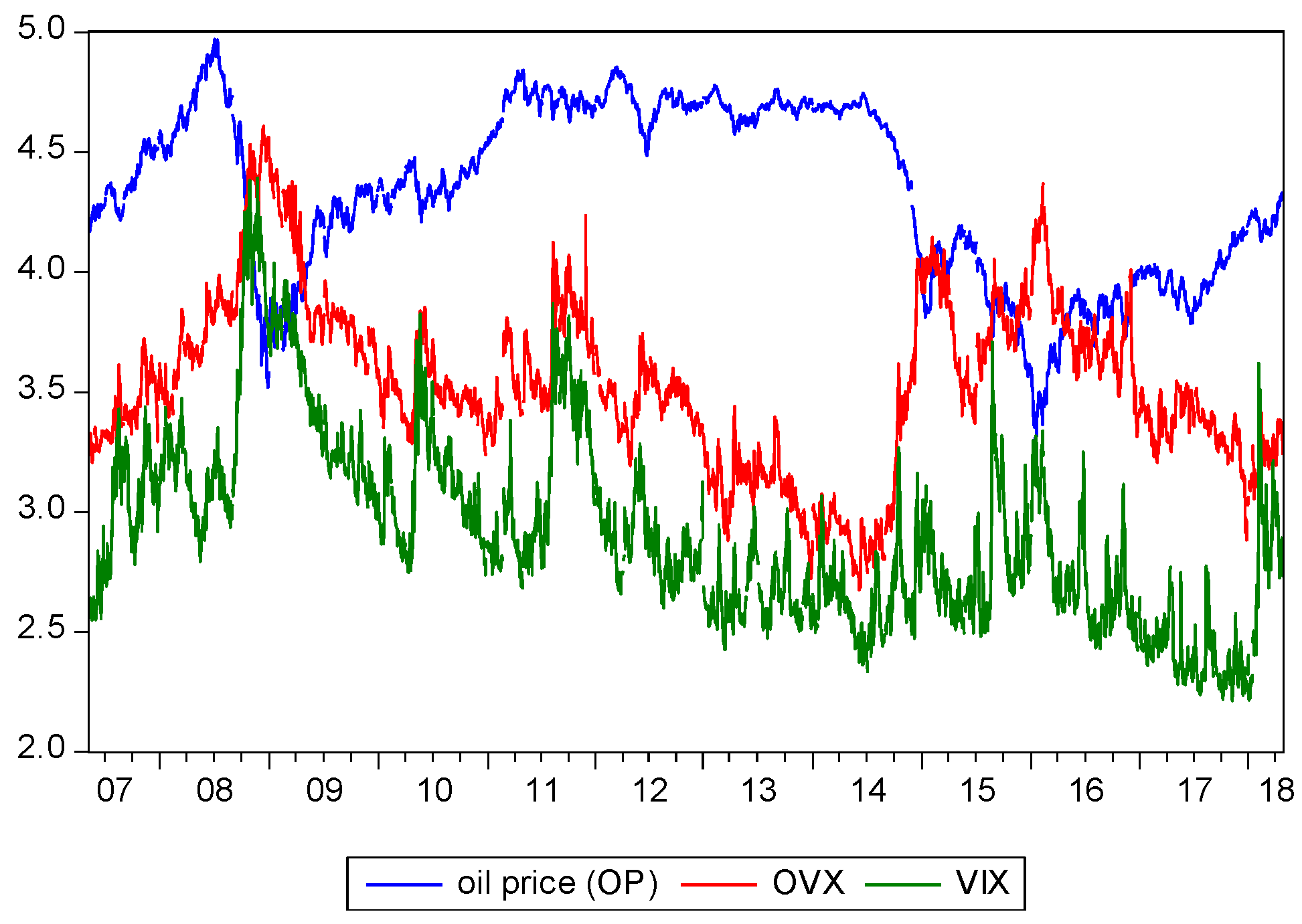
Straightforwardly, the literature on the nonlinear dynamic relationship between oil prices and its volatilities has lacked this kind of work. This paper aims to fill the gap in such a study. In other words, the purpose of this paper is to analyze the nonlinear long-run and short-run dynamic relationship between oil prices and its volatilities (VIX and OVX), representing the investor sentiment of stock and oil markets, to further understand how the structural change of oil prices, which might be caused by major international events, affect oil price behaviors.

Furthermore, in the short-run methodology, the linear Granger causality test may be unable to characterize the nature of nonlinear causality. Authors in [22] proposed a nonlinear Granger causality testing method (hereafter, HJ), but there was a problem of over-rejection of the null hypothesis in large samples. Authors in [23] modified the HJ model to effectively solve the shortcomings of large sample over-rejection (hereafter, DP). Since then, the DP model has been very popular in economics and finance fields [13,24,25,26,27]. On the other hand, in the long-run methodology, traditional cointegration methods, including Engle and [28,29], might have a problem with a weak testing power of the unit root if two series are not integrated on the same order. Authors in [30] therefore proposed the autoregressive distributed lag (ARDL) model to solve the problem of different integrated orders. However, this linear ARDL model still has the disadvantage of estimating bias when facing nonlinear relationships among variables. Authors in [31] proposed a nonlinear ARDL (NARDL) model to detect nonlinear long-run equilibrium relations among variables, which allows long-run and short-run asymmetry in testing variables and is robust to small samples [21]. Many related studies such as [21,32,33,34,35] all use this method in their empirical studies. Along with this reason, this paper adopts this method to examine the nonlinear long-run relationships between oil prices and two fear gauges (VIX and OVX).

The rest of the paper is organized as follows. Section 2 presents the methodology and data sources. Section 3 shows the empirical results and analysis. Finally, Section 4 concludes this paper.

2. Methodology and Data

2.1. Autoregressive Distributed Lag (ARDL) Models

A prerequisite for the ARDL test is to solve the problems that the mixture of different time series I(0) and I(1) present so there is no spurious regression, but it cannot be applicable for sequence I(2) or higher [5]. Before testing the ARDL model, the appropriate lag structure of the variables must be selected. We choose the model with the minimum Schwarz’s Bayesian information criterion (SBC), which was a maximum lag of 4. The linear ARDL model considered in the empirical analysis has the following form:

$$\Delta y_t=c_0+c_{1}t+{\pi }_1{y}_{t-1}+{\pi }_2{x}_{t-1}+{\displaystyle \sum }_{i=1}^p{\gamma }_i\Delta y_{t-i}+{\displaystyle \sum }_{j=1}^q{\delta }_j\Delta x_{t-j}+{\epsilon }_t$$

(1)

where y is the oil price, x is the oil price volatility index (OVX) or stock index options volatility index (VIX), $c_0$ is the intercept term, $c_1$ is the slope of the time trend term, ${\epsilon }_t$ is white noise, and p and q are the lag periods of the difference term of dependent and independent variables, respectively. The notation of the model structure is expressed in ARDL (p, q).

In order to examine whether a cointegrated relationship exists between the variables, F statistics were used to jointly test the null hypothesis of the absence of cointegration ${\mathrm{H}}_0:{\pi }_1={\pi }_2=0$ against the alternative hypothesis of the presence of cointegration ${\mathrm{H}}_0:{\pi }_1\ne {\pi }_2\ne 0$, while t statistics were used to test ${\mathrm{H}}_0:{\pi }_1=0$, the significance of the regressors. As [30] indicated, rejecting ${\mathrm{H}}_0:{\pi }_1={\pi }_2=0$ implies y_t and x_t have a long-run comovement relationship, which clearly states cointegration between the variables exists at the usual level of significance. If the independent variable is I (d) $(0\le d\le 1)$, the boundary between two asymptotic critical values provides the cointegration test, which assumes that the lower limit of the independent variable is I(0) and the upper limit is I(1). If the F value of the test statistic exceeds the upper limit, there will be long-term equilibrium cointegration between two variables; if the test statistic is lower than the lower limit, the null hypothesis of cointegration will be rejected, but if the test statistic is between the upper and lower limits, it will be impossible to make a judgment. For the mixed I(0) and I(1) case, the F statistics were calculated and compared with two different sets of critical values provided by [30].

Furthermore, if x and y have nonlinear relationships, the use of the ARDL approach is inappropriate. Authors in [31] proposed an extension of [30] to characterize the asymmetric property of two series. In line with [31], the nonlinear version of the ARDL (NARDL) approach can be defined as:

$$\Delta y_t=c_0+c_{1}t+{\pi }_1{y}_{t-1}+{\pi }_{21}{x}_{t-1}^{+}+{\pi }_{22}{x}_{t-1}^{-}+{\displaystyle \sum _{i=1}^p{\gamma }_i\Delta y_{t-1}+}{\displaystyle \sum _{j=1}^q({\delta }_{j1}\Delta x_{t-j}^{+}+}{\delta }_{j2}\Delta x_{t-j}^{-})+{\epsilon }_t,$$

(2)

where $x^{+}={\displaystyle \sum _{j=1}^q\Delta x_j^{+}}={\displaystyle \sum _{j=1}^q\max (\Delta x_j},0)$ and $x^{-}={\displaystyle \sum _{j=1}^q\Delta x_j^{-}}={\displaystyle \sum _{j=1}^q\min (\Delta x_j},0)$.

Rejecting $H_0:{\pi }_{21}={\pi }_{22}={\pi }_1=0$ means that cointegration exists between the variables. In addition, the parameters of the long-run asymmetric relationships can be measured as ${\theta }^{+}=-\frac{{\pi }_{21}}{{\pi }_1}$ and ${\theta }^{-}=-\frac{{\pi }_{22}}{{\pi }_1}.$

There are three strengths in using the ARDL test to analyze cointegration among variables. First, it is unnecessary to consider if the integration orders of variables are the same. Second, it can strengthen the test power of a small number of samples. Third, it is possible to identify dependent and independent variables themselves. However, there are two weaknesses regarding the use of the ARDL bounds test. As stated above, if the F value is between the upper limit and lower limit, it will be impossible to judge whether cointegration between variables exists. In addition, the use of this test is inappropriate if the time series data show nonlinear characteristics.

2.2. Nonlinear Granger Causality Test

Before studying nonlinearity, we first introduce linear causality. Authors in [36] introduced a causality test, and the basic concept of a Granger causality test is that future events will not have a causal effect on the present and the past. Past events can have an impact on the present and the future. Through this test, this paper examines whether there is mutual predictability between oil prices and OVX (VIX). The following bivariate (vector autoregressive, VAR) model is estimated based on the error correction method:

$$\Delta x_t={\alpha }_0+{\displaystyle \sum _{i=1}^p{\alpha }_{1,i}\Delta y_{t-i}+}{\displaystyle \sum _{j=1}^p{\alpha }_{2,i}\Delta x_{t-i}+}{\alpha }_{3}ec{t}_{t-1}+{\epsilon }_{1t};$$

(3)

$$\Delta y_t={\beta }_0+{\displaystyle \sum _{i=1}^p{\beta }_{1,i}\Delta x_{t-i}+}{\displaystyle \sum _{j=1}^p{\beta }_{2,i}\Delta y_{t-j}+}{\beta }_{3}ec{t}_{t-1}+{\epsilon }_{2t};$$

(4)

where $ec{t}_{t-1}$ is a one-period lag correction error term, and the other notations are as defined above. In (3), the Granger causality method tests $H_0:{\alpha }_1=0$, indicating that if the null hypothesis is accepted, $y_t$ does not exist a linear Granger causality with $x_t$. Similarly, in (4), the null $H_0:{\beta }_1=0$ is accepted, implying that $x_t$ does not have a linear Granger causality with $y_t$.

However, based upon the fact that the linear Granger causality method does not take into account the nonlinear causality between variables, we used the nonlinear Granger causality approach proposed by [23].

For two sets of strictly stationary time series, $x_t$ and $y_t$, if $x_{t-i}$ and $x_t$ contain additional information about $y_{t+j}$, then $x_t$ can strictly have a Granger causality with $y_t$. Let $F_{x,t}$ and $F_{y,t}$ denote the set of past observations containing $x_t$ and $y_t$ prior to $t+1$, respectively. Let ~ represent the equivalence of the distribution. The time series $x_t$ can strictly have a Granger causality with y_t when the following conditions are satisfied:

$$(y_{t+1,\dots ,}{y}_{t+n})|(F_{x,t},F_{y,t})\sim (y_{t+1,\dots ,}{y}_{t+n})|F_{x,t},$$

(5)

where n ≥ 1 represents the boundary of the prediction. When n = 1, the conditional distribution is compared with and without $y_t$ and $x_{t-i}$. Suppose the lag vector matrices $x_t^{lx}=(x_{t-lx+1},\dots ,x_t)$ and $y_t^{ly}=(y_{t-ly+1},\dots ,y_t)$, $(l_x,l_y\ge 1)$; the null hypothesis is that $x_t^{lx}$ does not contain any information that can predict $y_t^{ly}$, as follows:

$$H_0:y_{t+1}|(x_t^{lx};y_t^{ly})\sim y_{t+1}|y_t^{ly}.$$

(6)

For a strictly stationary bivariate time series, (6) indicates that the distribution of the $(l_x+l_y+1)$ dimensional vector $v_t=(x_t^{lx},y^{ly},z_t)$ will remain unchanged, where $z_t=y_{t+1}$. For the sake of simplicity, the time subscript is removed and $(l_x+l_y=1)$ is assumed. Then, the conditional distribution of z, given $(x,y)=(x^{*},y^{*})$, is the same as that of z given $(x,y)=(x^{*},y^{*})$. Thus, (6) can be rewritten by the joint probability density function in the following way:

$$\frac{f_{x,y,z}(x^{*},y^{*},z^{*})}{f_y(y^{*})}=\frac{f_{x,y}(x^{*},y^{*})}{f_y(y^{*})}.\frac{f_{x,z}(x^{*},z^{*})}{f_y(y^{*})}.$$

(7)

In terms of (7), x and z are conditional and independent of y = y^* for each y^*, so the modified H₀ indicates that the following relation is established:

$$G\equiv E[f_{x,y,z}(x,y,z)f_y(y)-f_{x,y}(x,y)f_{y,z}(y,z)]=0.$$

(8)

Let $\widehat{f_v}(v_i)$ denote the local density function estimated value of the random vector $v$ at $v_i$, as follows:

$$\widehat{f_v}(v_i)=\frac{{(2{\mu }_m)}^{-dv}}{(n-1)}{\displaystyle \sum _{j,j\ne i}{I}_{ij}^v},$$

(9)

where $I_{ij}^v=I(||v_i-v_j||<{\mu }_m),I(\cdot )$ is the index function, and μ_m is the bandwidth parameter associated with the number of samples $(m)$. When a local density function is estimated, we obtain the following test statistic:

$$T_m({\mu }_m)=\frac{m-1}{m(m-2)}.{\displaystyle \sum _i[({\widehat{f}}_{x,y,z}{x}_i,y_i,x_i){\widehat{f}}_y(y_i)-{\widehat{f}}_{x,y}(x_i,y_i){\widehat{f}}_{y,z}(x_i,z_i)}].$$

(10)

For $l_x+l_y=1$, and if we let the bandwidth depend on the sample size as:

$${\mu }_m=C{m}_{}^{-\beta },$$

(11)

where $0<C$ and $\frac{1}{4}<\beta <\frac{1}{3}$, then the statistic $T_m({\mu }_m)$ satisfies the following condition:

$$\sqrt{m}\frac{(T_m({\mu }_m)-G}{S_m}\stackrel{\hspace{1em}d\hspace{1em}}{\to }N(0,1),$$

(12)

where $\stackrel{\hspace{1em}d\hspace{1em}}{\to }$ denotes the distribution convergence, and $S_m$ denotes the estimated value of the asymptotic variance of $T_m(\cdot )$.

2.3. Data

In this study, the data sources were from Federal Reserve Economic Data, (FRED), which covered 2750 observations over 10 May 2007 to 22 April 2018. For studying convenience, all the variables surveyed were in natural logarithm, and Eviews 9.0 was used as the analysis software for this study [37]. The time series graphs for Brent oil price (OP), OVX, and VIX are shown in Figure 1.

3. Empirical Result and Analysis

3.1. Unit Root Test Results

In order to avoid spurious regression problems of the time series of all variables, we used the ADF test [38], PP test [39], and KPSS test [40]. The unit root testing results are that the series of oil price (OP) exhibits I (1), and those of OVX and VIX exhibit I (0). The results are shown in

Table 1. Results of Unit Root tests.

Level	ADF	PP	KPSS
OP	−1.598	−1.655	1.843 ***
OVX	−3.046 **	−2.903 **	0.068
VIX	−4.452 ***	−4.305 ***	0.072

Note: ** denotes significance at the 5% level, and *** denotes significance at the 1% level.

.

3.2. Results of the ARDL Test

Since oil price, OVX, and VIX are on different integrated orders, we used linear ARDL to study the impact of OVX and VIX on the oil price. Schwarz’s Bayesian information criterion (SBC) was more suitable to use in this study because of the large sample size used, and the optimal lag period was set to 2. The ARDL results are shown in

Table 2. Results of linear autoregressive distributed lag (ARDL) and ARDL bound test.

OVX ⟶ OP			VIX ⟶ OP
Variable	Coefficient	t-stat	Variable	Coefficient	t-stat
Constant	0.05 ***	4.026	Constant	0.042 ***	4.370
$O{P}_{t-1}$	0.993 ***	600.772	$O{P}_{t-1}$	0.995 ***	744.150
$OVX$	−0.118 ***	−14.183	$VIX$	−0.057 ***	−10.647
$OV{X}_{t-1}^{}$	0.071 ***	6.382	$VI{X}_{t-1}^{+}$	0.213 ***	2.962
$OV{X}_{t-2}^{}$	0.042 ***	4.935	$VI{X}_{t-2}^{+}$	0.029 ***	5.492
$L_{OVX}^{}$	−0.973 ***	−4.668	$L_{VIX}^{}$	−1.460 ***	−3.335
ECM(−1)	−0.006 ***	−3.717	ECM(−1)	−0.004 ***	−3.257
B.T Trend	8.037 **		B.T Trend	10.106 ***
$Ad{j}_{.}{R}^2$	0.996		$Ad{j}_{.}{R}^2$	0.996

Notes: 1. The upper-bound critical values are 6.26, 7.3, and 9.63 for 10%, 5%, and 1%; *, **, and *** represent significance at 10%, 5%, and 1% levels, respectively; B.T _Trend indicates that the bound test model has a linear trend term.

, which revealed that the oil price was simultaneously negatively impacted by OVX and VIX, but it was positively affected by one-period and two-period lags for OVX and VIX, respectively (The results of residuals with no autocorrelation before the ARDL model are examined. The Breusch–Godfrey serial correlation LM test showed that the F-statistic is 0.1404, and the Durbin–Watson statistic is 1.9998). This implies that the oil market has started to accumulate momentum in drastically changing oil prices for a major event that would perhaps happen in the near future, thereby leading to the rise (decrease) of OVX and VIX that causes the rise (decrease) of oil prices. However, on the day of the real major event, short-run speculators sold (bought) the oil spot in the opposite direction, thus causing the oil price to fall (rise). This phenomenon is very similar to the short-run trading of the stock spot market.

However, for the estimation of the long-run equilibrium relationship, the lower portion of Table 2 shows that the oil price was significantly, negatively related to the long-run OVX ($L_{OVX}^{}$) and VIX ($L_{VIX}^{}$). The estimated long-run coefficient is −0.973, which means that a 1% decline (rise) in the L_OVX leads to a 0.973% increase (decrease) in oil prices, while the estimated long-run coefficient is –1.46, which says that a 1% decline (rise) in the $L_{VIX}^{}$ leads to a 1.46% increase (decrease) in oil prices. Obviously, the change in oil price was more negatively impacted by $L_{VIX}^{}$ than $L_{OVX}^{}$. Moreover, since the oil price was cointegrated with OVX and VIX (at the 5% level), respectively, the short-run error correction coefficient of OVX representing the adjustment toward long-run equilibrium was larger than that of VIX, which were −0.006 and −0.004, respectively.

3.3. Linear Granger Causality Tests

In order to test for the short-run linear causal relationship between the table oil price and OVX (VIX), we applied the linear Granger causality test based on the linear VAR model. In

Table 3. Results of the linear Granger causality between OP, OVX, and VIX.

Causality Direction	F-Statistic	Causality Direction	F-Statistic	Optimal Lag
OP→OVX	1.884	OVX→OP	11.637 ***	2
OP→VIX	0.113	VIX→OP	24.780 ***	2

Notes: 1. ***, **, and * Represent at 1%, 5%, and 10%, respectively. 2. The optimal lag period is determined based on SBC.

, the results of the linear Granger causality test show that the null hypothesis, that the oil price does not have a Granger causality with OVX (VIX), was not rejected, with the insignificant F value being 1.884 (0.113). Nevertheless, OVX (VIX) has a Granger causality with the oil price, with an F value of 11.637 (24.780). Therefore, we can conclude that under the linear VAR framework, OVX (VIX) can be used to predict the volatility of the oil price in a one-way direction.

3.4. Brock–Dechert–Scheinkma (BDS) Test Results

The oil price may have a nonlinear relationship with OVX (VIX) due to structural changes in the oil price. If there is no further detection of whether there is a nonlinear relationship between them, estimation results would produce estimation bias because nonlinear relationship information would be neglected [11].

Here, we chose to use the nonlinearity Brock–Dechert–Scheinkma (hereafter BDS) approach proposed by [41] to detect the VAR residuals obtained by Equations (1) and (2). The null hypothesis in the BDS test with independent and identical distribution was rejected, which means that the time series had nonlinear characteristics under different dimensions (m = 2, 3, ..., 6). As shown in

Table 4. Results of Brock–Dechert–Scheinkma (BDS) statistics from VAR residuals.

Dimension	BDS Statistic
	OP	OVX	VIX
2	0.0157 *** (0.00)	0.0143 *** (0.00)	0.0112 *** (0.00)
3	0.0343 *** (0.00)	0.0258 *** (0.00)	0.0284 *** (0.00)
4	0.0484 *** (0.00)	0.0324 *** (0.00)	0.0408 *** (0.00)
5	0.0593 *** (0.00)	0.0353 *** (0.00)	0.0470 *** (0.00)
6	0.0649 *** (0.00)	0.0357 *** (0.00)	0.0484 *** (0.00)

Note: 1. Figures in the parenthesis are p-values. The sample period is from 10 May 2007 to 28 April 2018. 2. *** indicates the significance of nonlinear dependency at the 1% level.

, the BDS test results show that the null hypothesis of linear dependence was rejected at the 1% level, thus indicating that the nonlinear Granger causality model was more suitable for detecting the short-run relationship between the oil price and OVX (VIX) than the linear model.

3.5. Results of Structural Breaks

Next, we wanted to detect whether the structural change problems existed with oil prices due to major international events so that we could further confirm if the oil price behavior had nonlinear characteristics. Referring to the structural change issue, authors in [42] and [43] suggested that the possible locations of change points should be confirmed before the model is set. The unit root test by [44] would cause problems in confining given points under structural changes. Authors in [45] tried converting the unit root test of structural change of given points into the unit root test on unknown points to allow the estimation of the locations of structural change points. Authors in [46] considered time points of structural change that were endogenously determined by the model itself. Authors in [47] solved the problem of identifying given change points, but only a single structural change point could be obtained, which led to a reduction of the testing power for time series data under multiple structural changes. Authors in [48] and [49] proposed a modified technique to find the mean and trends of multiple structural change points. But the empirical study by [50] showed that the method by [49] could be used to effectively find out structural change points. Authors in [51] pointed out that many major events would have various impacts on overall economic variables, thus they developed a unit root test that extended the structural change of an unknown point to the structural change of two unknown points.

Based on this reasoning, we used the multiple structural breaks approach proposed by [52] (Here, we used the Global L breaks vs. none method under the Bai and Perron (BP) model to detect structural changes in oil prices. Please see [52]). As shown in

Table 5. Results of structural breaks.

Parameter: Zt = [1]; q = 1; p = 1; M = 5; h = 15
Structural Break		Break
1	4.221 ***	29 December 2008
2	4.704 ***	1 December 2010
3	4.645 ***	4 April 2013
4	3.862 ***	3 December 2014
5	4.010 ***	2 September 2016
Adjusted R 2: 0.75 F-statistic: 1675.950 (0.00)

Note: 1. Global L breaks vs. none method on Eviews 9 is used in Table 5; 2. In the BP (1998) model, Zt = the number of independent variables, p = the number of lag periods of the dependent variable difference term, q = the number of lag periods of the independent variable difference term, M = the number of structural breaks, and h is the trimming percentage.

, there were five structural breaks caused by several major international political and economic events during the sampling period. The process of structural change concerning oil prices is described briefly in Figure 2 as follows. The first break was that in December 2008, due to the widespread global financial crisis, oil prices fell to the lowest price since 2004. Then, followed by the second break, the pressure of dollar depreciation since the implementation of QE2 in December 2010 gradually increased, and tremendous dollar funds evacuated from the US into the speculative markets of crude oil [53] making oil prices to rise to a new high since the financial tsunami. In April 2013, the third break occurred where the United States launched automatic spending cuts, which severely challenged economic recovery. The IMF’s revised global economic growth rate in 2013 and the weak economic data in China and the US all indicated that the global economic outlook remained fragile. At the fourth break in December 2014, the European Central Bank conducted a number of easing policies, the issue of independence in Scotland strengthened the US dollar, and the oil price fell even more [54]. Afterward, the prices of the three major international oil price indicators fell to a level below US $100 per barrel. The OPEC has once again maintained its production target and, thus, stimulated a major decline in international oil prices. In January 2016, the results of the OPEC semiannual meeting revealed that the oil-producing countries lacked a consensus on production, and the US announced that it would abolish the crude oil embargo, which caused the international oil market to seriously worry about its oversupply problem, further dragging down oil prices and touching a new low level ($26) since the tsunami. In September 2016, it slowly rebounded slightly above the fifth break, a recently crucial point ($45). We can see that there were major events before and after every structural breaking point, which caused the oil price to rise or fall sharply.

3.6. Nonlinear Autoregressive Distributed Lag (NARDL)-Bound Test Results

After confirming that the oil price was nonlinearly related to OVX (VIX), we further studied the asymmetric effects of OVX (VIX) on the oil price. First, the NARDL bound test results are shown in

Table 6. Nonlinear autoregressive distributed lag (NARDL) estimation results.

Panel A			Panel B
OVX $\stackrel{\mathit{N}\mathit{A}\mathit{R}\mathit{D}\mathit{L}}{\to }$ OP			VIX $\stackrel{\mathit{N}\mathit{A}\mathit{R}\mathit{D}\mathit{L}}{\to }$ OP
Variable	Coefficient	t-stat	Variable	Coefficient	t-stat
Constant	0.031 ***	3.809	Constant	0.025 ***	3.611
OPt−1	0.994 ***	596.254	OPt−1	0.997 ***	731.262
$OV{X}^{+}$	−0.126 ***	−9.646	$VI{X}^{+}$	−0.071 ***	−8.451
$OV{X}^{+}$	0.067 ***	3.552	$VI{X}_{t-1}^{+}$	0.028 ***	2.315
$OV{X}_{t-2}^{+}$	0.052 ***	4.126	$VI{X}_{t-2}^{+}$	0.038 ***	4.660
$OV{X}^{-}$	−0.107 ***	−6.550	$VI{X}^{-}$	−0.036 ***	−3.237
$OV{X}_{t-1}^{-}$	0.101 ***	6.269	$VI{X}_{t-1}^{-}$	0.031 ***	2.885
$L_{OVX}^{+}$	−0.919 ***	−4.340	$L_{VIX}^{+}$	−1.147 ***	−2.847
$L_{OVX}^{-}$	−0.900 ***	−4.281	$L_{VIX}^{-}$	−1.125 ***	−2.827
B.T Level	5.61 *		B.T Level	4.27 *
ECM(−1)	−0.006 ***	−3.577	ECM(−1)	−0.004 ***	−3.053
$W_{LR}$	5.281 ***	[0.00]	$W_{LR}$	4.678 **	[0.00]
$W_{SR}$	28.111 ***	[0.00]	$W_{SR}$	8.082 ***	[0.00]
$Ad{j}_{.}{R}^2$	0.996		$Ad{j}_{.}{R}^2$	0.996

Note: 1. The superscripts “+” and “−” show the positive and negative cumulative sums, respectively. 2. $L_{OVX}^{+}$, $L_{OVX}^{-}$ and $L_{VIX}^{+}$, and $L_{VIX}^{-}$ are the estimated long-run coefficients associated with positive and negative changes in oil prices. 3. *, **, and *** represent significance at 10%, 5%, and 1% levels, respectively.

(row 13). The F statistic of OVX (VIX), 5.61 (4.27), was significant, indicating that the oil price was nonlinearly cointegrated with OVX (VIX).

Then, by the Wald test, we can see the short-run and long-run asymmetry estimates of oil prices and OVX (VIX), in Table 6 (row 15), which indicated that the Wald statistic of OVX (VIX) in terms of a long-run relationship, W_LR, rejected the null hypothesis of long-run symmetric fluctuations in the oil price. With an estimated long-run coefficient of −0.919 (−0.900), there was a significant, long-run negative relationship between the oil price and a rise in OVX, $L_{OVX}^{+}$ and a decline in OVX, $L_{OVX}^{-}$, thereby indicating that an increase of 1% in OVX results in a 0.919% decline in the oil price, and a 1% decrease in OVX causes oil prices to rise by 0.9%. At the same time, there was also a significant, long-run negative relationship between the oil price and a rise in VIX, $L_{VIX}^{+}$ and a decline in VIX, $L_{VIX}^{-}$ with the estimated long-run coefficients being −1.147 and −1.125, respectively, This indicates that a 1% increase in VIX leads to a 1.147% decline in the oil price, while a 1% decline in VIX leads to a 1.125% increase in oil prices.

It is worthy to note that, in terms of short-run dynamic relationships (Table 6, row 1–10, 16), the Wald statistic (W_SR) of OVX (VIX) rejected the null hypothesis of symmetric fluctuations. This means that when OVX (VIX) rises, current OVX (VIX) negatively impacts the oil price, but one-period lag and two-period lag OVX (VIX) positively impact the oil price; when OVX (VIX) declines, current OVX (VIX) negatively impacts the oil price, but only one-period lag OVX (VIX) positively impacts the oil price (Table 6, row 9–10). However, in the long-run equilibrium analysis (Table 6, row 11–12), OVX (VIX) negatively impacts the oil price regardless of rising OVX (VIX) or declining OVX (VIX), but the impact of rising OVX (VIX) on the oil price is slightly greater than the impact of their decline on the oil price, which emphasizes a long-run, asymmetric co-integration between them.

3.7. Nonlinear Granger Causality Result

Since the oil price and OVX (VIX) have a nonlinear relationship, an analysis using the linear Granger causality test will probably lead to estimation bias as [15] indicated. In the following, this study will shift to the nonlinear Granger causal relationship between the oil price and OVX (VIX).

With the residual sequence previously obtained by the VAR model, the nonlinear relationships between relevant variables were confirmed by BDS and NARDL. Then, the nonlinear linkage mechanism between the variables was analyzed. According to the model in [23], parameters such as maximum lag (l), bandwidth parameter (C), theoretical optimization (β), and optimal bandwidth (${\mu }_m$) should be set to $l_x=l_y$ = 1, 2, 3, C = 6.75, $\beta$= 2/7, and ${\mu }_m$= 1.5, respectively. It should be noted here that l is the optimum lag in the linear model +1. (The parameters (C, $\beta$, and ${\mu }_m$) of the DP model are set and calculated from Equations (11,12). ${\mu }_m$ depends on the sample of the data and is equal to Max(Cm^-2/7, 1.5) based on the DP(2006) model).

Table 7. Results of nonlinear Granger causalities between oil prices and OVX (VIX).

lx = ly	H0: OP Does Not Cause VIX	H0: OVX Does Not Cause OP	H0: OP Does Not Cause VIX	H0: VIX Does Not Cause OP
	t-value	t-value	t-value	t-value
1	2.642 ***	2.450 ***	1.707 **	2.376 ***
2	3.700 ***	4.092 ***	2.365 ***	2.212 ***
3	3.212 ***	1.708 **	1.792 ***	1.090

Note: *, **, and *** denote that the null hypothesis is rejected at the 10%, 5%, and 1% significance levels, respectively.

shows the results of the nonlinear Granger causal relationship between the oil price and OVX (VIX). It is clear that there was bidirectional causality between the oil price and OVX in dimensions lx = ly = 1, 2, and 3, though that for VIX was simply in lx = ly = 1, 2. Apparently, the nonlinear causality results in Table 7 are rather different from the linear causality results in Table 3. In order to compare the difference between these two methods (linear vs. nonlinear Granger causality), we put the results together in the same table (

Table 8. Linear and nonlinear Granger causality between oil prices and OVX (VIX).

Linear Granger Causality	Results	Nonlinear Granger Causality	Results
H0: OP does not cause OVX	✕	H0: OP does not cause OVX	✓
H0: OVX does not cause OP	✓	H0: OVX does not cause OP	✓
H0: OP does not cause VIX	✕	H0: OP does not cause VIX	✓
H0: VIX does not cause OP	✓	H0: VIX does not cause OP	✓

Note 1. ✓represents H₀ is rejected, ✕ represents H₀ is accepted. 2. The use of significance levels in Table 8 is the same as in Table 3 and Table 7.

), where we will analyze their causal relationships in some detail.

In Table 8, we find that there was Granger causality between OVX (VIX) and the oil price in both the linear or nonlinear tests, while strong evidence supported bidirectional causality between the oil price and OVX (VIX) only in the nonlinear test. One plausible explanation is that there were structural changes in long-run oil prices caused by some major political and economic events, thereby resulting in complicated factors affecting the expectations of the oil market and stock market participants. One interesting work by [55] found that per capita GDP and health care expenditure of 20 middle–high-income countries had linear and nonlinear causal relationships. Recently, more studies relating to nonlinear causality, refer to [13,56,57,58], pointed out that nonlinear relations held between relevant variables.

The empirical results of the NARDL and nonlinear bidirectional causality between the oil price and OVX (VIX) in this study provide several important implications for the oil market and stock market participants. First, regardless of rising oil prices or declining oil prices, the two panic gauges, OVX and VIX, have long-run negative and asymmetric influences on the oil price, implying that, in terms of the change in oil prices, investors can use this negative relationship to predict long-run oil price movements. Second, investors can use the causal relationship between the oil price and the panic gauges to predict short-run (1–2 days) changes in oil prices; that is, previous (1–2 days) information concerning the two panic gauges positively impacts oil prices, but current information negatively impacts prices. Third, impacted by major political or economic events, a decline in the two panic gauges has a more significant influence on oil prices than a rise in the two gauges. Finally, gasoline suppliers importing a great quantity of oil from abroad can circumvent dramatic oil price impacts by buying longer-term contracts or options when the prices are in the lower levels.

4. Discussion

This paper employed a linear/nonlinear ARDL-bounds test to characterize the long-run cointegration of oil prices with two implied volatilities (OVX and VIX), representing panic gauges, and the short-run linear/nonlinear Granger causality between them. The results showed that the linear ARDL-bounds test method can only detect a long-run equilibrium relationship, while the NARDL-bounds test not only detected the long-run equilibrium relationship between oil price and OVX (VIX) but also found that the rising OVX (VIX) had a greater negative influence on the oil price than the declining OVX (VIX), thus indicating that a long-run, asymmetric cointegration exists between them. The results of linear Granger causality found that OVX (VIX) led the oil price in one direction. However, the nonlinear Granger causality test results showed that the oil price had a bidirectional nonlinear causality with OVX (VIX). Similarly, [21] showed strong evidence of a bidirectional, nonlinear relation between oil and gold prices. The nonlinearity and asymmetry of the interactive mechanism between oil and gold prices was also shown by using the nonlinear Granger causality test from [22]. Authors in [59] indicated the presence of cointegration relationships, a nonlinear and positive impact of the implied volatilities, and an inverse bidirectional causality between gold and oil on the implied volatility of the Indian stock market. Authors in [32] further found that the nonlinear ARDL models successfully captured the long-term linkages between oil and precious metal markets, and a bidirectional and symmetric effect presented between crude oil and gold markets using the nonlinear Granger causality test.

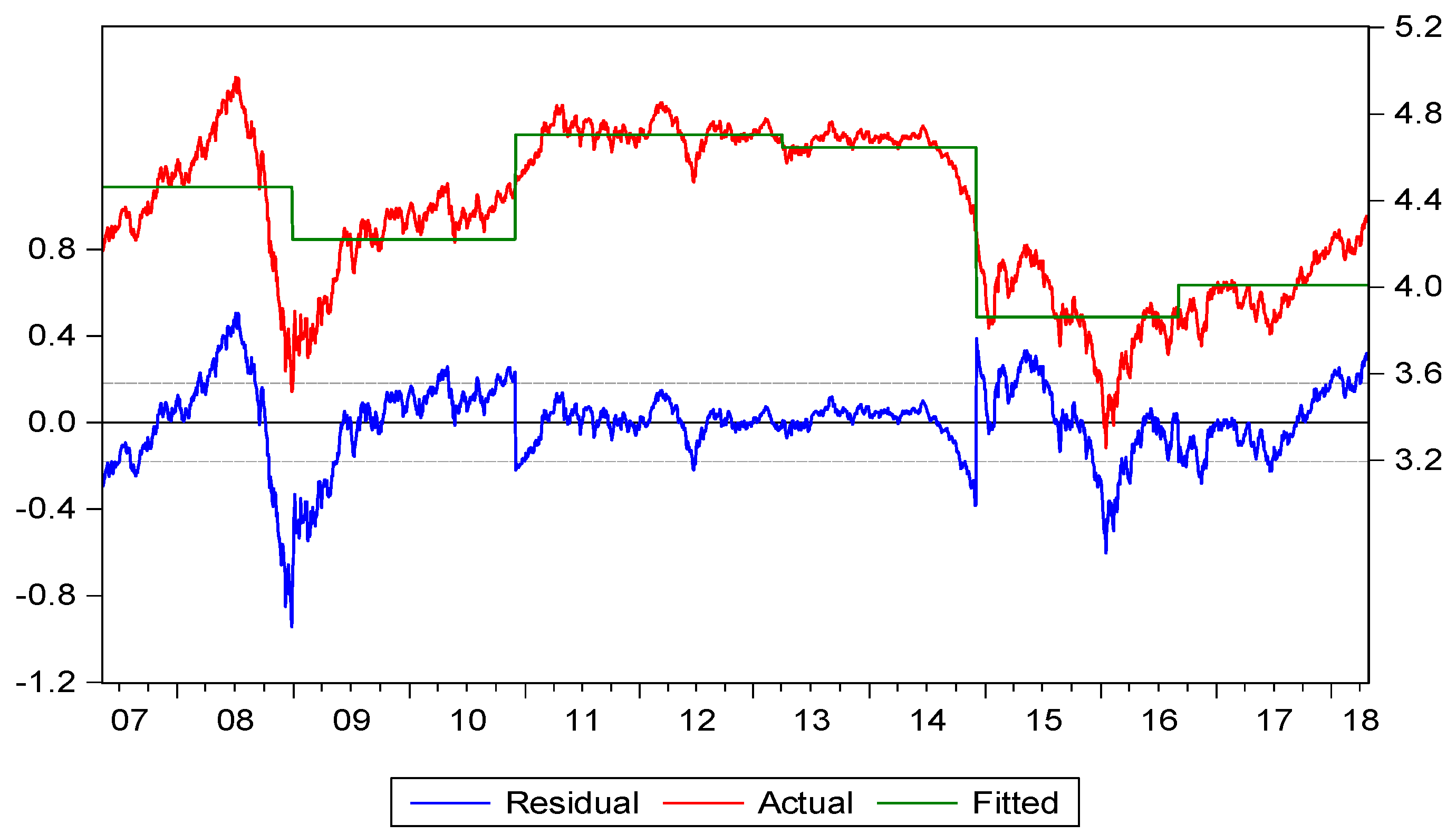
Meanwhile, we also saw that when major international political and economic events occur, such as government policies, geopolitical risks, investor sentiments, and natural disasters, structural changes in oil prices would change the behavior of oil prices and, thus, panic indices, which switched from a linear relationship to a nonlinear one. Therefore, the empirical results of this study investigating the long-run and short-run nonlinear relationships between oil prices and the two implied volatilities provide market participants with more valuable information (Recently, the nature of the nonlinear relationships between crude oil prices and other variables has led to increased interest in multiscale modelling approaches such as mode decomposition techniques (EMD). The interested readers may refer to the original paper of [60,61,62]).

References

1. Fan, Y.; Xu, J.-H. What has driven oil prices since 2000? A structural change perspective. Energy Econ. 2011, 33, 1082–1094. [Google Scholar] [CrossRef]
2. Ji, Q.; Fan, Y. How does oil price volatility affect non-energy commodity markets? Appl. Energy 2012, 89, 273–280. [Google Scholar] [CrossRef]
3. CBOE (Cboe Global Markets, Inc.). CBOE. Available online: www.cboe.com/OVX (accessed on 10 July 2019).
4. Taylor, S.J. Modelling Financial Time Series; World Scientific: Singapore, 2008. [Google Scholar]
5. Liu, M.-L.; Ji, Q.; Fan, Y. How does oil market uncertainty interact with other markets? An empirical analysis of implied volatility index. Energy 2013, 55, 860–868. [Google Scholar] [CrossRef]
6. Maghyereh, A.I.; Awartani, B.; Bouri, E. The directional volatility connectedness between crude oil and equity markets: New evidence from implied volatility indexes. Energy Econ. 2016, 57, 78–93. [Google Scholar] [CrossRef] [Green Version]
7. Vu, T.N. Impact of Crude Oil Volatility on Stock Returns: Evidence from Southeast Asian Markets; Vaasan yliopisto: Vaasa, Finland, 2018. [Google Scholar]
8. Dutta, A. Oil and energy sector stock markets: An analysis of implied volatility indexes. J. Multinatl. Financ. Manag. 2018, 44, 61–68. [Google Scholar] [CrossRef]
9. Aboura, S.; Chevallier, J. Leverage vs. feedback: Which Effect drives the oil market? Financ. Res. Lett. 2013, 10, 131–141. [Google Scholar] [CrossRef] [Green Version]
10. Chen, Y.; Zou, Y. Examination on the relationship between OVX and crude oil price with Kalman filter. Procedia Comput. Sci. 2015, 55, 1359–1365. [Google Scholar] [CrossRef]
11. Ji, Q.; Fan, Y. Modelling the joint dynamics of oil prices and investor fear gauge. Res. Int. Bus. Financ. 2016, 37, 242–251. [Google Scholar] [CrossRef]
12. Ewing, B.T.; Malik, F. Volatility spillovers between oil prices and the stock market under structural breaks. Glob. Financ. J. 2016, 29, 12–23. [Google Scholar] [CrossRef]
13. Wen, F.; Xiao, J.; Huang, C.; Xia, X. Interaction between oil and US dollar exchange rate: Nonlinear causality, time-varying influence and structural breaks in volatility. Appl. Econ. 2018, 50, 319–334. [Google Scholar] [CrossRef]
14. Tsai, W.; Lin, J.B.; Chen, F.C. The dynamic relationships between fear gauges and crude oil prices under multiple structural changes. Taiwan J. Appl. Econ. 2018, in press. [Google Scholar]
15. Gregory, A.W.; Hansen, B.E. Practitioners corner: Tests for cointegration in models with regime and trend shifts. Oxf. Bull. Econ. Stat. 1996, 58, 555–560. [Google Scholar] [CrossRef]
16. Arouri, M.E.H.; Lahiani, A.; Lévy, A.; Nguyen, D.K. Forecasting the conditional volatility of oil spot and futures prices with structural breaks and long memory models. Energy Econ. 2012, 34, 283–293. [Google Scholar] [CrossRef] [Green Version]
17. Ghosh, S.; Kanjilal, K. Co-movement of international crude oil price and Indian stock market: Evidences from nonlinear cointegration tests. Energy Econ. 2016, 53, 111–117. [Google Scholar] [CrossRef]
18. Ajmi, A.N.; El-montasser, G.; Hammoudeh, S.; Nguyen, D.K. Oil prices and MENA stock markets: New evidence from nonlinear and asymmetric causalities during and after the crisis period. Appl. Econ. 2014, 46, 2167–2177. [Google Scholar] [CrossRef]
19. Salisu, A.A.; Isah, K.O. Revisiting the oil price and stock market nexus: A nonlinear Panel ARDL approach. Econ. Model. 2017, 66, 258–271. [Google Scholar] [CrossRef]
20. Bouri, E.; Lien, D.; Roubaud, D.; Shahzad, S.J.H. Directional predictability of implied volatility: From crude oil to developed and emerging stock markets. Financ. Res. Lett. 2018, 27, 65–79. [Google Scholar] [CrossRef]
21. Kumar, S. On the nonlinear relation between crude oil and gold. Resour. Policy 2017, 51, 219–224. [Google Scholar] [CrossRef]
22. Hiemstra, C.; Jones, J.D. Testing for linear and nonlinear Granger causality in the stock price-volume relation. J. Financ. 1994, 49, 1639–1664. [Google Scholar]
23. Diks, C.; Panchenko, V. A new statistic and practical guidelines for nonparametric Granger causality testing. J. Econ. Dyn. Control 2006, 30, 1647–1669. [Google Scholar] [CrossRef] [Green Version]
24. Dergiades, T. Do investors’ sentiment dynamics affect stock returns? Evidence from the US economy. Econ. Lett. 2012, 116, 404–407. [Google Scholar] [CrossRef]
25. Bampinas, G.; Panagiotidis, T. On the relationship between oil and gold before and after financial crisis: Linear, nonlinear and time-varying causality testing. Stud. Nonlinear Dyn. Econom. 2015, 19, 657–668. [Google Scholar] [CrossRef]
26. Gu, R.; Zhang, B. Is efficiency of crude oil market affected by multifractality? Evidence from the WTI crude oil market. Energy Econ. 2016, 53, 151–158. [Google Scholar] [CrossRef]
27. Zhang, B. Economic Policy Uncertainty and Investor Sentiment: Linear and nonlinear causality analysis. Appl. Econ. Lett. 2018, 26, 1264–1268. [Google Scholar] [CrossRef]
28. Engle, R.F.; Granger, C.W. Co-integration and error correction: Representation, estimation, and testing. Econom. J. Econom. Soc. 1987, 55, 251–276. [Google Scholar] [CrossRef]
29. Johansen, S. Statistical analysis of cointegration vectors. J. Econ. Dyn. Control 1988, 12, 231–254. [Google Scholar] [CrossRef]
30. Pesaran, M.H.; Shin, Y.; Smith, R.J. Bounds testing approaches to the analysis of level relationships. J. Appl. Econom. 2001, 16, 289–326. [Google Scholar] [CrossRef]
31. Shin, Y.; Yu, B.; Greenwood-Nimmo, M. Modelling asymmetric cointegration and dynamic multipliers in a nonlinear ARDL framework. In Festschrift in Honor of Peter Schmidt; Sickles, R.C., Horrace, W.C., Eds.; Springer: Berlin, Germany, 2014; pp. 281–314. [Google Scholar]
32. Dutta, A.; Bouri, E.; Roubaud, D. Nonlinear relationships amongst the implied volatilities of crude oil and precious metals. Resour. Policy 2018, 61, 473–478. [Google Scholar] [CrossRef]
33. He, Z.; Zhou, F. Time-varying and asymmetric effects of the oil-specific demand shock on investor sentiment. PLoS ONE 2018, 13, e0200734. [Google Scholar] [CrossRef]
34. Hu, C.; Liu, X.; Pan, B.; Chen, B.; Xia, X. Asymmetric impact of oil price shock on stock market in China: A combination analysis based on SVAR model and NARDL model. Emerg. Mark. Financ. Trade 2018, 54, 1693–1705. [Google Scholar] [CrossRef]
35. Wen, F.; Xiao, J.; Xia, X.; Chen, B.; Xiao, Z.; Li, J. Oil Prices and Chinese Stock Market: Nonlinear Causality and Volatility Persistence. Emerg. Mark. Financ. Trade 2019, 55, 1247–1263. [Google Scholar] [CrossRef]
36. Granger, C.W. Investigating causal relations by econometric models and cross-spectral methods. Econom. J. Econom. Soc. 1969, 37, 424–438. [Google Scholar] [CrossRef]
37. Inc., I.G. EViews 9.0. Available online: https://www.eviews.com (accessed on 8 May 2015).
38. Dickey, D.A.; Fuller, W.A. Distribution of the estimators for autoregressive time series with a unit root. J. Am. Stat. Assoc. 1979, 74, 427–431. [Google Scholar]
39. Phillips, P.C.; Perron, P. Testing for a unit root in time series regression. Biometrika 1988, 75, 335–346. [Google Scholar] [CrossRef]
40. Kwiatkowski, D.; Phillips, P.C.; Schmidt, P.; Shin, Y. Testing the null hypothesis of stationarity against the alternative of a unit root: How sure are we that economic time series have a unit root? J. Econom. 1992, 54, 159–178. [Google Scholar] [CrossRef]
41. Broock, W.A.; Scheinkman, J.A.; Dechert, W.D.; LeBaron, B. A test for independence based on the correlation dimension. Econom. Rev. 1996, 15, 197–235. [Google Scholar] [CrossRef]
42. Quandt, R.E. The estimation of the parameters of a linear regression system obeying two separate regimes. J. Am. Stat. Assoc. 1958, 53, 873–880. [Google Scholar] [CrossRef]
43. Chow, G.C. Tests of equality between sets of coefficients in two linear regressions. Econom. J. Econom. Soc. 1960, 28, 591–605. [Google Scholar] [CrossRef]
44. Perron, P. The great crash, the oil price shock, and the unit root hypothesis. Econom. J. Econom. Soc. 1989, 57, 1361–1401. [Google Scholar] [CrossRef]
45. Zivot, E.; Andrews, D.W.K. Further evidence on the great crash, the oil-price shock, and the unit-root hypothesis. J. Bus. Econ. Stat. 1992, 20, 25–44. [Google Scholar] [CrossRef]
46. Andrews, D.W. Tests for parameter instability and structural change with unknown change point. Econom. J. Econom. Soc. 1993, 61, 821–856. [Google Scholar] [CrossRef]
47. Perron, P. Further evidence on breaking trend functions in macroeconomic variables. J. Econom. 1997, 80, 355–385. [Google Scholar] [CrossRef] [Green Version]
48. Lumsdaine, R.L.; Papell, D.H. Multiple trend breaks and the unit-root hypothesis. Rev. Econ. Stat. 1997, 79, 212–218. [Google Scholar] [CrossRef]
49. Bai, J.; Perron, P. Estimating and testing linear models with multiple structural changes. Econometrica 1998, 66, 47–78. [Google Scholar] [CrossRef]
50. Atkins, F.J.; Coe, P.J. An ARDL bounds test of the long-run Fisher effect in the United States and Canada. J. Macroecon. 2002, 24, 255–266. [Google Scholar] [CrossRef]
51. Lee, J.; Strazicich, M.C. Minimum Lagrange multiplier unit root test with two structural breaks. Rev. Econ. Stat. 2003, 85, 1082–1089. [Google Scholar] [CrossRef]
52. Bai, J.; Perron, P. Computation and analysis of multiple structural change models. J. Appl. Econom. 2003, 18, 1–22. [Google Scholar] [CrossRef]
53. Singleton, K. The 2008 Boom/Bust in Oil Prices; Graduate School of Business, Stanford University: Stanford, CA, USA, 2010. [Google Scholar]
54. Baffes, J.; Kshirsagar, V. Sources of Volatility During Four Oil Price Crashes; The World Bank: Washington, DC, USA, 2015. [Google Scholar]
55. Ye, L.; Zhang, X. Nonlinear Granger Causality between Health Care Expenditure and Economic Growth in the OECD and Major Developing Countries. Int. J. Environ. Res. Public Health 2018, 15, 1953. [Google Scholar] [CrossRef]
56. Bekiros, S.-D.; Diks, C.-G. The relationship between crude oil spot and futures prices: Cointegration, linear and nonlinear causality. Energy Econ. 2008, 30, 2673–2685. [Google Scholar] [CrossRef] [Green Version]
57. Yu, L.; Li, J.; Tang, L.; Wang, S. Linear and nonlinear Granger causality investigation between carbon market and crude oil market: A multi-scale approach. Energy Econ. 2015, 51, 300–311. [Google Scholar] [CrossRef]
58. Rafiq, S.; Bloch, H. Explaining commodity prices through asymmetric oil shocks: Evidence from nonlinear models. Resour. Policy 2016, 50, 34–48. [Google Scholar] [CrossRef] [Green Version]
59. Bouri, E.; Jain, A.; Biswal, P.; Roubaud, D. Cointegration and nonlinear causality amongst gold, oil, and the Indian stock market: Evidence from implied volatility indices. Resour. Policy 2017, 52, 201–206. [Google Scholar] [CrossRef]
60. Huang, N.E.; Shen, Z.; Long, S.R.; Wu, M.C.; Shih, H.H.; Zheng, Q.; Yen, N.-C.; Tung, C.C.; Liu, H.H. The empirical mode decomposition and the Hilbert spectrum for nonlinear and non-stationary time series analysis. Proc. R. Soc. Lond. Ser. A Math. Phys. Eng. Sci. 1998, 454, 903–995. [Google Scholar] [CrossRef]
61. Lahmiri, S. A variational mode decompoisition approach for analysis and forecasting of economic and financial time series. Expert Syst. Appl. 2016, 55, 268–273. [Google Scholar] [CrossRef]
62. Moore, K.J.; Kurt, M.; Eriten, M.; McFarland, D.M.; Bergman, L.A.; Vakakis, A.F. Wavelet-bounded empirical mode decomposition for measured time series analysis. Mech. Syst. Signal Process. 2018, 99, 14–29. [Google Scholar] [CrossRef]
Figure 1. The series graphs of oil price, oil price volatility index (OVX), and stock index options volatility index (VIX).
Sustainability 11 03906 g001
Figure 2. Structural breaking point change.
Sustainability 11 03906 g002