Cruise Flight Performance Optimization for Minimizing Green Direct Operating Cost

Abstract

To cope with the environmental impact of aviation and pollution problems in the future, airlines need to assess environmental impacts and offer countermeasures in advance. In order to measure the influence of environment on the airlines’ operational costs, this paper establishes an aircraft green direct operating cost (GDOC) model to quantify adverse environmental effects, such as air pollution and greenhouse effects, into the direct operating cost (DOC). Furthermore, fuel consumption, flight time, and distance in the cruising stage account for about 80% of the entire flight mission, and optimizing cruise flight performance can contribute greatly to reduce GDOC. Therefore, this paper sets up an optimal control model to minimize GDOC, establishes a discrete time dynamic system for optimizing the cruise altitude and speed profiles, and searches the optimal results by using dynamic programming. Besides, as meteorological conditions affect aircraft aerodynamics, fuel flow rate, contrail formation, and so on, this paper analyzes meteorological uncertainty by using historic meteorological data. Finally, a route is selected as an example, and the rationality of the optimal results is proven by comparing GDOC with DOC. The results and discussion of the numerical test also show that environmental effects on aircraft operation can be reduced significantly by adopting GDOC as the optimization objective, especially the contrail cost, and the step-climb cruise mode can further reduce GDOC effectively.

1. Introduction

With the recovery of the global economy, the constant deterioration of the human living environment has become increasingly prominent. In such a severe situation, environmental protection has become a major issue of global concern and commitment. As a pillar industry for socio-economic development, air transportation brings comfort, convenience, and an efficient way of travel to people; however, the environmental impact of aircrafts cannot be overlooked.

Aero-engines burn fuel to get power, but their combustion emissions will cause environmental pollution and contribute to the greenhouse effect [1,2]. At the same time, aircraft noise affects the health of residents [3]. In addition, contrails form when the aircraft’s wake vortex meets low-temperature ambient air, and the formation and radiation processes of contrails will warm up the climate because of the greenhouse effects [4]. Statistically, the climatic change contributed by air transportation will rise 3%–11% in the next 30 years [5].

In order to control the environmental impact, governments and organizations have adopted a series of measures, such as alternative energy, technology improvement, and implementing carbon emission charges in the market mechanism [6,7,8]. The International Civil Aviation Organization (ICAO) intended to draw up a phased carbon offsetting and reduction scheme for international aviation (CORSIA) to achieve the reduction of international aviation emissions [9]. Some researchers also studied the technologies to adapt and defend transport infrastructures against effects of climate change [10].

With the focus of sustainable development, the greenhouse effect caused by air pollution and carbon emissions has attracted global attention [11,12]. In many countries and regions (ETS, European Union Greenhouse Gas Emission Trading Scheme; ETG, UK Emissions Trading Group; CCX, Chicago Climate Exchange; and NSW, National Trust of Australia), fee collections for additional emissions have already begun or are about to begin.

At present, airlines in China are protected by a national tax exemption policy, and the operating costs of airlines mainly include fuel and time [13]. However, in the future, operating costs would increase since carbon charges will be collected. The additional cost embodied in the environmental effects of an airlines’ operation can be called an environmental cost. To deal with the promotion of carbon emission trading and environmental protection, airlines cannot ignore the environmental cost [14]. This paper proposes a green flight operating cost (GDOC) model by modifying the flight operating cost model. Airlines can use this model to adjust their operations by considering the environmental cost.

In the cruise phase, the environmental effects are emissions and greenhouse effects. The effect of noise on local residents is negligible because of the high cruise altitude. Many scholars did research on methods to mitigate the environmental impact in the cruise phase. Major methods include reducing fuel consumption by changing flight performance parameters, for example, replacing straight cruise with step-climb cruise [15], and adjusting cruising speed [16]. Avoiding flight conflicts and/or lessening flight times by altering flight trajectories was another option [2]. Decreasing contrails by changing the cruise altitude was also proposed [17].

From the above, the existing research has focused more on emissions load and contrail frequency usually using fuel cost, time cost, emissions cost [18], or contrail frequency [19] as optimization targets. This paper integrates all costs and takes GDOC as the objective to maximize operating profit.

Some atmospheric conditions will affect fuel consumption, flight time, and pollutant emissions, such as nonstandard atmosphere, wind, humidity, and so on. When engaging in research on environmental impact, scholars usually consider atmospheric conditions as the deterministic parameter in their models and methods [20,21,22]. Actually, these atmospheric parameters are usually different along the trajectory. Taking variation into account, this paper ascertains the change law of atmospheric parameters and separates the route into several legs to lower the flight plan error by using a discrete-time dynamic system.

This paper is organized as follows: Section 2 develops the GDOC model according to the environmental impact of emissions and contrails, Section 3 gives the optimal control formulation to minimize GDOC, the results and discussion of the case study are analyzed in Section 4, and Section 5 is the conclusion.

2. Green Direct Operating Cost (GDOC) Model

Airlines often make flight plans and pick aircraft performance parameters to lower the direct operating cost (DOC) [13,23]. The DOC is defined as the combined cost of fuel consumption and flight time. DOC includes the costs associated with the fuel cost C_F and time cost C_T.

$$DOC=C_F+C_T.$$

(1)

In order to cope with the increasingly serious environmental impact caused by the development of air transportation systems, different countries and organizations are working to establish or improve reasonable air environmental protection charging mechanisms to promote the development of green aviation. For airlines, one of the main aviation operators, the cost of aircraft environmental impacts will become a part of the airline’s operation cost in the future. If the environmental impact is considered and the cost can be added to DOC, we can rewrite DOC to GDOC.

GDOC includes three parts: fuel cost, time cost, and environment cost. During the cruise phase, the environmental impacts of an aircraft are mainly manifested in pollutant gas emissions, carbon emissions, and contrails. Therefore, environmental costs are composed of gas emission costs and contrail costs. GDOC can be expressed as:

$$GDOC=C_F+C_T+C_M+C_C,$$

(2)

(1) Fuel cost ($C_F$) model

Fuel cost refers to the cost associated with fuel generated during flight. It is a function of fuel price, fuel consumption, and flight time, and it can be expressed as follows:

$$C_F=I_F\cdot FF\cdot t,$$

(3)

where $I_F$ is fuel cost index, $I_F$ = USD$3.97/gallon [24], FF is fuel flow rate (kg/s), and $t$ is cruise time.

(2) Time cost ($C_T$) model

Time cost refers to all time-related costs in the process of flight. It is a function of time price and flight time, and it can be expressed as:

$$C_T=I_T\cdot t,$$

(4)

where $I_T$ is the time cost index ($/s). In order to reduce operating costs, airline financial departments will set the cost index (CI) to control DOC according to the airline’s operating status and aircraft type. $CI=I_T/I_F$ (kg/min) and is in the range 0–999. The case CI = 0 corresponds to minimum fuel, and $C_T$ can be expressed as $C_T=I_F\cdot CI\cdot t$.

(3) Emissions cost ($C_M$) model

Emission cost refers to the cost of the environmental impact of the aircraft emissions during flight. Aircrafts obtain flight power by burning fuel, which emits gases at the same time, including CO₂, NO_x, HC, SO₂, and CO. Filippone defined the cost of CO₂ emissions ($C_{C{O}_2}$) as a function of index and gas emissions [25], and it can be expressed as:

$$C_{C{O}_2}=I_{C{O}_2}\cdot E{I}_{C{O}_2}\cdot FF\cdot t,$$

(5)

where $I_{C{O}_2}$ is the CO₂ index ($/kg), and $E{I}_{C{O}_2}$ is the emission index, equal to 3159 (g/kg).

Other gas emissions will also pollute the environment. Sölveling offers an index of other emissions [26]; the emission load of each gas is related to fuel consumption and emission index. Referring to the definition of CO₂ emission cost, the emission cost of other gases can be expressed as follows:

$$C_M={\displaystyle \sum _{m\in M}{I}_m\cdot E{I}_m\cdot FF\cdot t},$$

(6)

where $I_m$ is the cost index of gas m, $m\in M$, M = {CO₂, NOx, HC, SO₂, CO}, $E{I}_m$ is the emission index of gas m, and $E{I}_{S{O}_2}$ = 0.8 g/kg. $E{I}_{N{O}_x}$, $E{I}_{HC}$, and $E{I}_{CO}$ are modeled using Boeing’s Fuel Flow Method 2 (BFFM2). Standard conditions for temperature and pressure are used to compare data from different experimental measurements. FF is corrected to a reference temperature of 288.15 K and a pressure of 101,325 Pa.

(4) Contrail cost ($C_C$) model

Formation of contrails is closely related to atmospheric conditions. The prerequisite of contrails generated by an aircraft is RH_C ≤ RH_W ≤ 100% and RH_I ≥ 100%, where RH_W indicates the relative humidity to water. The critical relative humidity (RH_C) and the relative humidity to ice (RH_I) can be calculated by temperature and pressure.

The sustained absolute global temperature change potential (SAGTP) is often used to indicate the degree of greenhouse effect, and the SAGTP of contrails [27] can be obtained by integrating $R(\tau )$ over a period of time between $\tau$ = 0 and $\tau$ = a:

$$SAGT{P}^{con}(a)=\frac{1}{a}{\displaystyle {\int }_0^{a}R(\tau )}d\tau ,$$

(7)

where $R(\tau )$ is the impulse response function for the surface temperature change at time $\tau$.

Equation (7) shows that the greenhouse effect of contrails is related to the length of the contrail. Therefore, contrail cost ($C_C$) can expressed as:

$$C_C=I_C\cdot L_C,$$

(8)

where $I_C$ is the cost index of contrails ($/km), and $L_C$ is the length of the contrail (km).

CO₂ also has a greenhouse effect on the environment. The SAGTP for CO₂ models the temperature changes due to CO₂ emitted constantly over the period of a. For the same amount of CO₂ emissions, SAGTP is formulated as:

$$SAGT{P}^{C{O}_2}(a)=\frac{1}{a}{\displaystyle {\int }_0^{a}AGT{P}^{C{O}_2}(\tau )}d\tau ,$$

(9)

where AGTP^CO₂ is the absolute global temperature change potential of CO₂ [28].

The SAGTP value for CO₂ and contrails can be calculated by Equation (7) and Equation (9), respectively, and the results are shown in

Table 1. Sustained absolute global temperature change potential (SAGTP) value for CO₂ and contrails.

	Horizon (Years)	a = 25	a = 50	a = 100
SAGTP
$SAGT{P}^{C{O}_2}(a)$ (K/kg)		*$A^{C{O}_2}\times 0.3024$	$A^{C{O}_2}\times 0.3223$	$A^{C{O}_2}\times 0.3079$
$SAGT{P}^{con}(a)$ (K/km)		1.5522 × 10−13	8.4377 × 10−14	4.5003 × 10−14
$\beta =SAGT{P}^{con}(a)/SAGT{P}^{C{O}_2}(a)$ (kg/km)		282.0295	143.8442	80.3083

*: $A^{C{O}_2}$ = 1.82 × 10⁻¹⁵ W/(m²·kg) [29].

. Values of a = 25, 50, and 100 years are for the horizon, indicating the time horizon of the contrail.

Assume that $\Delta E_{C{O}_2}$ (emission load) of CO₂ is emitted, then the resulting atmosphere temperature change in a time horizon is $\Delta T_{C{O}_2}=SAGT{P}^{C{O}_2}(a)\cdot \Delta E_{C{O}_2}$, and the increased cost of flight due to the greenhouse effect is $\Delta C_{C{O}_2}=I_{C{O}_2}\cdot \Delta E_{C{O}_2}$. As a consequence, the temperature change ($\Delta T_{C{O}_2}$) can be expressed as:

$$\Delta T_{C{O}_2}=SAGT{P}^{C{O}_2}(a)\cdot \Delta C_{C{O}_2}/I_{C{O}_2}.$$

(10)

Similarly, it is assumed that $\Delta L_{con}$ (contrail length) of a contrail is generated, the temperature change in a time range is $\Delta T_C=SAGT{P}^{con}(a)\cdot \Delta L_C$, and the increased cost of flight due to the greenhouse effect is $\Delta C_C=I_C\cdot \Delta L_C$. As consequence, the temperature change ($\Delta T_C$) can be expressed as:

$$\Delta T_C=SAGT{P}^{con}(a)\cdot \Delta C_C/I_C.$$

(11)

If the temperature changes caused by CO₂ and contrails are the same, the greenhouse effect will be the same, and the environmental impact costs in GDOC should be the same.

$$\Delta T_{C{O}_2}=\Delta T_C\Rightarrow \Delta C_{C{O}_2}=\Delta C_C.$$

(12)

Substitute Equations (20) and (21) into Equation (22) to get:

$$I_C=SAGT{P}^{con}(a)\cdot I_{C{O}_2}/SAGT{P}^{C{O}_2}(a)=\beta \cdot I_{C{O}_2}.$$

(13)

3. Optimal Control Problem Formulation

3.1. Flight Dynamic Model on Vertical Plane

In order to accurately control aircraft behavior and trajectory to minimize GDOC, a point mass flight dynamic model adapted from the work of Glover and Lygeros [30] was used to determine the vertical motion of aircraft. The aircraft was treated as a simple point mass, and the flight dynamic model is as follows:

$$\{\begin{array}{l}\dot{x}=v\cdot \cos \gamma +w_1\\ \dot{h}=v\cdot \sin \gamma +w_2\\ \dot{v}=\frac{1}{m}(T-D-m\cdot g\cdot \sin \gamma )\\ \dot{\gamma }=\frac{1}{m\cdot v}\left(L-m\cdot g\cdot \cos \gamma \right)\end{array}.$$

(14)

In the equations, there are three state variables: x is the along-track position, h is the flight altitude, v is the true airspeed, and two control variables are assumed as the track angle γ and thrust T. Other variables include the mass of the aircraft (m), the gravitational acceleration (g). w₁ and w₂ are random variables that imply wind speeds in along-track and vertical directions. L and D denote the lift and drag, respectively, which are functions of the true airspeed and other parameters as follows:

$$\{\begin{array}{l}L=\frac{1}{2}\cdot C_L\cdot \rho (h)\cdot v^2\cdot S\\ D(h,v)=\frac{1}{2}\cdot C_D(v,h,C_L)\cdot \rho \cdot v^2\cdot S\end{array},$$

(15)

where S is the surface area of the wings, ρ is the air density, which is the function of h, and C_D and C_L are aerodynamic lift and drag coefficients whose values generally depend on the phase of the flight. The International Standard Atmosphere model was used to calculate lift force L, and the drag force can also be calculated by the function of v and h in Equation (15). Other parameters can be obtained from the Base of Aircraft Data (BADA) [31].

3.2. Discrete-Time Dynamic System for Trajectory Optimization

This study aimed to find the optimal cruise altitude and speed with the minimum GDOC. We formulated a model of optimal control of a dynamic system over a finite number of discrete stages for trajectory generation. At each stage, an aircraft can change its states to generate an alternative trajectory along the flight plan track. This model has two principal features: (1) an underlying discrete-time dynamic system, and (2) a cost function that is additive over stages. The dynamic system expresses the evolution of aircraft states under the influence of decisions made at discrete stage. The system has the form:

$$\begin{array}{cc}{x}_{k+1}=f_k\left(x_{k,}{u}_k,y_k\right)& k=0,1,\dots ,N-1\end{array},$$

(16)

where $k\in \mathbf{R}$ indexes discrete stage, which is associated with some en-route waypoint to easily make flight plans, and $N\in \mathbf{R}$ represents the number of control times. $x_k=\left(v_k,h_k\right)\in {\mathbf{R}}^2$ indexes the state vector of the aircraft, which includes velocity and altitude variables at stage k. $u_k=\left(T_k,{\gamma }_k\right)\in {\mathbf{R}}^2$ represents the control vector of the aircraft, which includes thrust and track angle variables at stage k. $y_k=\left(w_k,c_k\right)\in {\mathbf{R}}^{n_w}$ represents the random environment vector, which is associated with the wind and contrails at stage k. $f_k$ is a function that describes the system and the mechanism by which the state is updated.

The cost function is additive in the sense that the cost incurred at stage k, denoted by $g_k\left(x_k,u_k,y_k\right)$, accumulates over stages. The GDOC introduced in Section 2, which includes the fuel cost (C_F), time cost (C_T), emission cost (C_M), and contrail cost (C_C), is used here as the cost function g_k. The total cost is represented as:

$$g_N(x_N)+{\displaystyle \sum _{k=0}^{N-1}{g}_k(x_k,u_k,y_k)},$$

(17)

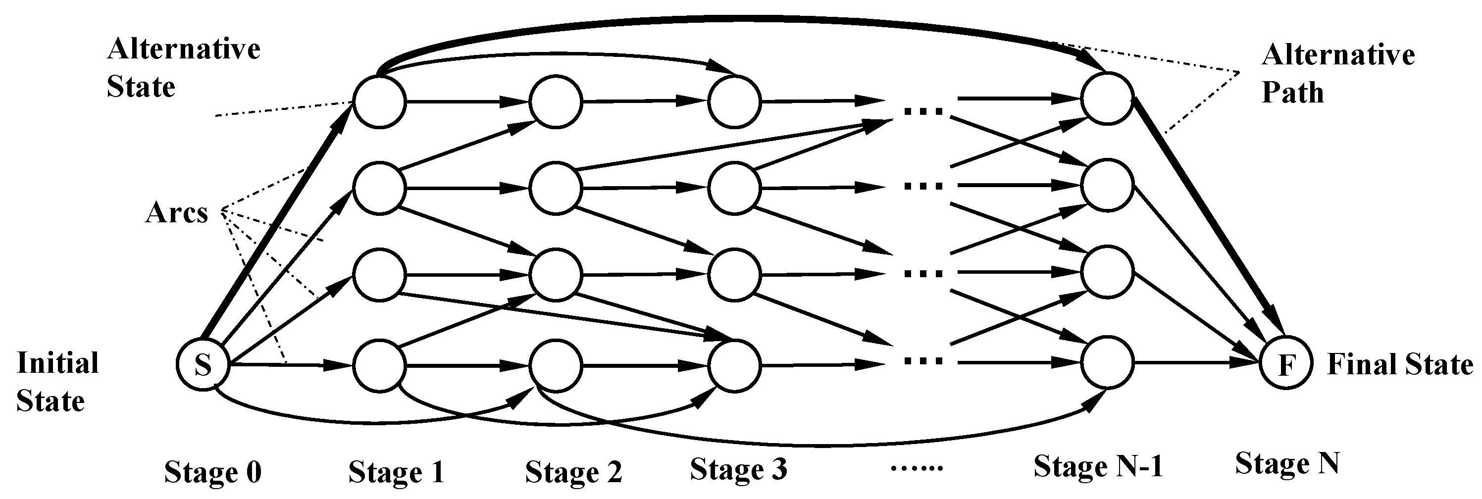
where $g_N(x_N)$ is a terminal cost incurred at the end of the process for fair evaluation of different trajectories with the same aircraft state at the final stage. Thus, generating the aircraft’s en-route trajectory can be equivalently represented by a transition graph (Figure 1), where the arcs correspond to transitions between aircraft states at successive stages, and each arc has an associated cost. Control sequences correspond to paths originating at the initial state (node S at stage 0) and terminating at end node (node F) corresponding to the final stage N. If the arc’s length is viewed as the cost, this problem is equivalent to finding the shortest path from the initial node of the graph to the end node. Here, each path is a sequence of arcs, and the length of a path is the sum of the lengths of its arcs.

With the presence of the random environment vector $y_k$, the cost is generally a random variable and cannot be meaningfully optimized. We, therefore, formulated the problem as an optimization of the expected cost:

$$E\left\{g_N(x_N)+{\displaystyle \sum _{k=0}^{N-1}{g}_k(x_k,u_k,y_k)}\right\},$$

(18)

where the expectation is with respect to the joint distribution of the random variables involved. The optimization is over the controls $u_0,u_1,\dots ,u_{N-1}$, and each control $u_k$ is selected with some knowledge of the current state vector $x_k$. Then, the class of control laws is considered that consists of a sequence function:

$$\pi =\left\{{\mu }_0,\dots ,{\mu }_{N-1}\right\},$$

(19)

where ${\mu }_k$ maps states $x_k$ into controls $u_k={\mu }_k(x_k)$ and is such that ${\mu }_k\left(x_k\right)\in {\mathbf{R}}^2$ for all $x_k\in {\mathbf{R}}^2$. Thus, for a fixed initial state $x_0$ and given functions $g_k$, the optimal cost is denoted by

$$J_{\pi \ast }(x_0)=\min E\left\{g_N(x_N)+{\displaystyle \sum _{k=0}^{N-1}{g}_k(x_k,u_k,y_k)}\right\},$$

(20)

where ${\pi }^{\ast }$ is the optimal policy that can minimize the expected cost function.

Several state transition and path constrains are also considered for en-route flight envelope protection, such as Equations (21)–(26). Bounds are placed on the control variables, state variables, and some performance parameters.

• Subject to the thrust constraint

  $$T_{\min }\le T\le T_{\max }.$$

  (21)
• Subject to the flight path angle constraint

  $${\gamma }_{\min }\le \gamma \le {\gamma }_{\max }.$$

  (22)
• Subject to the velocity constraint

  $$V_s\le v\le V_{mo};$$

  (23)

  $$-6\%\le \left(v_{k+1}-v_k\right)/v_k\le 3\%.$$

  (24)
• Subject to altitude constraints

  $$h\le H_{mo};$$

  (25)

  $$\left|h_{k+1}-h_k\right|\le 600.$$

  (26)

In the above, $T_{\min }$ is the minimum thrust, $T_{\max }$ is the maximum thrust, ${\gamma }_{\min }$ is the minimum flight path angle, ${\gamma }_{\max }$ is the maximum flight path angle, $V_s$ is stall speed, $V_{mo}$ is the maximum speed, $v_k$ is the cruise speed in stage k, $v_{k+1}$ is the cruise speed in stage k+1, $H_{mo}$ is the maximum altitude, $h_k$ is the cruise speed in stage k, and $h_{k+1}$ is the cruise speed in stage k+1.

In addition, during the transition states between stages, all aircrafts are supposed to change altitudes first, followed by speed adjustments for calculating the arcs cost in the same procedure. There is no arc between two states at the same stage in the transition graph because airborne holding will not be considered at the time of making the flight plan. Also, subject to the performance of the aircraft, some states between different stages may also have no arc since the aircraft cannot finish changing states within the distance between two stages.

In conclusion, trajectory optimization for the cruise flight is transited to a deterministic finite-state problem, which is equivalent to a special type of shortest path problem with specified state transition times, and the dynamic programming algorithm is adopted in the paper to solve this practical problem. In particular, in a deterministic problem with a continuous space character, optimal control sequences may be found by deterministic variational techniques such as steepest descent, conjugate gradient, etc. These algorithms, when applicable, are usually more efficient than the dynamical programming algorithm. However, the dynamical programming algorithm has a wider scope of applicability since it can handle difficult constraint sets such as integer or discrete sets like our model. Furthermore, it leads to a globally optimal solution, as opposed to variational techniques and popular heuristic algorithms, for which this cannot be guaranteed in general.

The program was written in Python, and Dijkstra’s algorithm was used for problem solving. The time complexity of dynamic programming was in O (E·logV), where E is the number of edges for en-route trajectory in each stage, and V is the number of nodes that is the product of alternative cruising speeds and flying altitudes. In general, the computational times were about 5.2 min for each replication when using an IBM250 with 6 GHz AMD A8 CPU and 4G RAM.

4. Numerical Test

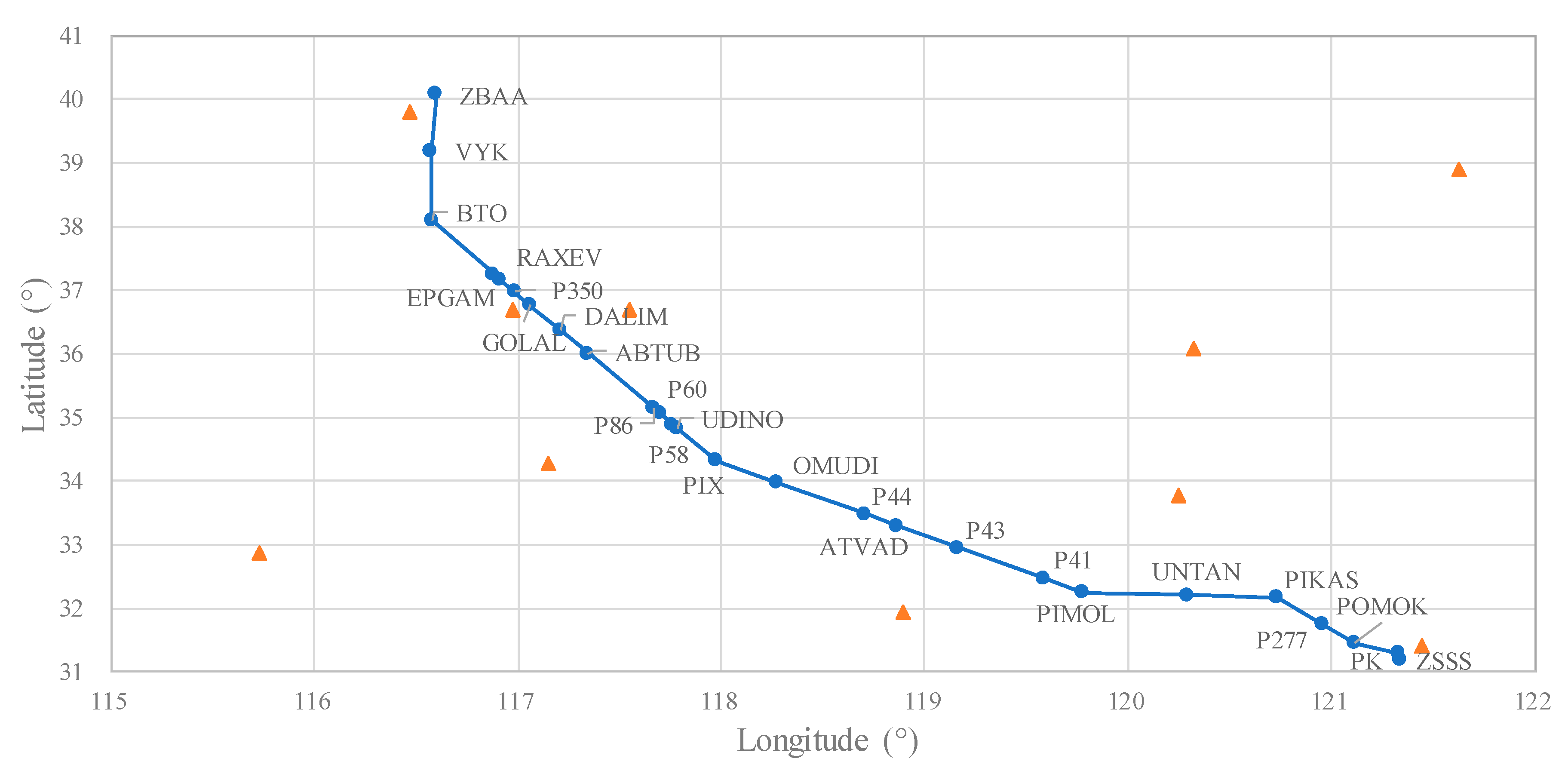
This paper selected the route ZSSS-ZBAA as a research object. ZSSS-ZBAA has 26 waypoints, and the list includes: ZSSS, PK, POMOK, P277, PIKAS, UNTAN, PIMOL, P41, P43, ATVAD, P44, OMUDI, PIX, UDINO, P58, P60, P86, ABTUB, DALIM, GOLAL, P350, RAXEV, EPGAM, BTO, VYK, and ZBAA. A sketch map is shown in Figure 2. There are 25 legs on the route.

4.1. Data Collection and Pre-Process

(1) Meteorological conditions

Meteorological conditions will affect aerodynamics, fuel flow, cruise time, and contrail generation. Because weather changes are stochastic, the randomness of meteorological data should be considered to optimize the GDOC. Therefore, it is necessary to excavate the changing law of meteorological conditions through the analysis of historical data.

a. Track wind

The track wind changes the aircraft’s ground speed, and the flight time will be different in the same ground distance, so the time cost will change.

Although the track wind is variable, there are some distribution laws. This study collected historical sounding data of sounding stations surrounding the route ZSSS-ZBAA (the triangles in Figure 2 are sounding stations). The leg PIX-UDINO was chosen to analyze the law, the meteorological parameters of this leg were calculated by using the inverse distance squared (IDS) method, and protracted histograms of track wind distributions of different altitudes (9800, 10,400, and 11,000 m) are shown in Figure 3.

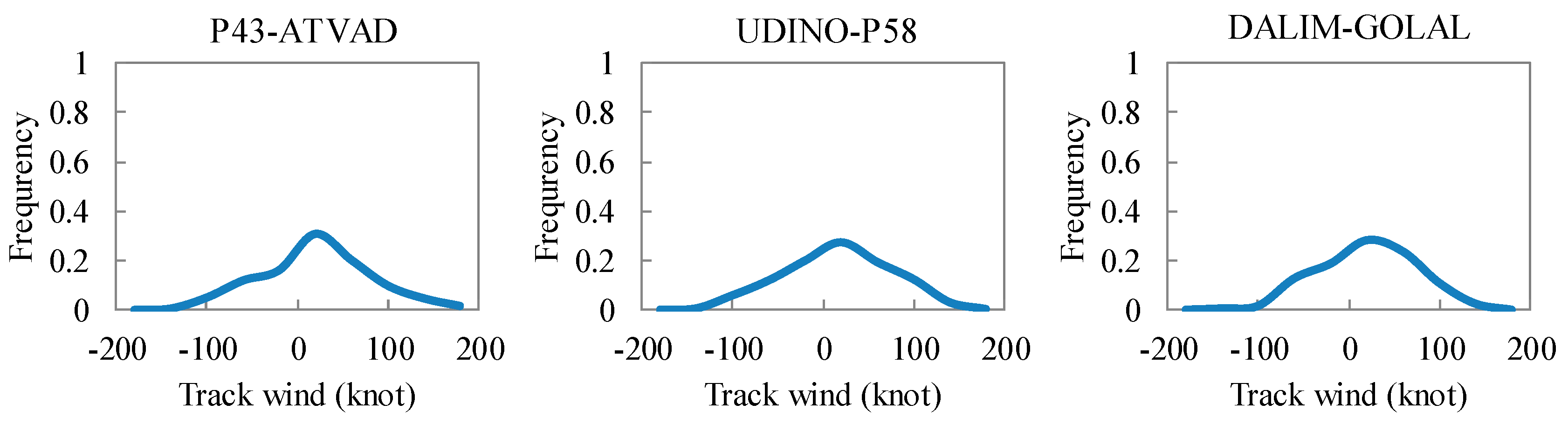
As seen in Figure 3, track wind distributions satisfy certain probability distributions, and similar results of other legs (P43-ATVAD, UDINO-P58, and DALIM-GOLAL) are drawn in Figure 4. Therefore, the mathematical expectation of track wind is regarded as the average track wind.

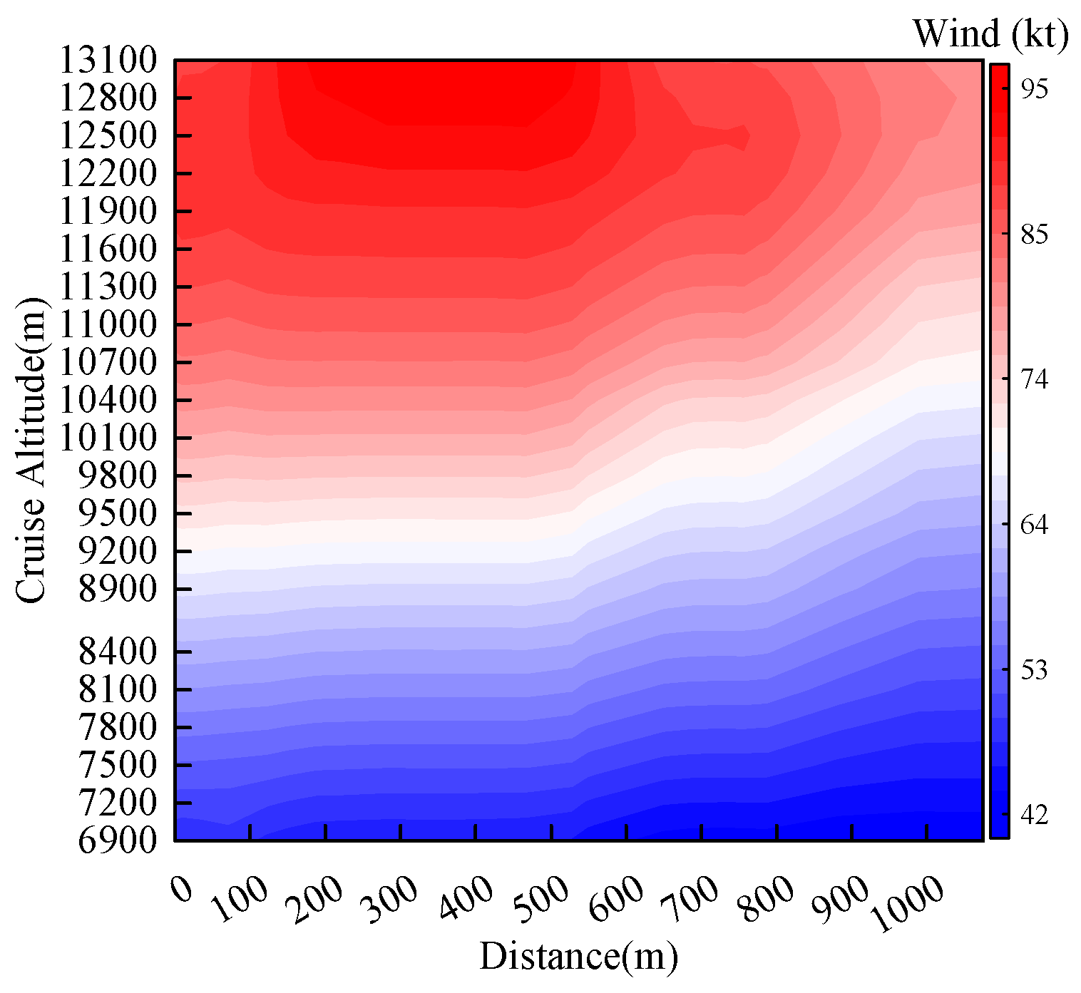
The average track winds of the route at different altitudes were calculated, and the results are shown in Figure 5. The average track wind is larger at cruise altitude.

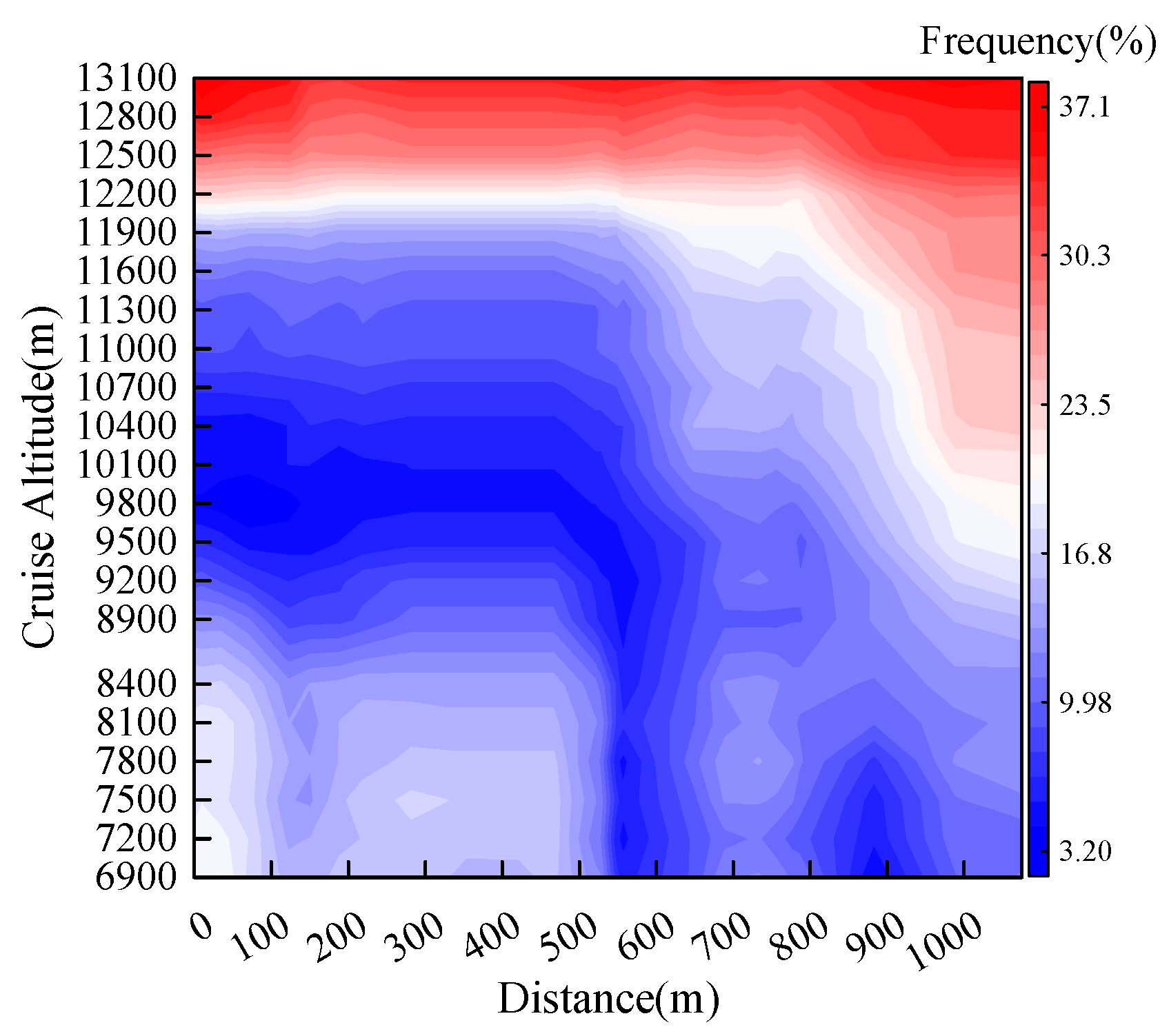
b. Contrail

Generation of contrails is determined by meteorological conditions, the probability of generation can be calculated using meteorological parameters, the results are protracted in Figure 6, and the generation probability above 12,200 m is larger than lower altitude.

(2) Performance data

This numerical test took B738 (B737-800) as an example. The flight performance parameters of B738 can be obtained from BADA, as shown in

Table 2. Performance parameters of B738.

No.	Parameter	Value	No.	Parameter	Value	No.	Parameter	Value
1	S	124.65 m2	6	CD0	0.025452	11	CTC1	146590
2	mref	65.3 ton	7	CD2	0.035815	12	CTC2	53872
3	Vs	149 knot	8	Cf1	0.70057	13	CTC3	3.0453E-11
4	Vmo	0.82	9	Cf2	1068.1	14	CTC4	9.6177
5	Hmo	12,496 m	10	Cfcr	0.93	15	CTC5	0.0085132

. Among them, m_ref is the reference aircraft mass, and No 6–15 are aerodynamic parameters to calculate the lift (L), drag (D), and thrust (T) [31].

4.2. Results

In order to better analyze the optimal results, this study set up eight scenarios (

Table 3. The information of eight scenarios.

Scenario	1	2	3	4	5	6	7	8
Objective (minimize)	Green direct operating cost (GDOC)	GDOC	GDOC	GDOC	DOC	DOC	DOC	DOC
Cruise steps (j)	1	2	3	unlimited	1	2	3	unlimited

) to carry out the case study. The cruise steps (j) mean that the aircraft changed the cruise altitude and/or speed j times along the route.

The basic parameters are set: CI = 30 kg/min, time horizon of the contrail is 25 years, the available cruise range of cruise speed is Mach 0.75–0.82, and the available cruise range of cruise altitude is 7200–12,200 m. By using dynamic programming mentioned in Section 3, the optimal results of different scenarios can be calculated and are shown in

Table 4. Optimal results (each cost, USD$) of different scenarios.

Scenario	Fuel	Time	Emissions	Contrail	DOC	GDOC
1	951.91	1260.34	175.29	1463.15	2212.25	3850.69
2	955.49	1215.86	178.53	1345.17	2171.34	3695.04
3	972.26	1219.03	182.71	1296.65	2191.29	3670.65
4	946.91	1230.44	172.24	1312.56	2177.36	3662.16
5	770.10	1314.93	121.45	3528.94	2085.03	5735.41
6	774.85	1281.69	120.41	2692.33	2056.54	4869.28
7	755.30	1257.14	113.71	3407.09	2012.44	5533.23
8	764.83	1246.18	113.57	3293.74	2011.01	5418.32

.

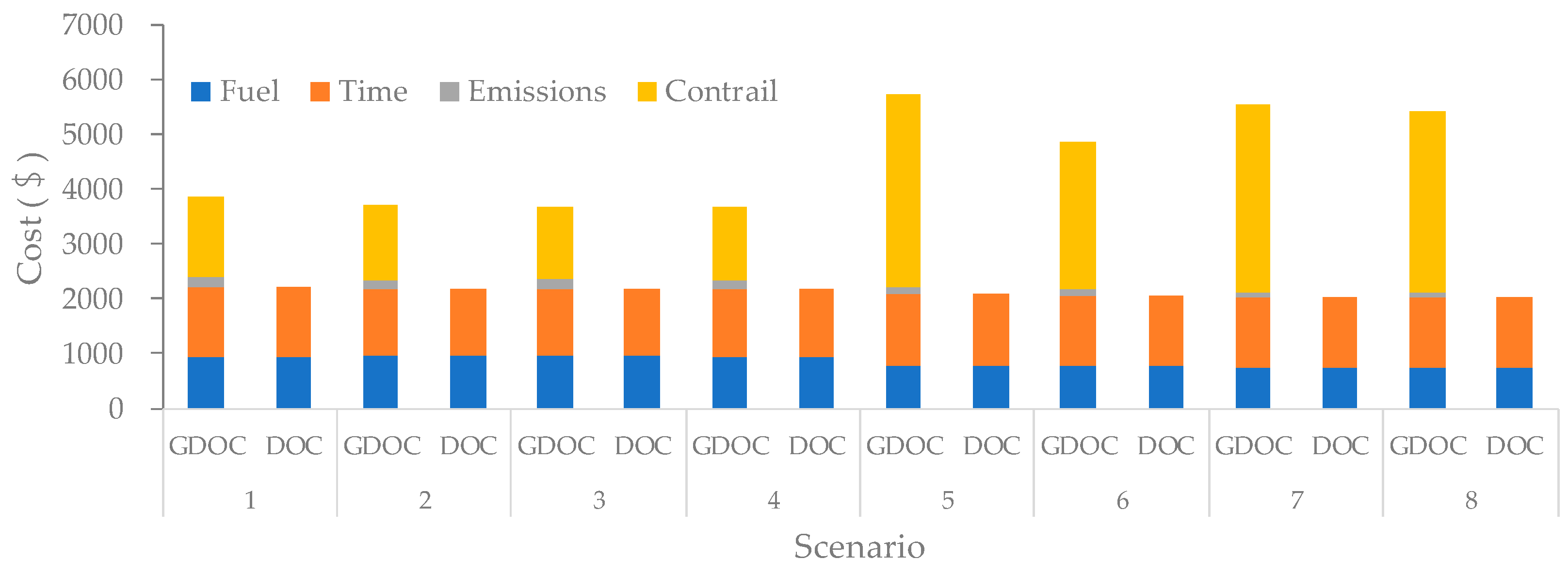
As seen in Table 4, the GDOC in scenarios 5–8 were obviously larger than in scenarios 1–4 because the objective of scenarios 5–8 was DOC and did not consider the emissions and contrail costs. However, the DOC in scenarios 5–8 were smaller than in scenarios 1–4. Compared with scenarios 1–4, scenarios 5–8 had higher contrail and time costs, and they had lower fuel and emission costs.

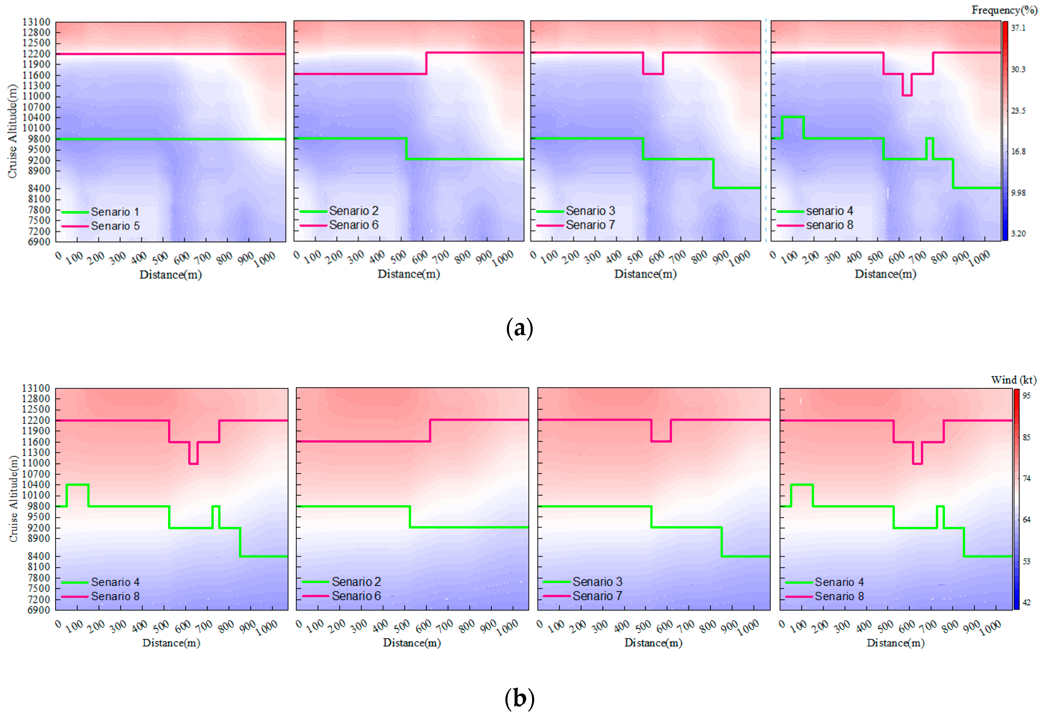
Scenarios 5–8 just aimed to minimize DOC in order to reduce the sum of the fuel and time costs. The aircraft preferred to choose the higher altitude because the aircraft’s fuel flow decreased with increasing cruise altitude. The optimal choices of cruise altitude are shown in Figure 7. The cruise altitude was 12,200 m in scenario 5.

When considering emission and contrail costs, the cruise altitudes of scenarios 1–4 were lower than scenarios 5–8. As seen in Figure 7a, the optimal cruise altitude was located at an altitude with a lower contrail frequency (9800 m and below), but the fuel costs of scenarios 5–8 increased about 20% because of a lower cruise altitude. The emission cost was relatively smaller compared with the other three costs, and it was proportional to the fuel cost. The change law of the emission cost was similar to the fuel cost.

Additionally, the wind will change the ground speed and affect the time cost, but the ground speed is the vector sum of wind speed and true airspeed, which is closely related to the atmospheric conditions of the flight level. Even if the tailwind at a certain cruise altitude is larger, the ground speed may be smaller because of the smaller true airspeed, and it will increase the time cost. Thus, the time cost of scenarios 1–4 are less than scenarios 5–8, although the tailwind optimal cruise altitude of scenarios 1–4 were smaller than scenarios 5–8, as seen in Figure 7b.

In each scenario, the flight is faster to reduce the time cost, so the cruise speed is the biggest in the optional range. Except scenarios 1 and 5, the aircraft changes its cruise altitude and/or speed. Changes are especially frequent for scenarios 4 and 8 because the cruise steps of this scenario were not limited, and the aircraft could cruise freely. The reason for this change is that the temperature, pressure, density, track wind, and contrail formation at each cruise altitude along the route were different. These differences of parameters may change the fuel flow, flight time, and emission index of aircrafts, leading to variations in fuel, time, emission, and contrail costs, so aircrafts needed change the cruise altitude in order to optimize the GDOC. It can be seen from Figure 8 that cruise speed held a line at Mach 0.82, and the cruise steps (j) were mainly embodied in the cruise altitude. These results show that the cruise altitude has a greater effect on GDOC than the cruise speed.

GDOC decreased from scenario 1 to scenario 4. These optimal results show that GDOC can be reduced by dividing the route into several steps. In other words, GDOC can be reduced by step cruise. Besides, GDOC decreased with the increase of cruise steps (j). The cruise in Scenario 2 was in two steps (j = 2). The GDOC decreased about 4.0% compared to the result in scenario 1 (j = 1), and when cruising in three steps (j = 3), the result decreased about 4.7% compared to scenario 1. If the times of the cruise steps are not constrained, the aircraft can choose the cruise altitude and speed freely according to GDOC; the optimal result is shown in scenario 4, were GDOC decreased by about 4.9%. In other words, the reduction of GDOC decreased with j. The result of scenario 4 is the global optimal solution, but high frequencies of altitude and speed variations will cause a heavier workload for pilots. The optimization effects of scenario 2 and scenario 3 were very close to scenario 4, as seen in Figure 9, so in actual flight, the aircraft can choose cruise steps 2 or 3 to lighten the pilot’s workload.

The results above are under the given conditions of aircraft type, time horizon, and cost index. When the given conditions change, the optimal results will change accordingly. The discussion is as follows:

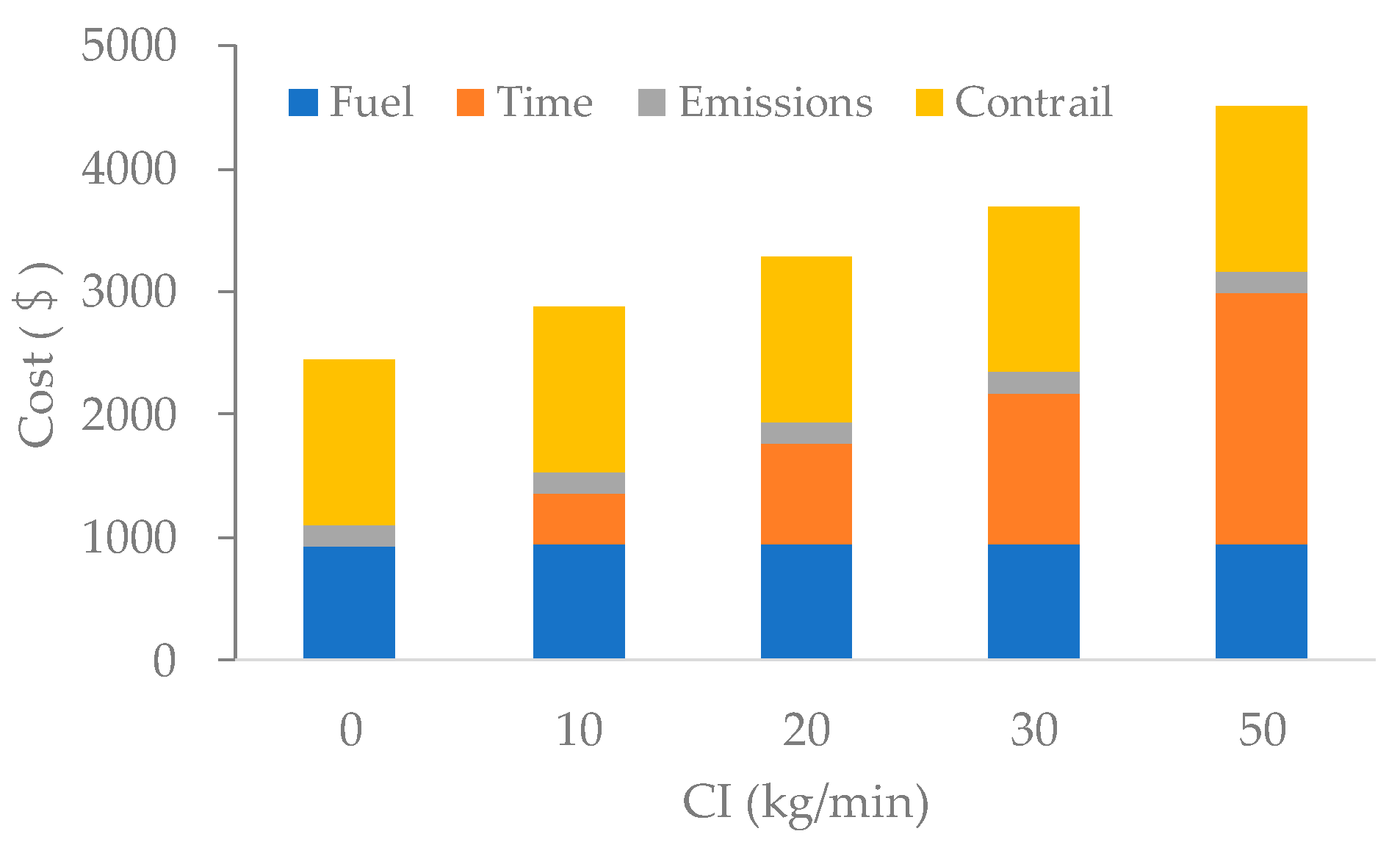
The time cost varied based on cost index CI. Using the example of B738 above where CI = 30, when the value of CI changes, the optimal results will change, as shown in

Table 5. The optimal results of different cost index (CI) values in each scenario ($).

CI (kg/min)	Fuel	Time	Emissions	Contrail	GDOC
0	939.85	0.00	165.41	1346.47	2451.73
10	944.00	418.93	171.14	1346.58	2880.65
20	955.49	810.57	178.53	1345.17	3289.76
30	955.49	1215.86	178.53	1345.17	3695.04
50	955.49	2026.43	178.53	1345.17	4505.61

.

A higher CI means a higher time cost. The time cost and GDOC increased from CI = 0 to CI = 50, as seen in Figure 10. Changes in fuel, emission, and contrail costs are not obvious, especially when CI > 20, as these costs remain unchanged.

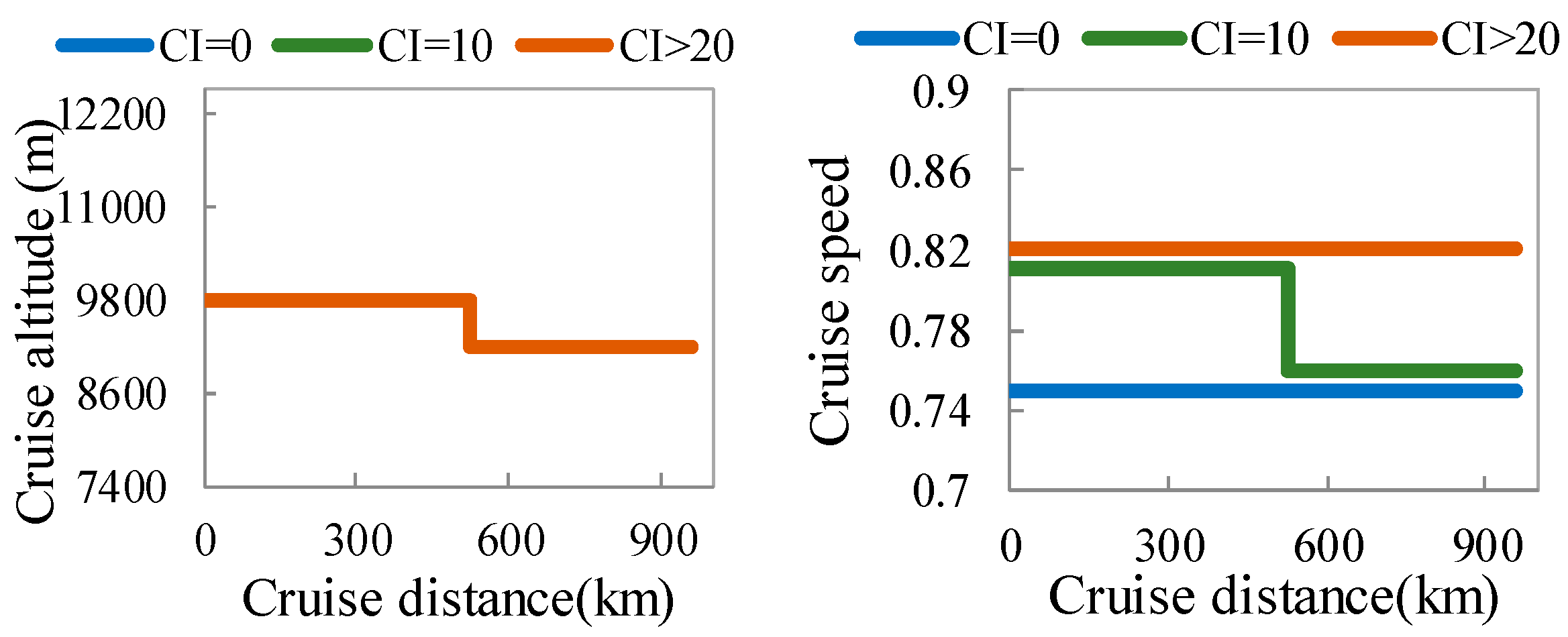
The cruise altitude and speed profiles of different CI values are shown in Figure 11. A bigger CI requires the aircraft to fly faster, so the cruise speed increases as CI increases.

The optimal results of different aircraft types are shown in

Table 6. The optimal results of China Eastern Airlines.

Type	CI (kg/min)	Volume	GDOC (Scenario 6) ($)		GDOC (Scenario 2) ($)
			Single	Annual (106)	Single	Annual (106)
B738	30	644	4869.28	3.14	3695.04	2.38
A320	20	10	4386.79	0.04	3393.20	0.03
A321	25	1182	4208.29	4.97	3726.87	4.41
A332	40	82	6918.13	0.57	5227.95	0.43
A333	40	4248	6683.31	28.39	5212.70	22.14
B767	40	251	5572.28	1.40	5315.35	1.33
B777	90	652	7708.50	5.03	7574.59	4.94
Total	-	7069	-	43.54	-	35.66

. The cost index (CI) of each aircraft type are derived from the airline’s historical data. Take China Eastern Airlines (CES) as an example; there were 7069 flights on route ZSSS-ZBAA in 2017, and the annual cost of each aircraft type are shown in Table 6.

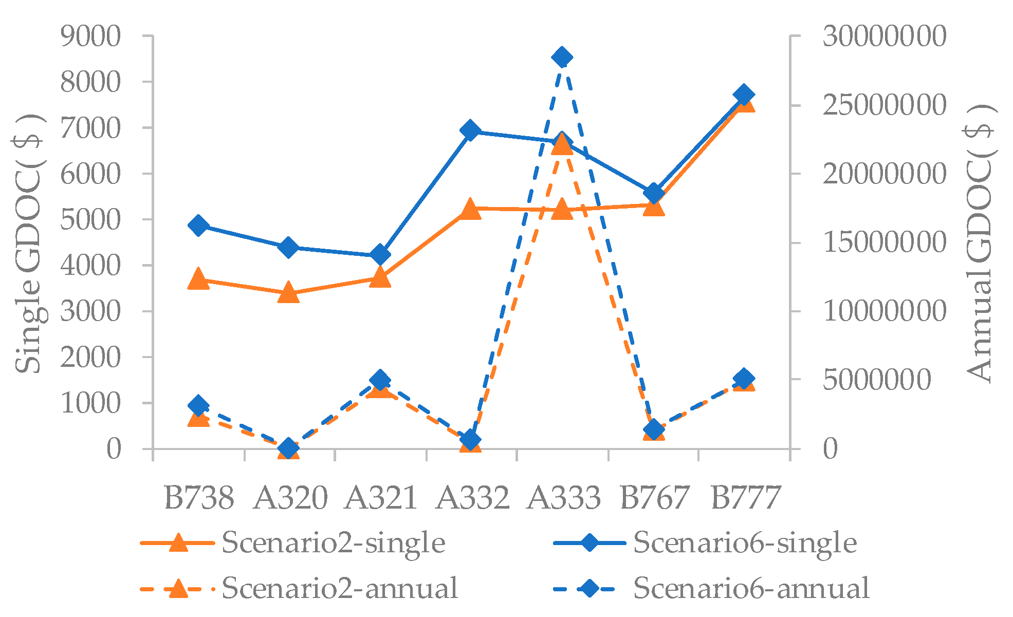
The annual GDOC distribution of each aircraft type were different from the individual, because the volume of each aircraft type was different, as seen in Figure 12. The single GDOC of A333 was not the largest, but its annual GDOC was more than the other types because of its volume (4248 sorties).

When comparing the annual GDOC of Scenario 2 and Scenario 6, China Eastern Airlines could have saved GDOC 7.87 million US dollars in 2017 if the environmental cost was considered.

5. Conclusions

In order to analyze the sustainable development and operational cost of civil aviation reasonably, this paper constructs a GDOC model by adding the environmental cost into the airline’s DOC, and it optimizes the GDOC by choosing the cruise altitude and speed. The main research contributions are as follows:

(1)

This paper modeled the pollutant gas and greenhouse gas (CO₂) cost with the flight performance model and engine characteristics, and then it deduced the contrail cost model by comparing the greenhouse effect with CO₂. The GDOC was finally constructed with four parts—fuel, time, emissions, and contrail costs—and the calculation methods were given.

(2)

An optimal control measure was proposed to minimize GDOC that considered uncertain factors and constraint conditions (including cruise step, cruise altitude, cruise speed, etc.) using dynamic programming to search the optimal results.

(3)

The numerical test built eight scenarios and used B738 as an example. The rationality of the GDOC results were verified by comparing the results of DOC and GDOC scenarios. The optimal results of GDOC showed that the optimal choice of cruise altitude and speed could effectively reduce the environmental impact and environmental costs, while increases in fuel and time costs were small.

(4)

This paper analyzed the influencing factors in achieving optimal results. If the aircraft cruise had more steps, the GDOC was less. The cruise altitude had a greater impact on the result than cruise speed, and a lower altitude was preferred to reduce GDOC. The choice of the cruise speed will change by the increase of CI; different aircraft types have similar rules for the optimal results.

This paper studies the optimal flight performance selection problem of a flight plan. In real-time flights, in addition to the aircraft’s own performance, it is also necessary to consider flight conflicts, airspace limitation, real-time meteorological conditions, etc. Future work can be carried out by analyzing the factors that influence real-time flight performance as well as combining these influencing factors and the GDOC model to find global optimal solutions.