The Green Infrastructure Assessment System (GIAS) and Its Applications for Urban Development and Management

Abstract

Adverse changes of the landscape resulting from diverse human activities have consequently caused quality decline and functional degradation of the natural landscape, endangering the natural habitats of various species. Meanwhile, technical advancements in the area of spatial analysis including GIS and remote sensing enable many kinds of easy-to-quantify landscape indices. Although some systems were developed to support assess landscape indices, developing systems for practical decision-making in spatial planning was insufficient. In this study, the GIS-based Green Infrastructure Assessment System (GIAS) was developed for integrated assessment of diverse landscape ecological values to use in spatial planning and management based upon indices sets that are mainly represented as structure, function, and dynamics of the landscape. In order to verify the effectiveness of the system, two case studies involving the city of Namyangju, northeast of Seoul, were conducted by applying GIAS to the (1) macro scale and (2) micro scale. The study results demonstrate the capability of GIAS as a planning support tool to perform concrete assessment of landscape ecological values and performance both on the macro and micro scale, and its applicability to diverse stages in spatial planning. By utilizing GIAS, frequent human-induced impacts resulting from development projects can be examined in advance, and proactive alternatives can be prepared. In addition, effective decision-making for scientific and systematic planning and management of green infrastructure can be achieved.

1. Introduction

Human-induced activities have become the primary cause of quality decline and functional degradation of the natural landscape. In urban areas, the function of the landscape is the result of the interrelationship between physical structures based on natural processes, and human-induced activities [1,2,3]. Moreover, the dynamics of landscape patches change a landscape’s naturalness and function, and can cause changes in the distribution and appearance frequency of the inhabitants [4]. As a result, there is increasing awareness of the importance of landscape ecological planning, landscape restoration, and landscape damage prevention, which are now becoming central considerations in the spatial planning process [4]. To address the spatial dimension of sustainable planning, Leitão and Ahern [5] suggest that the landscape ecology concept and applied metrics can be used to provide a theoretical basis for landscape and urban planning. There are a number of empirical studies on landscape ecological assessments of land use changes [6,7,8,9] and on the assessment of urban landscape value for conservation [10,11,12] using these concepts and metrics. Furthermore, landscape ecology indices have been employed to establish urban ecological networks [13,14,15]

Meanwhile, green infrastructure has been regarded as a major spatial planning element to not only reduce the loss of ecosystem services concerned with urbanization but also to enhance the stability of the urban ecosystem. A green infrastructure is defined as an interconnected network of green spaces that is designed to conserve natural ecosystem values and functions. It provides related benefits to the human population [16]. There is an emphasis on the importance of quantitative assessment of ecological values and mapping of assessment results [17]. In addition, such an ecological network should be built based on connectivity analysis to meet the green infrastructure concept [17,18]. As a result, the importance of scientific assessment of landscape connectivity is emphasized. In this regard, based on planning methods of the traditional ecological network, various methodical studies on networking urban green infrastructure (e.g., Liquete et al. [17]; Zhang et al. [18]; Lee, Chon, and Ahn [19]) has been conducted.

In addition, in order to manage green infrastructure more effectively, it is crucial to monitor landscape changes due to intensive landscape changes by urban development and road construction [20,21]. Therefore, analytical approaches and research applying ecological indicators to monitoring landscape changes has been gradually increasing [21,22,23]. In particular, landscape indices have also been widely applied as a basic indicator to investigate landscape changes. The variation of landscape indices has been compared to driving forces that cause landscape changes in time series, in order to delineate conservation areas [24,25] or determine the effects of driving forces [26,27,28]. In addition, landscape capacity has also been analyzed based on landscape change analysis [29]. Recently, such research on landscape monitoring studies have been applied to decision support systems for spatial planning [20]. For effective analysis and decision-making, visualization of landscape changes through mapping is also emphasized [29].

Meanwhile, technical advancements in the area of spatial analysis including GIS and remote sensing can enhance landscape ecology theories and be applied to analyze the landscape. Some examples of such systems include FRAGSTATSs, Patch Analyst, V-Late (Vector-based Landscape Analysis), and SPAN (SPatial ANalysis program), which are used for easily quantify many kinds of landscape indices, such as area, shape, edge, and proximity. There is also LCM (Land Change Modeler) which simulates land cover changes and analyzes landscape ecology indices in time series. However, these systems have mainly focused on analyzing landscape patterns and processes rather than on practical decision-making in spatial planning. There were some initial attempts to develop a system to apply to practical decision-making in spatial planning employing landscape indices. Reynold, and Hessburg [10] developed EMDS (Ecosystem Management Decisions Support) system to determine primary conservation areas based on landscape structural assessment. In addition, Lee and Oh [30] developed LEMS (Landscape Ecological Management System) to compare landscape indices of green infrastructures on the micro scale. However, EMDS has a drawback as a landscape change monitoring tool, because it mainly focuses on selecting conservation forests on the macro scale with a single time point. In the case of LEMS, it has also been insufficient as a tool to support the green infrastructure planning process, because it mainly focused on quantitative comparison of proposed alternatives. In addition, it is difficult to identify exact locations of landscape change because it applies only Global Moran’s I to assess landscape distribution.

Despite the numerous attempts to apply landscape ecology theories to spatial planning and management, practical applications are still challenging [28,31,32,33]. This is because most studies have mainly focused on landscape spatial patterns and ecological processes on the macro scale alone [3,34], when micro scale analysis is also needed for actual implementation of spatial plans. Another reason lies in the fact that landscape ecology theory is not effectively applied in the complex decision-making process for spatial planning which is composed of problem seeking, alternative establishment, scenario analysis, and evaluation and monitoring [34]. Naveh [35] suggests the development of a systematic framework to resolve actual problems of spaces through a proper theory that involves a methodology and multidisciplinary approach. His view stems from the fact that there is an absence of an assessment framework to integrate the numerous landscape ecological indices. Therefore, concrete and sophisticated methods and tools are needed to sufficiently satisfy demands within spatial planning.

Still, degradation can be reduced while ecological value can be maintained through scientific investigation that involves identifying impaired and fragmented green infrastructure caused by human activities [31,36]. Moreover, GIS-based scientific support tools can be employed to foster effective decision-making in the spatial planning and management of green infrastructure in urban areas [21]. In this regard, this study focuses on the establishment of a decision support tool for the spatial planning process based upon landscape ecology theories. For this study, a landscape ecological assessment framework was created and consequently, the GIS-based Green Infrastructure Assessment System (GIAS) was developed for integrated assessment of diverse landscape ecological values to use in spatial planning and management. To verify the effectiveness of the system, two case studies were conducted for the application of GIAS to the 1) macro scale (city scale) and 2) micro scale (urban development scale in the city). The research questions in this study are as follows:

(1)

On the macro scale, can the times series changes of the landscape patches be detected quantitatively by the GIAS? In addition, can the spatial location where the structure and function changes of the landscape suddenly occur, be investigated?

(2)

On the micro scale, can the locations where additional corridors to enhance connectivity should be introduced in urban development project area, be identified by GIAS? In addition, can the structural and functional variations due to such small landscape changes, be detected?

(3)

As a tool for evaluating green infrastructure alternatives, is the integrated assessment of GIAS useful for decision-making? Furthermore, can changes of landscape indices be identified clearly by integrated assessment?

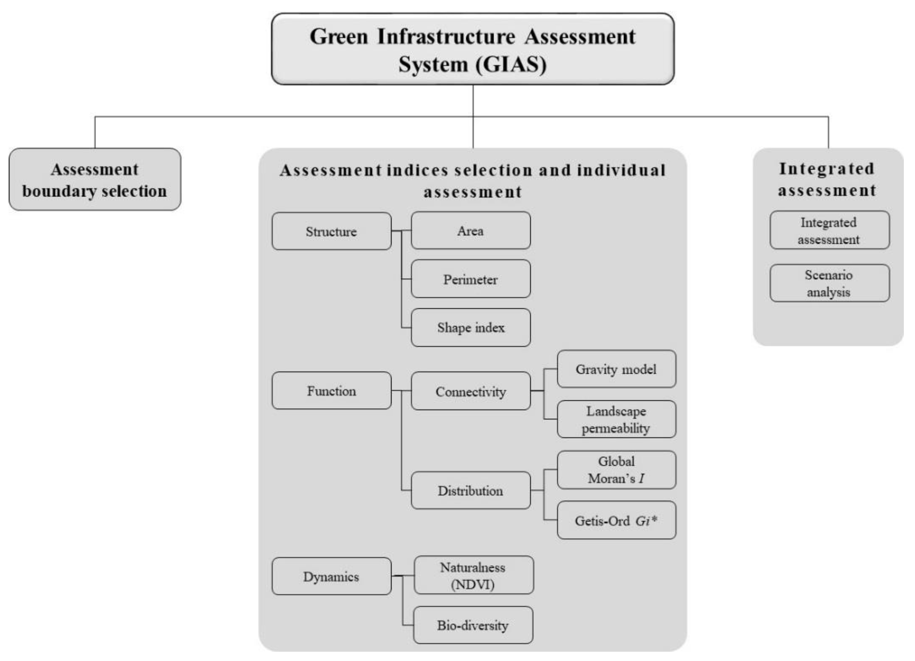
2. Material and Methods

2.1. Assessment Indices for This Study

Considering the landscape ecological importance for establishing green infrastructure, a framework consisting of diverse assessment indices was considered for this study. The first assessment index for this study is structure. Patch area and shape are primary structural indices used to explain landscape characteristics and have been widely and frequently applied to analyses on landscape structure [10,37,38]. In fact, because urban development affects the area and shape of existing landscape patches, area and shape are important aspects in urban development. Additionally, because patch area has a direct impact on inhabitants’ stability and bio-diversity, the effects of urban development can also be directly evaluated by patch area analysis [4,13,39]. From a bio-geographical perspective, patch shape is also important in analyzing the stability of species distribution, extension and reduction, and interaction with neighborhood matrices [1,37,39].

The second assessment index is function, since connectivity and distribution have been widely used as landscape functional indices. Connectivity refers to the connection probability of landscape patches and has been extensively used to assess landscape conservation value and network probability [13,34,40]. As a measurable landscape characteristic to support spatial planning, connectivity has also been applied in planning for green corridors and ecological networks [13,15,19,41]. On the other hand, distribution refers to spatial statistics between landscape patches, and has been applied to identify distribution patterns of landscape patches. Various spatial statistics methods used to quantify aspects of landscape patterns are typically used to detect the spatial auto-correlation for landscape elements [4]. Thus, distribution can be used as basic data in the restoration planning of green spaces [39].

The third assessment index is dynamics. In landscape ecology, dynamics refers to changes of landscape characteristics in time series analysis. From a dynamics perspective, Forman and Godron [1] suggest that landscape stability could be assessed by monitoring persistence, resistance, and recovery or resilience of a landscape. Thus, in the spatial planning process, dynamics is important in dealing with the monitoring and managing of ecosystems after development [42,43]. Considering the importance of sustaining inhabitants and that conserving natural resources increases in spatial planning, naturalness, and bio-diversity have been central to assessing dynamics. With the aim of achieving applicability and usefulness in spatial planning implications of the landscape assessment indices for this study were selected as

Table 1. Implications of assessment indices for this study.

Indices		Selection Basis
		Landscape Ecology Perspectives	Spatial Planning Perspectives	References
Structure	Area (Landscape patch area)	Index for the quantity of the natural environment, and widely applied to assess conservation value	Urban development causes changes of the area and shape of landscape patches, and landscape patterns	[4,10,13,30,37,39]
	Shape (Landscape patch shape)	Index for species distribution, stability and migration probability based on the edge effect		[1,30,37,39]
Function	Connectivity (Connecting probability between landscape patches)	Index for the quality of the natural environment; the probability that inhabitants’ networking can be analyzed	Index for supporting green corridors and ecological network planning	[13,15,30,38,40]
	Distribution (Distribution of landscape patches)	Index for the arrangement of landscape patches; distribution patterns of landscape patches can be analyzed	Urban development causes changes to existing landscape patterns by introducing new landscape patches and damaging existing patches	[4,30,39]
Dynamics	Naturalness (Naturalness of landscape patches)	Index for naturalness and the soundness of landscape patches; conservation value of landscape patches can be analyzed	Index for estimating landscape dynamics due to landscape changes	[1,4,13,30]
	Bio-diversity (Frequency of different species and their diversity)	Index for the quality of the natural environment; land use change causes variations of existing inhabitant distribution and appearance		[1,4,12,30]

.

2.2. Assessment Methods

2.2.1. Landscape Structure

In order to assess landscape structure in this study, landscape patch area and shape index with the number of landscape patches were estimated. The larger patch area is considered to have a better landscape ecological value based on Conservation Biology [1,44,45]. In the case of shape index, the lower index indicates a better value [1,4] in terms of bio-diversity and landscape stability (

Table 2. Criteria for assessing landscape structure.

Indices		Measurement	Interpretation	References
Landscape patches		The total number of landscape patches	The more individual landscape patches are integrated into large patches, the more favorable they are for suitable habitats	[1,4,13,44,45]
Area	Total area	The total area of landscape patches (ha)
	Mean area	The mean area of landscape patches (ha)
Mean shape index		The ratio of area and perimeter $D_i=\frac{P_i}{2\sqrt{A_i\pi }}$ Di: shape index of landscape patch i Pi: perimeter of landscape patch i Ai: area of landscape patch i	A lower index (similar to round shape) is favorable for species’ richness, bio-diversity, and landscape stability	[1,4]

).

2.2.2. Landscape Function

The landscape function in GIAS includes connectivity and distribution. To assess connectivity, the network structure of landscape patches was analyzed using the gravity model which can measure the spatial interaction of landscape patches quantitatively [1,4]. The best routes for networking were then identified based on the gravity analysis results and accumulated friction values [5,14,15,40] were calculated by least-cost path analysis.

On the other hand, landscape fragmentation was assessed by analyzing the distribution of landscape patches [4,13,38] and the correlation of landscape patterns using spatial auto-correlation. The separation distance of the landscape patches was estimated and the spatial auto-correlation of landscape patches of the entire area was analyzed adopting Global Moran’s I [9,39]. Meanwhile, hot spots (or cold spot) which indicated a strong probability of landscape patch changes in patch area or shape index were identified employing Getis-Ord G_i* which could measure concentrations of high or low values for the entire area [39,46]. If the Z-score of Getis-Ord G_i* was higher than 1.96, the areas were classified as hotspots whereas areas that scored lower than −1.96 were classified as cold spots (Z-score < −1.96) (

Table 3. Criteria for assessing landscape function.

Indices		Measurement	Interpretation	References
Connectivity	Gravity index	$G_{ij}=k\frac{\left(P_i\times P_j\right)}{D_{ij}^2}$ Gij: interaction between patch i and patch j Pi: amount of objects in patch i Pj: amount of objects in patch j Dij: distance between the patch i and patch j k: constant value	Higher number of networks and higher indices are favorable	[4,38]
	Least-cost path	Ni + 1 = Ni + (ri + ri + 1)/2 i: Origin cell, i + 1 = Target cell ri = Friction value in cell i Ni = Accumulated cost in cell i	Landscape permeability: how freely animals can move through a landscape; analyzing the best route for target species migration; lower accumulated fraction value is favorable	[5,14,15,40]
Distribution	Separation distance	The average separation distance of landscape patches (m)	Shorter distance is favorable	[4,13,38]
	Moran’s I	$I=\frac{n}{S_0}\frac{{{\displaystyle \sum }}_{\mathrm{i}=1}^{\mathrm{n}}{{\displaystyle \sum }}_{\mathrm{j}=1}^{\mathrm{n}}{\omega }_{ij}{z}_i{z}_j}{{{\displaystyle \sum }}_{\mathrm{i}=1}^{\mathrm{n}}{z}_i^2}$ n: the number of patches indexed by i and j wij: spatial weigh between patch i and patch j S0: aggregate of all spatial weight zi: (xi-X) deviation of an attribute for patch i If the index value is greater than 0, the set of features exhibits a clustered pattern. If the value is less than 0, the set of features exhibits a dispersed pattern.	Higher index (gathered for similar shape and area) is favorable	[9,39]
	Getis-Ord Gi*	$G_i^{*}=\frac{{{\displaystyle \sum }}_{\mathrm{j}=1}^{\mathrm{n}}{\omega }_{i,j}{x}_j-\overline{X }{{\displaystyle \sum }}_{\mathrm{j}=1}^{\mathrm{n}}{\omega }_{ij}}{S\sqrt{\frac{[\mathrm{n}{{\displaystyle \sum }}_{\mathrm{j}=1}^{\mathrm{n}}{\omega }_{i,j}^2-({{\displaystyle \sum }}_{\mathrm{j}=1}^{\mathrm{n}}{\omega }_{i,j})]}{n-1}}}$ xj: attribute value for patch j wij: spatial weight between patch i and patch j $\overline{X}=\frac{{{\displaystyle \sum }}_{\mathrm{j}=1}^{\mathrm{n}}{x}_j}{n}$$,S=\sqrt{\frac{{{\displaystyle \sum }}_{\mathrm{j}=1}^{\mathrm{n}}{x}_j^2}{n}-{\left(\overline{X}\right)}^2}$	Hot spot or cold spot areas have a strong probability of landscape patch damage	[39,46]

).

2.2.3. Landscape Dynamics

For this study, landscape dynamics were assessed in terms of naturalness and bio-diversity. In order to assess forest dynamics, the rates and patterns of landscape changes were investigated mainly with remote sensing techniques using satellite imagery. The assessment results can provide useful information to guide future management directions. To assess landscape naturalness, the Normalized Difference Vegetation Index (NDVI) which is the most common type of analysis used for green space was adopted. To estimate the variation of landscape naturalness, NDVIs were calculated from remote sensing data of two or more time points, and variations of NDVI were compared. Meanwhile, bio-diversity could be assessed by species’ characteristics and the variety of landscape patches [12,36,47,48]. Areas where diverse species have been identified are considered as possessing relatively high bio-diversity within a food chain [36]. Therefore, bio-diversity was assessed by estimating the number of types of species and the number of identified areas of species in the landscape patches (

Table 4. Criteria for assessing landscape dynamics.

Indices	Measurement	Interpretation
Naturalness	Normalized Difference Vegetation Index $NDVI=\left(\frac{NIR-VIS}{NIR+VIS}+1\right)\times 128$ NIR: spectral reflectance measurements acquired in the near-infrared regions VIS: spectral reflectance measurements acquired in the visible regions Range: 0–255	Higher is favorable	-
Bio-diversity	The number of types of species and the number of identified areas of inhabitants in landscape patches	Identified landscape patches which have more types of species and inhabitants in the area is favorable	[47,48]

).

2.3. Developing GIAS

This study developed the GIS-based Green Infrastructure Assessment System (GIAS) for integrated landscape ecological assessment. The major analytical function of the system consists of assessment boundary selection, assessment indices selection and individual assessment, and integrated assessment (Figure 1). Considering the assessment site scale, the assessment boundary selection function allows for the selection of the assessment area and can include patches of interest near the assessment area. The assessment indices selection and individual assessment function are used to select and assess individual landscape ecological indices (structure, function, and dynamics).

Meanwhile, a multi-level approaches are essential for in-depth analysis of the structure-function-dynamics of landscape patches. Therefore, GIAS was developed to enable analysis of patch scale and class level analysis considering the green infrastructure planning management process rather than focusing on specific levels. In the integrated assessment, the results for the individual indices are mapped out sequentially and a comprehensive table for interpreting the assessment results is presented. The detailed procedure is as follows:

The structures (area, circumference, and shape) of each individual green infrastructure are analyzed at the patch level. The results are mapped in a polygon vector format. Next, the function assessment is performed based on the structure assessment results at the class level. In order to analyze connectivity and distribution, the separation distance between the green infrastructures is input as an analysis parameter for gravity model analysis and spatial autocorrelation analysis. The result of the gravity model analysis is mapped in a line vector format, and the gravity index is calculated as an attribute table on each line. Based on the gravity model results, considering landscape permeability, least-cost path analysis is performed to determine the best route to connect separated green infrastructure. The least-cost path analysis is also delineated as a line vector, and the cumulative friction values of each line are stored as on an attribute table. On the other hand, the distribution pattern of the green infrastructure is analyzed by applying Global Moran’ I based on the area or shape index of the individual green infrastructure. Next, the local distribution of green infrastructure is assessed by Hot spot analysis (Getis Ord Gi*). The results of hot spot analyses are mapped in a polygon vector format, and the z-scores and p-values of each green infrastructure are presented as an attribute table. Finally, each result is summarized at the class level. Thus, the integrated assessment function assessed the landscape ecological characteristics comprehensively so that the user could identify the assessment results more ease. Meanwhile, the scenario analysis function was developed to compare the integrated assessment results which change according to various alternatives and conditions. An input and output data format for the assessment and integrated assessment results using GIAS is presented in Appendix A.

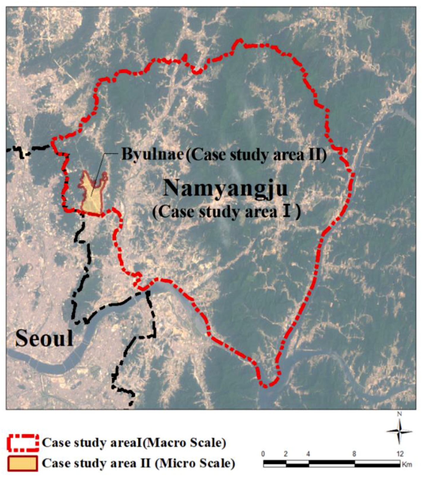
2.4. Developing GIAS Case Studies on the Macro Scale (City Scale) and Micro Scale (Urban Development Project Scale)

Landscape planning and management have tended to focus mainly on areas using the regional scale (macro scale) in Korea. Recently however, recognition of the importance of human-induced green space construction in urban development processes (micro scale) has been increasing. Therefore, more concrete and elaborate analyses of development plans are being required to verify their landscape ecological performance. In this regard, case studies for this study were conducted applying GIAS to two levels of scale: the macro scale and micro scale to verify the practicality of the system for spatial planning and management. In the first case study, changes of the landscape ecological value in the entire area of a city were assessed through time series analysis. On the macro scale, the usefulness of GIAS as a monitoring tool to manage landscape resources in the entire area was examined.

In the second case study, the usefulness of GIAS as a planning support tool to enhance landscape ecological performance of a specific urban development plan was examined for part of a city (micro scale). The landscape ecological performance of urban development in this study refers to whether a proposed development plan is suitable with regard to landscape ecological theories. Among the three ecological assessment indices (structure, function, and dynamics), the dynamic index was excluded for the micro scale case study because the proposed plan has been implemented recently and, thus, long-term landscape changes cannot be observed yet.

2.4.1. The Study Areas

The area for Case Study 1 is the entire area of Namyangju, a northeastern city adjacent to the Seoul Metropolitan Area. The total area of Namyangju is about 458.5 km², housing approximately 476,000 residents. More than half of Namyangju was designated as a conservation area due to the presence of favorable green spaces. However, development pressure has been increasing substantially in recent years. Subsequently, effective landscape management is required due to the substantial reduction of forest areas caused by various urban development and road construction projects.

For case study 2, the Byulnae new town project area in the western part of Namyangju was investigated. This area has been released from the green belt area by the government and as a result, this large new town project is currently underway. The development area is about 5 km² with about 76,000 people projected to inhabit this area. Most of the area is planned for residential use while the remaining amount or about 28.6% is planned for green spaces using landscape resources, such as existing forests and streams (Figure 2). For this reason, a growing major concern is whether or not the provision of new green space with the development plan in the former green belt will still be able to accommodate landscape ecological soundness.

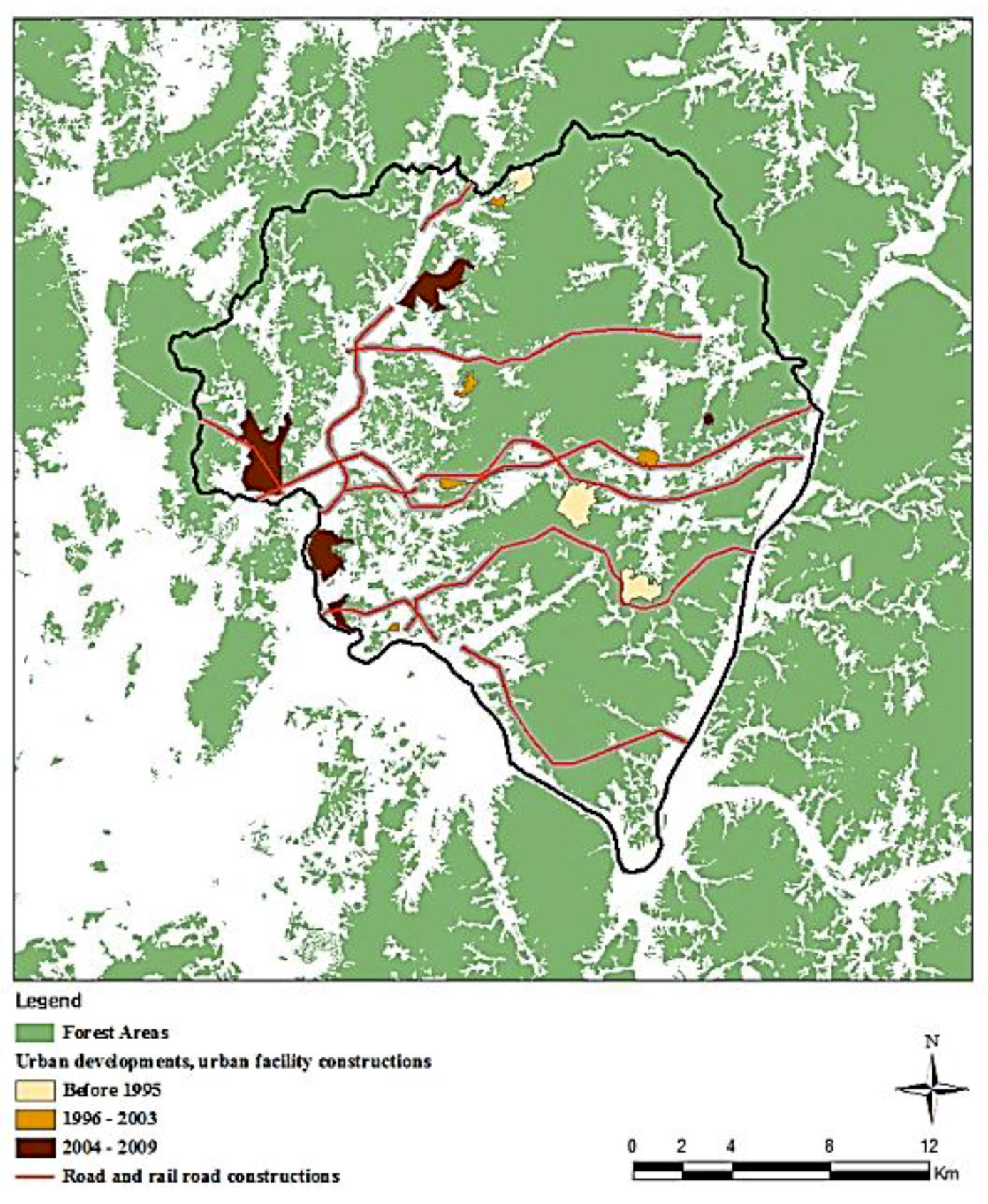
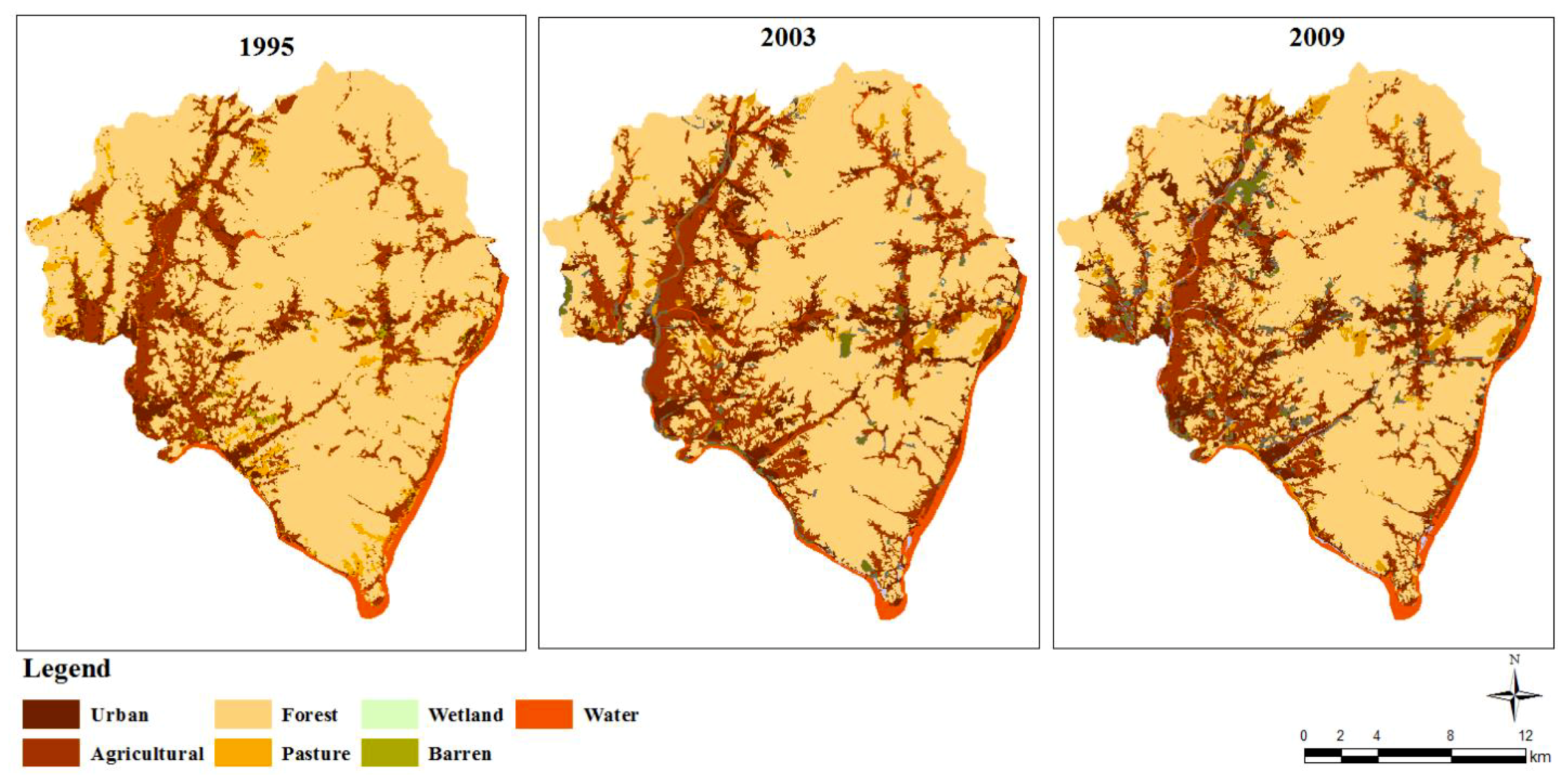
2.4.2. Case Study 1: Macro Scale Application for Landscape Management

Identifying the variations of landscape patches by driving forces could be useful in monitoring urban green infrastructures [28,49]. In Case Study 1, the major urban developments in the study area were investigated. In addition, landscape value changes in the entire area of Namyangju are assessed in terms of structure, functions (distribution and connectivity), and dynamics (naturalness) through time series analysis. The 30 × 30 m resolution land cover maps that were prepared through surveys in 1995, 2003, and 2009 by the Korean Ministry of Environment were utilized. The landscape patch data for urban forests, which are the most important green infrastructure on the macro scale, were extracted from the land cover maps for these years in order to maximize the accuracy of the assessment. Then, landscape changes were observed.

2.4.3. Case Study 2: Micro Scale Application for Landscape Ecological Performance Assessment of a New Town Project

Three stages consisting of no development, original development plan, and improved development plan (alternative) were assessed and compared for landscape ecological performance (

Table 5. The three stages for assessment.

Stages	Conditions	Notes
No development	Forests	-
Original development plan	Natural parks and green spaces designated land use plan of the study area	Landscape patches less than 1 ha or green buffer areas planned on the roadside excluded in assessment due to low ecological value
Improved development plan (Alternative)	Additional green corridor introduced based on connectivity assessment results of original development plan	Landscape patches less than 1 ha or green buffer areas planned on the roadside excluded on the assessment due to low ecological value Green corridor width: 30–100 m Total green space ratio: Not exceeding 30%

and Figure 3). In the case of the original development plan, the changed landscape ecological performance due to an urban development project in comparison with the preexisting condition was assessed. On the other hand, for the improved development plan, the performance which was enhanced by additional green corridor establishment on the original development plan was evaluated. The additional green corridors in the improved plan was suggested by the connectivity assessment results of the original development plan. Eight disconnected areas in terms of ecological network were identified based on least-cost path analysis. These eight points in stage 3 in Figure 3 refer to needed areas that should be connected as landscape corridors. However, the sum of green spaces was allocated not to exceed more than 30% of the total area of the development site which is a new town planning guideline in Korea. The corridor width was also assigned between a minimum of 30 m and a maximum of 100 m which is the recommended standard by the government. Landscape patch data for urban forests, urban parks, and green corridors were included as green infrastructure on the micro scale for the assessment in case study 2. In addition, the landscape patches within 1 km of the study area boundary were included in the assessment to consider the interrelationship with the outer landscape patches. Green buffer areas planned on the roadside were regarded as having less ecological value in the assessment.

3. Results

3.1. Results of Case Study 1

There has been a series of development projects in Study Area 1. Prior to 1995, three golf courses were constructed followed by diverse large-scale development projects including roads, industrial complexes, energy plants, railroads, sports facilities, mineral extractions, and waste management facilities, which began in 1995 and continue to the 2009 (Figure 4). Figure 5 shows the land cover changes of Study Area 1 due to urban development projects. The urban area has been increased while agriculture and forest areas have been decreased in time series analysis. These variations were identified mainly near the urban development project areas (

Table 6. The land cover changes in Study Area 1 (ha).

Land Cover	1995	2003	2009	Changes (1995 to 2009)
Urban	1772	3490	5150	+3378
Forest	33,233	30,329	29,865	−3368
Agricultural	1709	1090	1590	−119

).

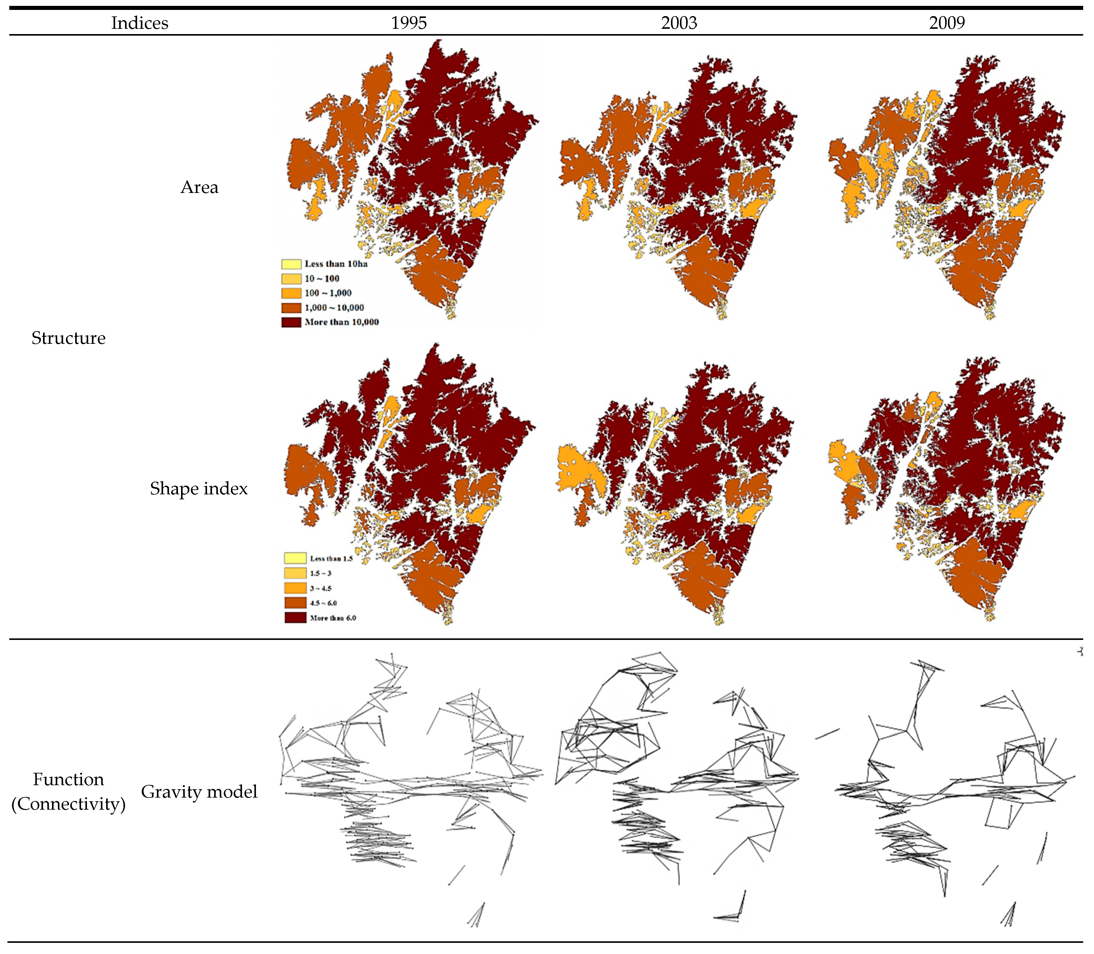
3.1.1. Landscape Structure

Over a fifteen-year period, the total area of landscape patches decreased from 34,978 ha to 31,437 ha and, likewise, the overall number of landscape patches decreased from 2262 to 2132 due to development projects. While both the total number and area of landscape patches has been reduced, the average area has consistently increased because relatively small patches have disappeared due to development projects. Meanwhile, the average shape index has somewhat increased. The lower index (similar to a round shape) is favorable for species’ richness, bio-diversity, and landscape stability [45]. Although the rise of the index is small and the general shape of patches shows no significant change, the increase of the average patch shape index indicates a negative tendency in terms of species’ richness, bio-diversity, and landscape stability. Such a reduction in the total number and area can eventually cause habitat reduction, disturbance of species’ movement, species isolation, and a decrease in habitat biodiversity.

3.1.2. Landscape Function: Connectivity

The connectivity assessment results based on the gravity model revealed that the number of patch networks has decreased by thirteen. Additionally, a 1.6-fold reduction of the gravity index occurred compared with that in 1995. These results were caused by an increase of landscape patch separation distance which is a decrease factor in the gravity index and a relative reduction of the landscape patch area which is an increase factor in the gravity index. The variation of the area and separation distance has also caused changes in the network structure. Meanwhile, connectivity assessment based on least-cost path analysis showed that the friction value of landscape permeability increased by 1.2-fold due to developments. This was the result of land cover changes including agricultural land and forests which are suitable for animal migration that are being transformed into urban built-up areas.

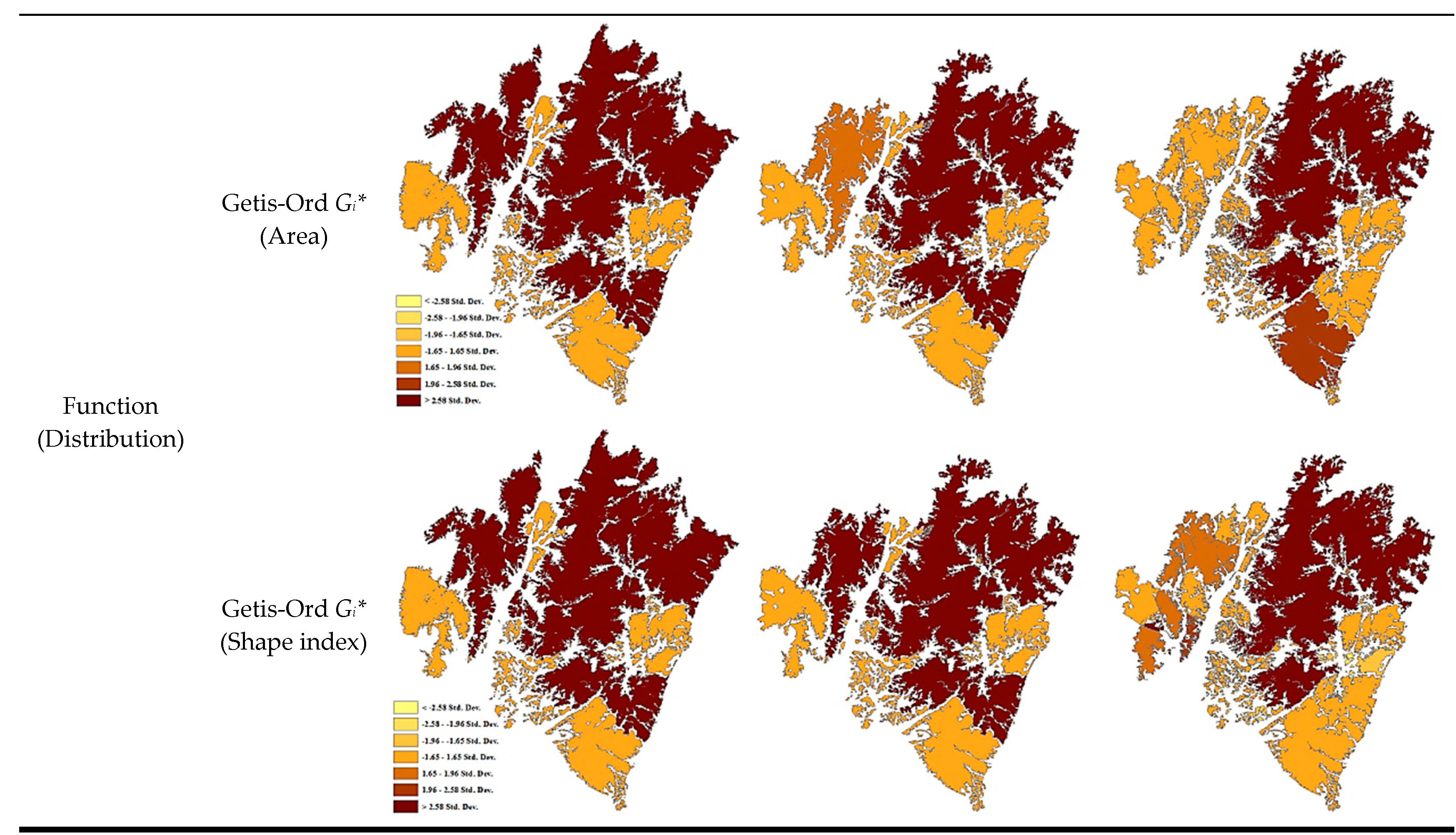
3.1.3. Landscape Function: Distribution

The mean separation distance between landscape patches decreased in time series analysis. Consequently, Global Moran’s I on the area and shape index were estimated as negative values and showed a steady reduction (increasingly negative). This indicates that the distribution of landscape patches has changed to a fragmented and dispersed pattern. Such a landscape patch pattern shows that landscape patch distribution in the study area has changed negatively in terms of bio-diversity and habitant stability. This means that landscape patches identified as hot spots (Z-score > 1.96) or cold spots (Z-score < −1.96) by Getis-Ord G_i* are much larger or much smaller than surrounding patches in terms of area and shape index. Therefore, if landscape patches become hot spots or cold spots, or if the patch pattern of these spots becomes random this would indicate that considerable changes have occurred. Moreover, linear development such as road construction and large housing development has caused a reduction of large landscape patches and variations in their shape and has resulted in changes in the number of both hot and cold spots. Such changes were observed especially in the northwestern and the southern areas of Case Study 1 are of Namyangju. In terms of area, the patch pattern of hot spots in 1985 became random due to a reduction of the patch areas. Subsequently, Getis-Ord G_i* values for the areas of previous hot spots became diversified with varied patch shapes.

3.1.4. Landscape Dynamics: Naturalness

Since the NDVI value is affected by seasonal characteristics, the same season of Landsat imageries were used to calculate NDVI in time series analysis (June 1995; June 2003; June 2009). The NDVI of the study area also decreased in time series analysis. The decreasing amount of NDVI value steeply increased after 1995 when intense developments began in particular. These results were caused by the fact that existing green spaces were changed into developable uses and edge areas of forests were damaged.

3.1.5. Comprehensive Assessment Results of Case Study 1

As development continuously occurred in the study area, the pattern of landscape patch distribution and connectivity has changed negatively with structural variations including a decrease in the number of landscape patches, area reduction, and shape changes. Land cover was changed from agricultural to urban use and as a result, road networks increased. Consequently, the network structure changed from a circulation to a linear branch shape because suitable patch areas for connectivity were not secured. Thus, as a negative variation for species richness has been occurring, landscape ecological values in the study area has been decreasing over the last twenty years.

Such negative variations were identified clearly near the development projects. From Case Study 1, locations and the amount of variations of the landscape were identified accurately and quantitatively using time series analysis. More effective landscape management to enhance landscape ecological value can be developed by focusing on areas of connectivity decrease and on hot or cold spot areas (Figure 6 and

Table 7. Integrated assessment results (Case Study 1).

Indices			1995	2003	2009
Structure	The number of landscape patches		2862	2266	2132
	Area	Total area (ha)	34,978	33,637	31,437
		Mean area (ha)	10.64	13.50	14.08
	Mean shape index		1.31	1.33	1.34
Function (Connectivity)	Gravity model	The number of networks	50	42	37
		Mean gravity index	20,121,716	14,783,855	12,371,455
	Landscape permeability		2,069,640	2,483,568	2,657,417
Function (Distribution)	Mean separation distance (m)		126.57	150.52	171.43
	Area (Moran’s I)		−0.61	−0.66	−0.71
	Shape index (Moran’s I)		0.00	−0.01	−0.02
	Area (Getis-Ord Gi*)	The number of hot spots	8	8	9
		The number of cold spots	6	7	9
	Shape index (Getis-Ord Gi*)	The number of hot spots	13	14	14
		The number of cold spots	8	8	12
Dynamics (Naturalness)	Mean NDVI		198	184	156

).

3.2. Results of Case Study 2

3.2.1. Landscape Structure: Area and Shape

For landscape structure, the number of patches increased from 19 to 135 particularly in terms of the original development plan. The total landscape patch area also increased from 10,551.45 ha to 10,569.14 ha. However, the mean area decreased by 477.05 ha. This is due to the fact that landscape patches including parks, corridors, and green buffers were planned with various shapes and areas. Meanwhile, in the improved development plan the total number of landscape patches decreased to 66 from 135 because the separated landscape patches were integrated in order to enhance connectivity between landscape patches. The total area also increased to 10,688.09 ha, and the mean area rose by 83.66 ha in relation to the original development plan while the shape index decreased from 2.67 to 2.35. This means that the improved development plan is more favorable for species’ habitation than the existing plan in terms of landscape patch shape. Moreover, as the shape index of the improved plan decreased even more by 2.21 and the improved development plan turned out to be more suitable than the original development plan.

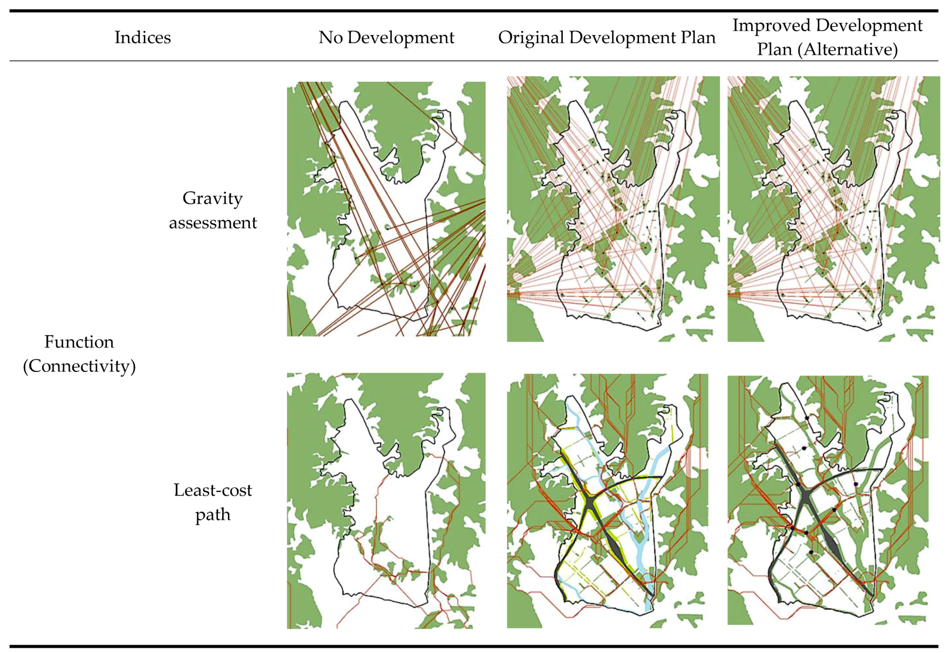
3.2.2. Landscape Function: Connectivity

The connectivity assessment results based on the gravity model (Figure 7) showed that the number of patch networks increased threefold by the original development plan. However, a threefold decrease of the gravity index occurred due to the development plan. This result was due to the fact that individual patch areas were not sufficiently secured by inner road networks although the separation distance of the landscape patches decreased. In the case of the improved development plan, however, connectivity was enhanced compared with the original development plan, as the number of connecting networks decreased about two-fold, and a two-fold increase of the gravity index occurred. As patches were connected by the improved plan, individual patch areas were sufficiently secured and the separation distance decreased. Meanwhile, the connectivity assessment results regarding landscape showed that the friction value increased by eighteen-fold as a result of urban development. This was the result of land cover changes from agricultural land which is suitable for animal migration to the urban developed area after development. The improved plan showed slight enhancement compared with the original development plan because additional green spaces were secured.

3.2.3. Landscape Function: Distribution

The mean separation distance of patches decreased from 3269 m to 1569 m in terms of the original development plan. In the case of the improved development plan, the average separation distance present was 1369 m which is a decrease by 200 m compared with the original development plan. This means that the separation distance of the improved plan is most suitable considering the number of landscape patches and area.

Meanwhile, regional distribution of landscape patches based on area shows that some fragmentation has occurred after urban development as Global Moran’s I decreased from 0.11 to 0.01. In the improved development plan, the distribution pattern was enhanced somewhat as Global Moran’s I increased about 0.02. However, in terms of shape index, the improved plan showed the lowest of Global Moran’s I. This result was caused by landscape patches being changed into various shapes due to the improved plan which integrated separated landscape patches.

In the case of Getis-Ord G_i* on area, the number of hot spots increased by 1 in the original development plan. This result was due to the fact that the landscape patches near the study area became relatively larger compared with the inner patches which were fragmented into small ones by the development plan. Furthermore, the number of hot spot areas in the improved plan was equal to that of the original development plan. Through the Getis-Ord G_i* assessment on shape index, the number of hot spot areas increased by 3 as landscape patches fragmented and changed into various shapes by the original development plan. However, compared with the original development plan, enhancement of the distribution was found in the improved plan because the number of hot spots decreased to 1.

3.2.4. Comprehensive Assessment Results of Case Study 2

Landscape ecological performance due to the new town project has resulted in positive effects such as patch number increase, total area increase, and fragmentation improvement in the study area. However, landscape ecological performance that includes shape and connectivity was found to have changed negatively due to sufficient areas not being secured as land cover changed from agricultural land into an urban area and because road networks increased. Therefore, if the fragmented areas are minimized by establishing an underground road, eco-bridge, etc., connectivity can be enhanced in the study area. The integrated assessment results of the improved plan which introduced additional green infrastructure to connect fragmented patches show that most assessment indices (area, shape, gravity index, landscape permeability) of the improved plan becomes more favorable than the original development plan except for Getis-Ord G_i* based on patch area and network number.

For structure, the number of landscape patches decreased as separated patches were connected but more stability was achieved as total area increased. As landscape patch shape also changed into a round configuration, the improved plan was found to be more suitable for conserving natural resources. In addition, when integrating fragmented patches caused a reduction in the separation distance and clustering landscape patches, landscape ecological performances were enhanced in Global Moran’s I based on area and Getis-Ord G_i* which, in turn, was based on shape index.

In the case of connectivity, as the number of landscape patches decreased the number of networks also reduced but the gravity index increased considerably because additional patch areas were provided and the separation distance lessened. For the connectivity assessment results by least-cost path analysis, connectivity was enhanced a little compared with the original development plan as friction value decreased somewhat due to additional green infrastructure provision (

Table 8. Integrated assessment results.

Indices			No Development	Original Development Plan	Improved Development Plan (Alternative)
Structure	The number of landscape patches		19	135	66
	Area	Total area (ha)	10,551.45	10,569.14	10,688.09
		Average area (ha)	555.33	78.28	161.94
	Mean shape index		2.67	2.35	2.21
Function (Connectivity)	Gravity model	The number of networks	19	53	25
		Mean gravity index	3,133,191	1,019,344	2,184,376
	Landscape permeability		22,996	425,537	423,386
Function (Distribution)	Mean separation distance (m)		3269	1569	1369
	Area (Moran’s I)		0.11	0.01	0.03
	Shape index (Moran’s I)		0.17	0.04	0.00
	Area (Getis-Ord Gi*)	The number of hot spots	1	2	2
		The number of cold spots	0	0	0
	Shape index (Getis-Ord Gi*)	The number of hot spots	1	4	1
		The number of cold spots	0	0	0

). Synthetically, the integrated assessment results clearly show that the improved development plan is more favorable in terms of landscape ecological performance than the original development plan.

3.3. The Differences of GIAS Compare to Other Systems

Through the case studies, the differences of GIAS compared with other systems (FRAGSTAT, Patch analyst, V-Late, and LCM) were identified. Those differences are as follows: First, while the main purpose of the other systems is to analyze landscape ecological indices, GIAS has been developed to focus on its use as a green infrastructure planning support tool. In this regard, the evaluation process of GIAS was prepared to link the entire process of spatial planning.

Second, while other systems have only quantitatively derived connectivity and distribution assessment results, GIAS can provide both quantitative results and maps from the gravity model, the least-cost path analysis, and Getis ord Gi* analysis. Such visualization of analysis results have advantages in connectivity and distribution analysis compared to other systems. In the case of other systems, only the intensity of connectivity was analyzed quantitatively, so there was a limit in determining which locations in the study area were strong or weak. In the analysis of distribution, it was difficult to visually identify the cluster pattern because the existing system mainly provided the distance and isolation analysis results only in numerical values. The evaluation by GIAS are derived by spreadsheets and maps, so that the evaluation results can be more effectively comprehended.

Third, the system is applicable to both the macro scale and micro scale. The success of green infrastructure planning and management depends on the congruence between the operational scales of green infrastructure and the spatial scope of the planning instruments [50]. However, other systems have been mainly applied to macro scale analysis because they utilize landscape patches which were extracted from satellite images.

Finally, GIAS was developed to help non-experts of landscape ecology and GIS. The integrated assessment function was developed for effective assessment, and it has the advantage of considering multiscale approaches in landscape indices analysis. The other systems also have integrated assessment capabilities, but both patch level and class level analysis are performed separately. Therefore, it was difficult to identify the interrelationship between landscape indices. In case of GIAS, the interrelationship between landscape indices (e.g., structure and function) could be more easily identified because patch level analysis and class level analysis are performed sequentially by integrated assessment. Furthermore, both of the other systems require repetitive project file creation for time series analysis or alternative comparisons. In the case of GIAS, if landscape patch data are prepared by time series or alternatives, comparisons are possible to be performed without separate project file creation. In addition, other systems mainly use one kind of analysis (raster-based or vector based), but GIAS improves user’s convenience by using both raster and vector formats.

4. Discussion

On the macro scale, the landscape patch changes due to development projects have been observed quantitatively, and their results were also mapped. Similar to previous studies, the results confirmed that the ecological value of landscape patches is decreasing by development projects. With the reduction of the landscape patches, the relatively strong landscape network structure has been weakening. In addition, results of Getis Ord Gi* confirmed that drastic landscape variations have occurred near the development projects. Mapping transformations taking place in the landscape and determining the forces causing them is essential for landscape change monitoring [29]. In fact, there have been few studies to analyze the structural changes of connectivity and distribution according to development projects. As a result, GIAS can be employed to identify and visualize changed landscape ecological values on the macro scale caused by negative driving forces (large urban developments, road construction etc.) through assessments of structure, function, and dynamics of the landscape. In restoration planning, decision makers can focus on primary areas for restoration as well as areas for conservation based on the GIAS’ assessment results. Furthermore, landscape ecological values that are the result of specific green infrastructure plans can be monitored after the completion of a development project.

On the other hand, GIAS enables more effective decision support to be rendered even on a micro scale through quantitative and spatial comparison of various alternatives in spatial planning. The locations where additional corridors for enhancing connectivity should be introduced in the urban development project area were clearly delineated by GIAS. Moreover, as presented in

Table 9. Comparison GIAS with other systems.

	FRAGSTATS	LCM (Land Change Modeler)	Patch Analyst	V-LATE (Vector-Based Landscape Analysis Tools)	GIAS
Main Usage	Landscape ecological indices assessment	Analysis of landscapes change according to future land use change	Landscape ecological indices assessment	Landscape ecological indices assessment	Spatial planning decision support
Analytical scale	Micro and macro (Mainly macro)	Macro	Macro and micro (Mainly macro)	Macro and micro	Macro and micro
Connectivity and distribution assessment results	Only quantitative results	None	Only quantitative results	Only quantitative results	Quantitative results maps from network gravity model and the least-cost path analysis
Alternative or time series comparison (Integrated assessment)	Needs a separate project file for each alternative or time series for comparison	Able to compare within a single project file	Needs a separate project file for each alternative or time series for comparison	Needs a separate project file for each alternative or time series for comparison	Able to compare within a single project file
Analysis data format	Only raster	Only raster	Mainly vector	Only vector	Vector and raster
Result identification and visualization	Only spreadsheet	Spreadsheet and maps	Spreadsheet and maps (Need GIS software to identify maps)	Spreadsheet and maps (Need GIS software to identify maps)	Spreadsheet and map

, structural and functional variations due to small landscape changes were also measured. Alternative assessments on green infrastructure have tended to be mainly conducted by planner professional intuition or through surveyed opinions. As presented in the results of case study 2, the assessment methods developed in this study can aid in the investigation of landscape ecological performance intrinsic in the development plan to be more detailed and concrete.

In assessing landscape patches, patch level analysis has the advantage of investigating individual structure (area, shape) of landscape patches. However, it is difficult to investigate landscape functions (connectivity and distribution) because they are determined by the interrelationship of individual patches. On the other hand, class level analysis is useful to investigate the overall structure of landscape patches. Thus, multilevel approaches are required for in-depth analysis of the structure-function-dynamics of landscape patches. In this regard, the integrated assessment was developed to consider patch level as well as class level. As presented in Table 8 and Table 9, the variation of landscape indices is clearly identified. In particular, the connectivity which is a key concept of green infrastructure is clearly estimated. Thus, as a tool for evaluating values of landscape patches, the usefulness of the integrated assessment by GIAS was explained.

5. Conclusions

This study established GIAS to enhance landscape ecological values of urban spaces. The applicability and usefulness of GIAS were investigated through case studies and the study results clearly demonstrate that concrete assessment of landscape ecological values both on the macro and micro scale can be achieved. In addition, human-induced impacts on the landscape resulting from diverse development projects that frequently occur can be examined in advance and alternatives to reduce their adverse impacts can be developed proactively. As such, GIAS can be applied to all stages in spatial planning. For example, at an initial survey stage, areas for primary conservation and restoration can be delineated based on the naturalness assessment and the bio-diversity assessment results prior to planning, and desired ecological value goals can be identified. At the schematic planning stage, a desirable ecological goal of a spatial plan and project can be achieved through structure assessment results and an enhanced spatial structure of the site considering ecological networks can be prepared using the connectivity assessment results. In developing detailed plans, an effective arrangement and networking of green infrastructure to enhance ecological stability can be simulated and evaluated by diverse functions embedded in GIAS. These networking assessment results achieve the goal of green infrastructure planning, i.e., networking green infrastructure resources. As a result, GIAS can be utilized as an effective decision-making tool for scientific and systematic planning and management of green infrastructure.

Improvements to further develop GIAS are as follows: First, the effectiveness of the bio-diversity index was not investigated in this study due to a lack of time series data. Second, since this study utilized a 30 m × 30 m spatial resolution land cover map as raw data, NDVI was analyzed by using a Landsat satellite image with the same resolution. Recent developments in remote sensing technology have made it possible to acquire higher resolution NDVIs. Therefore, if the NDVI analysis uses higher resolution satellite images in GIAS, more accurate monitoring of green infrastructure will be possible. Third, comprehensive consideration of human-social elements such as population, land use, and infrastructure to create ecological planning is required. If other benefits like landscape perception, recreation, and human health are verified with ecological value, the usefulness of GIAS will be more definable.

References

1. Forman, R.T.T.; Godron, M. Landscape Ecology; John Wiley & Sons: New York, NY, USA, 1986. [Google Scholar]
2. Steiner, F.R. The Living Landscape: An Ecological Approach to Landscape Planning; McGraw-Hill: New York, NY, USA, 2000. [Google Scholar]
3. Termorshuizen, J.W.; Opdam, P. Landscape services as a bridge between landscape ecology and sustainable development. Landsc. Ecol. 2009, 24, 1037–1052. [Google Scholar] [CrossRef]
4. Turner, M.G.; Gardner, R.H.; O’neill, R.V. Landscape Ecology in Theory and Practice: Pattern and Process; Springer: New York, NY, USA, 2015. [Google Scholar]
5. Adriaensen, F.; Chardon, J.P.; De Blust, G.; Swinnen, E.; Villalba, S.; Gulinck, H.; Matthysen, E. The application of ‘least-cost’ modelling as a functional landscape model. Landsc. Urban Plan. 2003, 64, 233–247. [Google Scholar] [CrossRef]
6. Hawkins, V.; Selman, P. Landscape scale planning: exploring alternative land use scenarios. Landsc. Urban Plan. 2002, 60, 211–224. [Google Scholar] [CrossRef]
7. Lienert, J. Habitat fragmentation effects on fitness of plant populations—A review. J. Nat. Conserv. 2004, 12, 53–72. [Google Scholar] [CrossRef]
8. Olsen, L.M.; Dale, V.H.; Foster, T. Landscape patterns as indicators of ecological change at Fort Benning, Georgia, USA. Landsc. Urban Plan. 2007, 79, 137–149. [Google Scholar] [CrossRef]
9. Moran, P.A.P. Notes on Continuous Stochastic Phenomena. Biometrika 1950, 37, 17–23. [Google Scholar] [CrossRef] [PubMed]
10. Reynolds, K.M.; Hessburg, P.F. Decision support for integrated landscape evaluation and restoration planning. For. Ecol. Manag. 2005, 207, 263–278. [Google Scholar] [CrossRef]
11. Zhang, L.; Wang, H. Planning an ecological network of Xiamen Island (China) using landscape metrics and network analysis. Landsc. Urban Plan. 2006, 78, 449–456. [Google Scholar] [CrossRef]
12. Mörtberg, U.M.; Balfors, B.; Knol, W.C. Landscape ecological assessment: A tool for integrating biodiversity issues in strategic environmental assessment and planning. J. Environ. Manag. 2007, 82, 457–470. [Google Scholar] [CrossRef]
13. Cook, E.A. Landscape structure indices for assessing urban ecological networks. Landsc. Urban Plan. 2002, 58, 269–280. [Google Scholar] [CrossRef]
14. Kong, F.; Yin, H.; Nakagoshi, N.; Zong, Y. Urban green space network development for biodiversity conservation: Identification based on graph theory and gravity modeling. Landsc. Urban Plan. 2010, 95, 16–27. [Google Scholar] [CrossRef]
15. Oh, K.; Lee, D.; Park, C. Urban Ecological Network Planning for Sustainable Landscape Management. J. Urban Technol. 2011, 18, 39–59. [Google Scholar] [CrossRef]
16. Benedict, M.A.; MacMahon, E.T. Green infrastructure: Smart conservation for the 21st century. Renew. Resour. J. 2002, 20, 12–17. [Google Scholar]
17. Liquete, C.; Kleeschulte, S.; Dige, G.; Maes, J.; Grizzetti, B.; Olah, B.; Zulian, G. Mapping green infrastructure based on ecosystem services and ecological networks: A Pan-European case study. Environ. Sci. Policy 2015, 54, 268–280. [Google Scholar] [CrossRef]
18. Zhang, Z.; Meerow, S.; Newell, J.P.; Lindquist, M. Enhancing landscape connectivity through multifunctional green infrastructure corridor modeling and design. Urban For. Urban Green. 2019, 38, 305–317. [Google Scholar] [CrossRef]
19. Lee, J.; Chon, J.; Ahn, C. Planning Landscape Corridors in Ecological Infrastructure Using Least-Cost Path Methods Based on the Value of Ecosystem Services. Sustainability 2014, 6, 7564–7585. [Google Scholar] [CrossRef] [Green Version]
20. Kienast, F.; Frick, J.; van Strien, M.J.; Hunziker, M. The Swiss Landscape Monitoring Program–A comprehensive indicator set to measure landscape change. Ecol. Model. 2015, 295, 136–150. [Google Scholar] [CrossRef]
21. Krajewski, P. Monitoring of Landscape Transformations within Landscape Parks in Poland in the 21st Century. Sustainability 2019, 11, 2410. [Google Scholar] [CrossRef]
22. Bürgi, M.; Bieling, C.; von Hackwitz, K.; Kizos, T.; Lieskovský, J.; Martín, M.G.; McCarthy, S.; Müller, M.; Palang, H.; Plieninger, T.; et al. Processes and driving forces in changing cultural landscapes across Europe. Landsc. Ecol. 2017, 32, 2097–2112. [Google Scholar] [CrossRef] [Green Version]
23. Kumar, M.; Denis, D.M.; Singh, S.K.; Szabó, S.; Suryavanshi, S. Landscape metrics for assessment of land cover change and fragmentation of a heterogeneous watershed. Remote. Sens. Appl. Soc. Environ. 2018, 10, 224–233. [Google Scholar] [CrossRef] [Green Version]
24. Kubacka, M. Evaluation of the ecological efficiency of landscape protection in areas of different protection status. A case study from Poland. Landsc. Res. 2018, 1–14. [Google Scholar] [CrossRef]
25. Szabó, P. Driving forces of stability and change in woodland structure: A case-study from the Czech lowlands. For. Ecol. Manag. 2010, 259, 650–656. [Google Scholar] [CrossRef]
26. Seabrook, L.; McAlpine, C.; Fensham, R. Cattle, crops and clearing: Regional drivers of landscape change in the Brigalow Belt, Queensland, Australia, 1840–2004. Landsc. Urban Plan. 2006, 78, 373–385. [Google Scholar] [CrossRef]
27. Zewdie, M.; Worku, H.; Bantider, A. Temporal Dynamics of the Driving Factors of Urban Landscape Change of Addis Ababa During the Past Three Decades. Environ. Manag. 2018, 61, 132–146. [Google Scholar] [CrossRef] [PubMed]
28. Krajewski, P.; Solecka, I.; Mrozik, K. Forest Landscape Change and Preliminary Study on Its Driving Forces in Ślęża Landscape Park (Southwestern Poland) in 1883–2013. Sustainability 2018, 10, 4526. [Google Scholar] [CrossRef]
29. Krajewski, P. Assessing Change in a High-Value Landscape: Case Study of the Municipality of Sobotka, Poland. Pol. J. Environ. Stud. 2017, 26, 2603–2610. [Google Scholar] [CrossRef]
30. Lee, D.; Oh, K. A Landscape Ecological Management System for Sustainable Urban Development. APCBEE Procedia 2012, 1, 375–380. [Google Scholar] [CrossRef] [Green Version]
31. Do, D.T.; Huang, J.; Cheng, Y.; Truong, T.C.T. Da Nang Green Space System Planning: An Ecology Landscape Approach. Sustainability 2018, 10, 3506. [Google Scholar] [CrossRef]
32. Gurrutxaga, M.; Lozano, P.J.; del Barrio, G. GIS-based approach for incorporating the connectivity of ecological networks into regional planning. J. Nat. Conserv. 2010, 18, 318–326. [Google Scholar] [CrossRef]
33. Wu, J. Urban sustainability: an inevitable goal of landscape research. Landsc. Ecol. 2010, 25, 1–4. [Google Scholar] [CrossRef]
34. Opdam, P.; Foppen, R.; Vos, C. Bridging the gap between ecology and spatial planning in landscape ecology. Landsc. Ecol. 2001, 16, 767–779. [Google Scholar] [CrossRef]
35. Naveh, Z. What is holistic landscape ecology? A conceptual introduction. Landsc. Urban Plan. 2000, 50, 7–26. [Google Scholar] [CrossRef]
36. Norton, B.A.; Evans, K.L.; Warren, P.H. Urban Biodiversity and Landscape Ecology: Patterns, Processes and Planning. Curr. Landsc. Ecol. Rep. 2016, 1, 178–192. [Google Scholar] [CrossRef] [Green Version]
37. McGarigal, K.; Marks, B.J. FRAGSTATS: Spatial Pattern Analysis Program for Quantifying Landscape Structure; Gen. Tech. Rep. PNW-GTR-351; U.S. Department of Agriculture, Forest Service Pacific Northwest Research Station: Corvallis, OR, USA, 1995.
38. Forman, R.T.T. Some general principles of landscape and regional ecology. Landsc. Ecol. 1995, 10, 133–142. [Google Scholar] [CrossRef]
39. Kim, H.; Oh, K.; Lee, D.K. A Time-Series Analysis of Landscape Structural Changes using the Spatial Autocorrelation Method-Focusing on Namyangju Area. J. Korea Soc. Environ. Restor. Technol. 2011, 14, 1–14. [Google Scholar]
40. Knaapen, J.P.; Scheffer, M.; Harms, B. Estimating habitat isolation in landscape planning. Landsc. Urban Plan. 1992, 23, 1–16. [Google Scholar] [CrossRef]
41. Ignatieva, M.; Stewart, G.H.; Meurk, C. Planning and design of ecological networks in urban areas. Landsc. Ecol. Eng. 2011, 7, 17–25. [Google Scholar] [CrossRef]
42. Botequilha Leitão, A.; Ahern, J. Applying landscape ecological concepts and metrics in sustainable landscape planning. Landsc. Urban Plan. 2002, 59, 65–93. [Google Scholar] [CrossRef]
43. Ramalho, C.E.; Hobbs, R.J. Time for a change: Dynamic urban ecology. Trends Ecol. Evol. 2012, 27, 179–188. [Google Scholar] [CrossRef]
44. Schonewald-Cox, C.; Chambers, S.; MacBryde, B.; Thomas, L. Guidelines to management: A beginning attempt. In Genetics and Conservation; Benjamin Cummings Publ. Co.: Menlo Park, CA, USA, 1983; pp. 414–445. [Google Scholar]
45. Dramstad, W.E.; Olson, J.D.; Forman, R.T.T. Landscape Ecology Principles in Landscape Architecture and Land-Use Planning; Island Press: Washington, DC, USA, 1996. [Google Scholar]
46. Getis, A.; Ord, J.K. The Analysis of Spatial Association by Use of Distance Statistics. Geogr. Anal. 1992, 24, 189–206. [Google Scholar] [CrossRef]
47. Luck, G.W.; Daily, G.C.; Ehrlich, P.R. Population diversity and ecosystem services. Trends Ecol. Evol. 2003, 18, 331–336. [Google Scholar] [CrossRef] [Green Version]
48. Opdam, P.; Steingröver, E.; Rooij, S.V. Ecological networks: A spatial concept for multi-actor planning of sustainable landscapes. Landsc.Urban Plan. 2006, 75, 322–332. [Google Scholar] [CrossRef]
49. Bürgi, M.; Hersperger, A.M.; Schneeberger, N. Driving forces of landscape change—Current and new directions. Landsc. Ecol. 2004, 19, 857–868. [Google Scholar] [CrossRef]
50. Niedźwiecka-Filipiak, I.; Rubaszek, J.; Potyrała, J.; Filipiak, P. The Method of Planning Green Infrastructure System with the Use of Landscape-Functional Units (Method LaFU) and its Implementation in the Wrocław Functional Area (Poland). Sustainability 2019, 11, 394. [Google Scholar]
Figure 1. The main functions of the Green Infrastructure Assessment System (GIAS).
Sustainability 11 03798 g001
Figure 2. The case study area.
Sustainability 11 03798 g002
Figure 3. The three stages for assessment.
Sustainability 11 03798 g003
Figure 4. Development projects in Study Area 1.
Sustainability 11 03798 g004
Figure 5. Land cover changes in Study Area 1 (1995, 2003, and 2009).
Sustainability 11 03798 g005
Figure 6. Assessment results by GIAS (Case Study 1).
Sustainability 11 03798 g006aSustainability 11 03798 g006b
Figure 7. Assessment results by GIAS (Case Study 2).
Sustainability 11 03798 g007