Article

Spectral Deconvolution for Dimension Reduction and Differentiation of Seagrasses: Case Study of Gulf St. Vincent, South Australia

1
Department of Environmental Engineering, National Cheng Kung Chung University, Tainan 701, Taiwan
2
Global Water Quality Research Center, National Cheng Kung University, Tainan 701, Taiwan
3
Department of Ecology and Evolutionary Biology, The University of Adelaide, Adelaide, South Australia 5005, Australia
4
Australian Water Quality Centre, SA Water, Adelaide, South Australia 5000, Australia
5
College of Science and Engineering, Flinders University, Adelaide, South Australia 5001, Australia
*
Authors to whom correspondence should be addressed.
Sustainability 2019, 11(13), 3695; https://doi.org/10.3390/su11133695
Submission received: 30 May 2019 / Revised: 1 July 2019 / Accepted: 1 July 2019 / Published: 5 July 2019

Abstract

:
Seagrasses are a vulnerable and declining coastal habitat, which provide shelter and substrate for aquatic microbiota, invertebrates, and fishes. More accurate mapping of seagrasses is imperative for their sustainability but is hindered by the lack of data on reflectance spectra representing the optical signatures of individual species. Objectives of this study are: (1) To determine distinct characteristics of spectral profiles for sand versus three temperate seagrasses (Posidonia, Amphibolis, and Heterozostera); (2) to evaluate the most efficient derivative analysis method of spectral reflectance profiles for determining benthic types; and to assess the influences of (3) site location and (4) the water column on spectral responses. Results show that 566:689 and 566:600 bandwidth ratios are useful in separating seagrasses from sand and from detritus and algae, respectively; first-derivative reflectance spectra generally is the most efficient method, especially with deconvolution analyses further helping to reveal and isolate 11 key wavelength dimensions; and differences between sites and water column composition, which can include suspended particulate matter, both have no effect on endmembers. These findings helped develop a spectral reflectance library that can be used as an endmember reference for remote sensing, thereby providing continued monitoring, assessment, and management of seagrasses.

1. Introduction

Seagrasses are angiosperms (flowering plants) that can form dense beds within shallow, soft-benthic marine and estuarine environments [1,2,3]. In doing so, they function as a substrate and shelter for epiphytic algae as well as invertebrates and fishes, further contributing to the biodiversity and productivity of a coastal ecosystem [1,3,4,5,6,7,8]. Because of this, such aquatic environments also provide valuable services for humans through the fisheries and aquaculture industries [4,9,10] as well as allow for recreational activities such as tourism [4,9,11]. Seagrasses are thus a vital coastal habitat worldwide and are increasingly vulnerable to anthropogenic impacts. Seagrasses are in decline; with 29% of known seagrass areal extent being lost since 1879 [12,13]. The situation is similar in metropolitan coastal waters of South Australia [14], a region that experienced a loss of 85 ha yr −1 on average until the early 2010s [15,16], with a slow come back in the last decade, highlighting the need for more accurate mapping of seagrasses [17,18,19] in the area.
Baseline knowledge as well as continual monitoring of seagrass distribution is increasingly crucial to mitigate any further losses, because it identifies areas suitable for sustainable protection [4,20,21]. Traditionally, mapping of seagrass and other benthic bottom types has utilized boat- and land-based surveys, both of which are limited by cost and time to effectively cover expansive and inaccessible areas [20,22]. Remote sensing has become a useful alternative, particularly due to advances in spaceborne and airborne detection sensors [2,23,24,25,26,27]. Spectral imaging remote sensing has proven to be a useful tool, regardless of whether spectral imaging is passive with very high spectral resolution over contiguous bands (hyperspectral), or active with lower spectral resolution in discrete narrow bandwidths (multispectral) [28,29]. This is so because its reflectance responses vary along the light spectrum, often providing distinct optical signatures that can be repeatedly measured to provide multi-dimensional information [2,25,28,30,31]. In addition, underwater communities can only be detected with wavelengths in the visible light spectrum (≈350–750 nm), where light can penetrate the water column without being easily absorbed and get reflected to the sensor [5,24,32]. However, while remote sensing is a useful tool for detecting changes in benthic cover, effective application of such technology necessitates appropriate dimension and component reduction as well as concrete understanding of the spectral behaviors of benthic substrates.
Using a system analysis approach, the goal of detecting and improving the monitoring of seagrasses can be defined in simpler relationships [33,34] with fewer dimensions and components needing to be analyzed [25,27]. Specifically, only if the spectral properties of a particular seagrass are distinct and not spectrally confused with the surrounding benthic bottom cover types such as sand, epiphytes, macroalgae, and detritus, can it then be detected through remote sensing [21,22,31,32,35]. Because of this, a library of benthic bottom type spectra profiles should be established a priori so its profiles can be referenced as endmembers during multispectral or hyperspectral remote sensing [14,22,36,37]. Useful and applicable extraction of remote sensing data relies on the detection of even slight variations within the spectral wavelength dimensions, specifically at particular bandwidths [21,27,38]. These slight variations can be assessed through various techniques, which include calculating bandwidth ratio slopes of reflectance features [21,39,40,41,42] and calculating derivative curves [21,37,41,42,43,44,45,46,47,48,49].
Major regions representing the spectral shape such as the UV-visible light, acute green, and red edge regions help to best differentiate slight variations between reflectance profiles [5,50], although the choice of a particular number of non-contiguous wavebands for separation of benthic bottom type is specific to in situ reflectance of a study site [45]. In particular, reflectance ratios of the green peak-to-descending edge (566:600 nm) and green peak-to-near infrared NIR peak of sand (566:694 nm) have been reported as effective tools for separating benthic substrates, especially since these ratios are based on spectral shape rather than magnitude [21]. Additionally, derivative analyses of hyperspectral data have been used in many studies to identify not so obvious peak features. This helps minimize the number of key bandwidths. However, the efficiency of first-, second, and fourth-derivatives remains in question. Some authors steadily relied solely on the first order derivatives [21,37,46,49], while others also utilized second- and fourth-order derivatives [45,47,48,51]. By utilizing bandwidth ratios to identify unique markers within the reflectance profile as well as analyzing derivatives of these profiles, the number of relevant wavelength dimensions may be reduced.
Derivative analyses provide a pathway to identify statistically significant spectral differences between benthic bottom types. Other classic approaches include cluster analysis, principal components analysis, and discriminant function analysis [23,45,49,52]. Because these methods, however, describe the separability in terms of linear functions [53] based on multiple variables rather than a specific reflectance wavelength and amplitude, there has been a call for more rigorous statistical approaches [54,55]. The deconvolution technique is another useful tool often used in other scientific disciplines to reveal peaks in poorly resolved spectra [56,57,58]. The technique involves deconvolving spectrally mixed signals by resolving a convolution function and identifying multiple peaks along the light spectrum that comprise and contribute to the spectral profile. Spectral derivative profiles can be combined with deconvolution analyses to help further characterize unique peaks in benthic bottom types [47], thereby further reducing the number of potential spectral dimensions that need to be studied.
This study applies the bandwidth ratios, derivative, and deconvolution analysis to develop and refine spectral signature profiles characteristic of bare sand and three temperate seagrasses (Posidonia, Amphibolis, and Heterozostera). The objectives are: (1) To identify unique characteristics of spectral profiles for each benthic bottom type; (2) to analyze the most efficient analysis method of spectral reflectance profiles used for determining dominant seagrasses within the coastal waters; and to assess the influences of (3) site location and (4) the water column on the spectral reflectance responses.

2. Materials and Methods

2.1. Study Area

The two study sites, Bolivar and Seacliff, were located north and south along the optically shallow coasts of metropolitan-Adelaide, respectively (Figure 1). These two sites are located in Gulf St. Vincent, South Australia. At the Bolivar site (34°42′55.82”S, 138°26′45.57”E), which is located about 1 km northwest of the outfall for Bolivar Wastewater Treatment Plant, Posidonia is the dominant seagrass accompanied by a less dense cover of Heterozostera [59,60]. Despite losses in the area [61], the distribution of Posidonia and Heterozostera spp. in the northern site remains consistent nearly a decade later [18]. Within the Seacliff site (35°2′12.05”S, 138°30′37.19”E), which is located about 0.5 km west of Seacliff Beach, both algae and Amphibolis seagrass are considered major features specific to this zone [60,62], with Posidonia followed by Amphibolis as the dominant seagrass taxa usually occurring in monotypic meadows [63]. Because of higher wave energy associated with the southern region [64], the distribution of Posidonia throughout the Seacliff site is more fragmented than the northern region [63].

2.2. Field Sampling

Spectral responses for dominant benthic bottom types—Posidonia, Amphibolis, Heterozostera seagrasses, and sand—were sampled approximately every 15 days, weather permitting, at the Bolivar and Seacliff study sites during the summer months (December 2015–January 2016). Multiple sites were sampled within these two locations (Figure 1). Snorkeling was used for surveying the specimens; samples were collected from the seafloor by hand and brought onto the boat. Samples of each seagrass species were collected from areas of seagrass known to grow principally in homogeneous (monospecific) patches. Collected bottom type samples were sorted by seagrass taxa and genera; additionally, samples of sand were taken during each sampling date. In situ downwelling underwater irradiance (Ed- in-situ) was measured using a cosine corrector sensor each time latitude/longitude was changed.

2.3. Measuring Reflectance Spectra of Benthic Types

Benthic samples collected in the field were taken to an outdoor laboratory managed by the Australian Water Quality Centre to measure for spectral reflectance on cloud-free days within 3 h of solar noon, wherever possible. Samples were placed in an open air 12 L hydraulic vessel, with the interior of the vessel lined in black [45] to minimize wall effects of light field [23,45,65]. The vessel was filled with marine water to a height of 10 cm.
A subset of uneven sample sizes for each seagrass genera was measured using vacuum filtered marine water (Whatman GF/C 1.2 μm glass microfiber filter, 90 mm diameter). Reflectance measurements for each benthic bottom type consisted of using a JAZ-2 spectroradiometer [66] sensor with an attached cosine corrector to measure both upwelling underwater radiance of a particular benthic bottom type (Eu- benthic) and its related underwater baseline radiance (Eu- base). The sensor contains a collecting tip with a fiber optic cable (3 m long, 400 μm diameter) that transmits light, and was mounted to a non-reflective black-colored pole placed just beneath the water surface, pointed at an angle of ~45° nadir from the specimen sample to record radiance (≈190–890 nm).
Each sample was averaged for more than 200 spectra with an integration time of 10 microseconds; signal-to-noise ratio (SNR) was reported at 250:1 [67].
Reflectance R was calculated using the following equation:
R b e n t h i c   =   ( E u . b e n t h i c ) ( E u . b a s e ) E d . i n s i t u
where three main components were measured: upwelling underwater radiance of a particular benthic bottom type (Eu-benthic); upwelling underwater radiance of a baseline, in this case as a black-lined vessel (Eu-base); and on-site downwelling underwater irradiance (Ed-in situ). Data were converted from relative to absolute reflectance using a Spectralon reference panel; then the spectral profile was smoothed using an 11-point median filter following a protocol similar to others [45,46,47,48,49,68].

2.4. Deconvolution Analyses

To identify unique wavebands, the seagrass spectral profiles and their respective zero (original)-, first-, second-, and fourth-order peak derivatives were assessed. First, data only within the visible light spectrum (350–750 nm) were interpolated at 1-nm intervals. Next, reflectance profiles were each smoothed three times using the Savitsky–Golay least squares method [68]. The residuals method was then chosen for deconvolution spectral analyses to reveal hidden peaks from positive residuals, thereby producing positive, symmetrical sine waves with specified wave centers and amplitudes at unique wavelengths. During extraction of these deconvolution peaks, stabilized normal probability plots were continually assessed and, when needed, peaks were manually adjusted and retested for normality.
After identifying the spectral peaks best characterizing a particular seagrass genus at the zero, first, second, and fourth derivatives, respective peak centers and amplitudes were then converted into wavelength–reflectance scatter plots (x–y) for assessment. Assessment for each genus derivative involved determining distinct bandwidths by identifying where spectral peaks overlapped with other genera within ≤5-nm increments.

2.5. Statistical Analyses

Before the spectral processing, data points for each sample at each wavelength measured by the spectroradiometer were tested for normality (∑N ≥ 125,000) using Shapiro–Wilk test and/or Kolmogorov–Smirnov test (p ≥ 0.10, in both cases). Data were then normalized, when necessary. For each wavelength within the visible spectrum, reflectance spectra were statistically analyzed using multiple one-way ANOVAs to individually address the potential effects of site location and filtered water for each seagrass genera. In cases where there were statistically significant differences, all further statistical analyses were performed as two separate groups to ascertain the overall trend and remove any potential interaction factor. All analyses were performed using R version 3.2.3, Microsoft Excel 15.11.2, and PeakFit 4.12.

3. Results and Discussion

3.1. Separating between Benthic Bottom Types

Throughout the visible light spectrum, it was apparent that the reflectance of sand was measured at a higher and rather consistently increasing overall slope of 3.072(10 −3) (simple linear regression: y = 3.072(10 −3)x−1.278; p ≤ 0.001), indicating that bare sand may be separated from other bottom types based on brightness measured by reflectance [23] (Figure 2). This increasing trend spanning throughout the visible light spectrum allows sand to be considered as a useful benchmark to compare the more nuanced differences in reflectance measurements of seagrasses. The profiles of the other bottom types examined within this study followed the following general trend of decreasing reflectance spectra: Posidonia > Amphibolis > Heterozostera seagrass, although there was particularly wide variation in reflectance measurements for each seagrass genera from 475–625 nm (Figure 2 and Table S1).
The green-to-NIR band ratio at 566:689 also helps differentiate seagrasses from sand, indicating the proportion of “green peak” to that of “red edge.” The green peak is attributed to the presence of chlorophyll-a [21,37,69], anthocyanins, and their absorptive effects [21] in vegetative benthic bottom types at 566 nm, while the red edge is attributed to rapid change in reflectance of the near infrared at 689 nm. Band ratios for sand, Posidonia, Amphibolis, and Heterozostera at 566:689 nm were found to be 0.54, 4.52, 3.77, and 4.93 (Table 1), suggesting that a threshold of +1.00 helps systematically separate sand from other vegetative benthic bottom types in this study.
Additionally, a second band ratio at 566:600 nm helps separate seagrasses from other aquatic vegetation [21,22]. Chlorophyll-a from phytoplankton has an in vivo absorption maxima at 438 and 676 nm [22], and will likely produce a slope steeper than that of 1.00 to 1.40 as observed in this study. The dampened green reflectance and increase of red reflectance at 590–600 may indicate instead the presence of seagrass epiphytes [21,25]. This green to red ratio however will be unable to differentiate green algae from seagrasses covered with epiphytes.

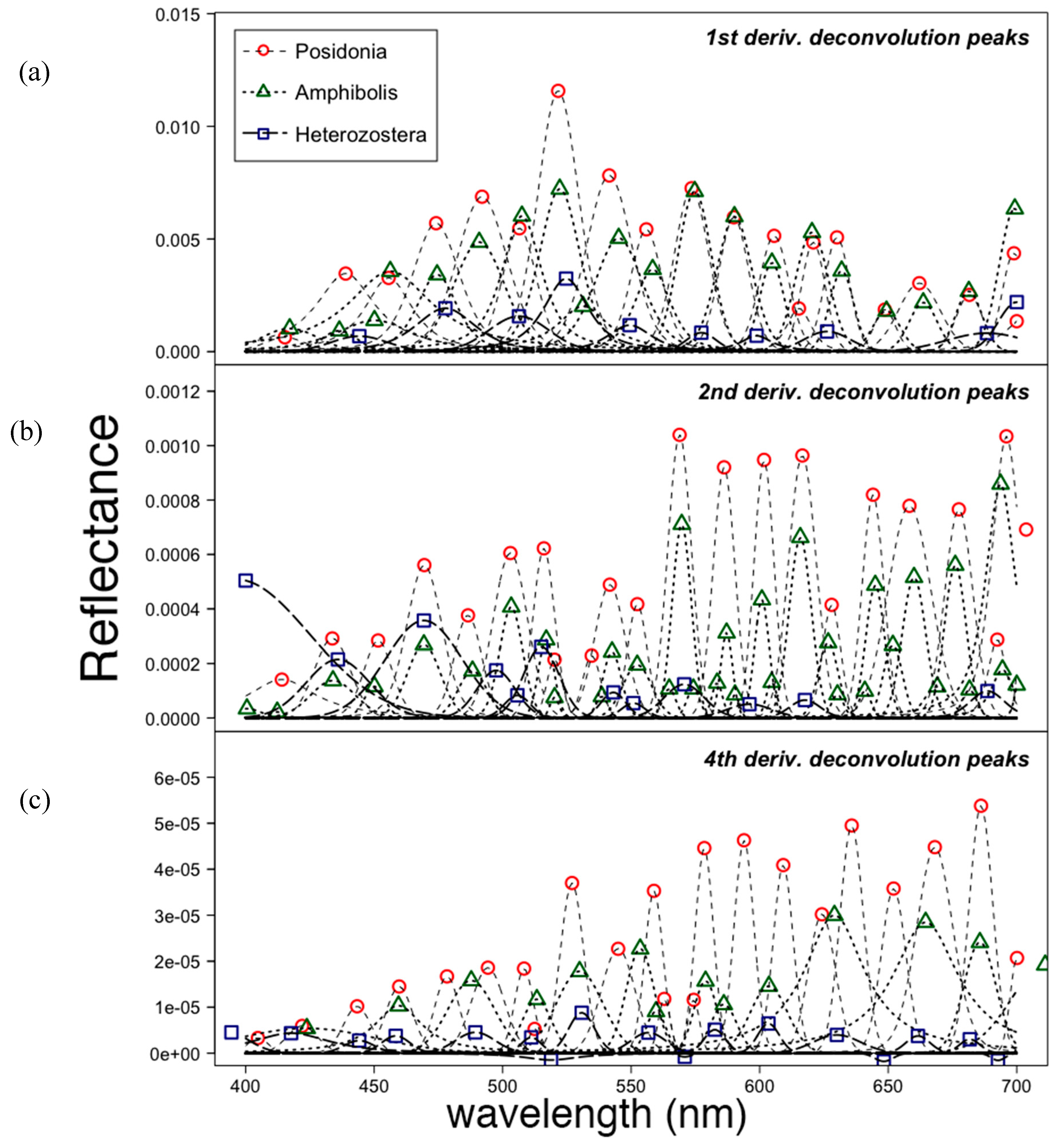
3.2. Spectral Deconvolution of Seagrass Spectra

In total, 201 peaks were used for the analyses of spectral profiles for the three seagrass genera. Their zero-order (original), first-order, second-order, and fourth-order derivatives produced 31, 50, 67, and 53, peaks, respectively (Figure 3, Figure 4a–c). Zero-order deconvolution derivative peaks had two instances at 583 and 708 nm where all three seagrasses produced overlapping peaks of differing reflectance amplitude heights (Figure 3 and Table S1). However, first-order derivatives have shown to help further highlight the subtle variations hidden within radiometric noise [25,37,46,47,48,49], and increase the accuracy of classification by up to a factor of 1.65, especially when compared to zero-order (original) reflectance spectra [37]. In this study, there were three specific instances (507, 575, and 700 nm) in which all three seagrasses each contained a characteristic first-order derivative peak at relatively the same 5-nm wavelength.
Moreover, first-derivative deconvolution analyses helped to reveal 11 distinct peaks within the visible spectrum (417, 456, 474, 491, 522, 590, 605, 621, 631, 649, and 681 nm) that were useful to differentiate Posidonia and Amphibolis (Figure 4a and Table S2). These analyses of first-derivatives further highlight differences between Posidonia and Amphibolis, with a Posidonia peak at 439 nm that has an order of magnitude higher reflectance than that of Amphibolis at 437 nm, as well as Posidonia spectral peaks at 542 and 556 nm with higher reflectance values than those of Amphibolis at 545 nm (Table S5). Additionally, first-order derivative peaks located at 455, 525, and 605 nm were used to separate and resolve Heterozostera from both Posidonia and Amphibolis.
Higher order derivatives have shown to help diminish the variations in illumination intensity [51,55] and have proven useful for distinguishing both seagrasses [48] as well as other benthic communities comprising of coral reefs [45]. In this study, second-order and fourth-order derivatives had higher frequency of specific bandwidths useful for discrimination of Heterozostera (Figure 4b,c; Tables S3 and S4). For example, second-order derivatives showed 12 peaks at 400, 435, 469, 497, 505, 515, 543, 551, 569, 596, 618, and 690 nm having higher frequency of spectral deconvolution peaks distinct for only Heterozostera (Figure 4b and Table S3). Similarly, deconvolution analyses of fourth-derivatives exhibited 17 peaks at 395, 420, 444, 459, 489, 511, 519, 530, 555, 571, 585, 603, 630, 650, 662, 682, and 693 nm, which are more frequently useful for discerning solely Heterozostera seagrass (Figure 4c and Table S4). However, the additional time and effort to perform calculations and run deconvolution analyses for higher order derivatives did not necessarily justify the improved species discrimination for all three seagrasses than compared to first-order derivatives. Therefore, the method of first-derivative deconvolution spectral peak analyses is evaluated as the most efficient derivative-based method for discriminating key, non-contiguous bandwidths throughout the visible light spectrum, reducing the number of dimensions necessary to be studied.
This is the first study that directly assessed the differences of original spectral profiles and compared their analyses to that of first-, second-, and fourth-order derivatives for distinguishing reflectance peaks of benthic bottom types. Deconvolution analyses proved to be a useful technique that provided novelty by reducing the number of wavelength dimensions within the visible light spectrum necessary to study and better understand submerged benthic reflectance profiles. Moreover, first-derivative spectral reflectance deconvolution analyses provided the most efficient method for discrimination of seagrass genera, revealing 11 distinct peaks relevant for providing a spectral signature. The use of hyperspectral data may be better suited for deconvolution analyses of these derivatives, especially since spectral signatures in heterogenous benthic environments obtained from multispectral imagery do not allow for such rigorous, detailed deconvolution of high spectral resolution [29,70]. The application of a detailed step-wise derivative assessment protocol that was developed in this study (outlined in Table S5) may be useful for discerning even minor differences within submerged vegetative bottom types, which may include algae and detritus. This is particularly useful for future studies involving vegetative indices [48] or remote sensing within optically shallow coastal waters.

3.3. Influence of Site Location

Site location had no significant effect on reflectance values throughout the visible light spectrum (p ≥ 0.05). This result is similar to other studies [5,14,55,71], suggesting that site-specific characteristics such as subtidal slope profile [64], wave energy [63], or mixing and dispersion [72] have no effect on spectral markers. In this study, proximity to a wastewater treatment plant (Bolivar site) or a sandy beach (Seacliff site) did not influence the spectral response. This bottom-up approach [73] for creating a spectral library can help prevent misclassification [23,55], including areas where distribution is sparse [26], such as in the Bolivar site [63]. The method reduces the number of dimensions to analyze, thereby allowing to solve for fundamental markers of submerged aquatic benthic types. The data can later be applied and integrated to solve higher-order operations, such as remote sensing algorithms that require a spectral library as part of a reference lookup table [22,73].

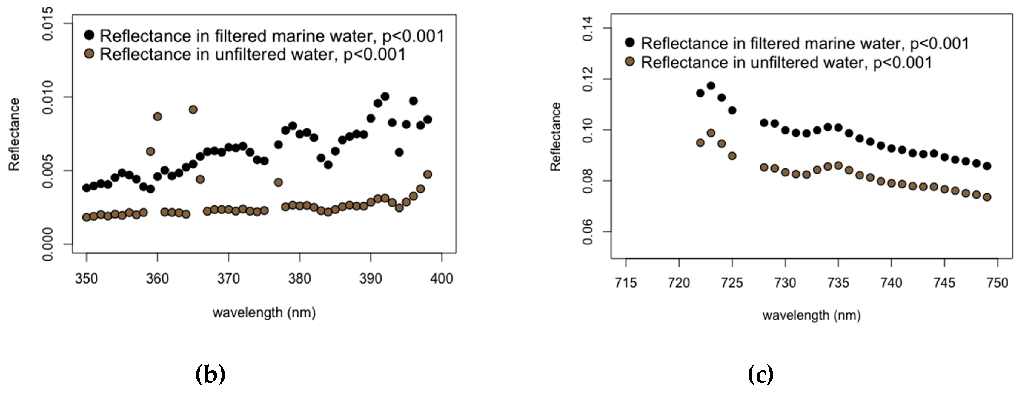
3.4. Effects of Marine Filtered Water

While spectral response of submerged vegetative benthic bottom types measured in filtered marine water had higher reflectance values (Figure 5), this significant effect (p ≤ 0.001) was confined to the tail ends of the visible light spectrum at 350–398 nm and 725–749 nm, respectively (Table S6). The higher reflectance values suggest that dissolved matter or very fine particles may be producing a dampening effect on the spectral responses, even though these effects are not statistically significant. This may include particles like phytoplankton, sediment, minerals, other suspended organic and inorganic matter, and dissolved organic substances which are commonly found within the water column [22,50,74]. Furthermore, application of results in this study showed that since detection of the submerged benthic bottom types focuses primarily on wavelengths within the visible light spectrum (380–750 nm) where light is able to penetrate the water column and reflect back to the sensor [5,24], the effects of measuring with filtered or unfiltered marine water will most likely not affect remote sensing of the submerged aquatic endmembers.

4. Conclusions

Results from this study reveal four major findings:
  • The bandwidth ratio of 566:689 helps distinguish seagrasses from sand, and the bandwidth ratio 566:600 may help distinguish seagrasses from algae and detritus.
  • Deconvolution analyses proved useful in the reduction of dimensions by identifying overlapping bandwidths of different seagrass genera and decreasing the number of wavelengths that need to be considered. Specifically, first-derivative deconvolution spectral peak analyses reveal to be the most efficient derivative-based method in isolating crucial, non-contiguous bandwidths throughout the visible light spectrum that can be used to distinguish seagrass genera.
  • Variations between local regions appear to have no effect on spectral endmembers, thereby making spectral reflectance values suitable markers for identifying submerged benthic bottom types throughout the world, not just within a particular region.
  • Fluctuations in marine water composition appear to have no significant effect on endmember selection for the detection of submerged aquatic vegetation.
From a systems analysis approach, integration of the findings in this study helped to produce a more robust spectral reflectance library that reduces dimensions by isolating key features and increases efficiency of data processing. Application of these findings involves using the library of endmember reflectance spectra developed in this study as effective hyperspectral remote sensing endmembers. In doing so, this in turn supports better and continued monitoring of changes in optically shallow coastal regions, particularly that of seagrass habitats. Thus, continued assessment of these detected changes contributes to the sustainability of seagrasses.

Supplementary Materials

The following are available online at https://www.mdpi.com/2071-1050/11/13/3695/s1. Table S1: List of characteristic spectral peak centers and amplitudes for (zero-order derivatives of) three seagrasses found within the coastal waters of metro-Adelaide, South Australia; Table S2: List of characteristic spectral peak centers and amplitudes for (first-order derivatives of) three seagrasses found within the coastal waters of metro-Adelaide, South Australia; Table S3: List of characteristic spectral peak centers and amplitudes for (second-order derivatives of) three seagrasses found within the coastal waters of metro-Adelaide, South Australia; Table S4: List of characteristic spectral peak centers and amplitudes for (fourth-order derivatives of) three seagrasses found within the coastal waters of metro-Adelaide, South Australia; Table S5: Five steps for differentiation of benthic bottom types found in South Australia study area; Table S6: Wavelengths at which reflectance of seagrass measured in filtered marine water (Whatman GF/C 1.2 μm glass microfiber filter, 90 mm diameter) were significantly higher than those in unfiltered marine water.

Author Contributions

C.-H.C., M.B., and M.F. suggested and supervised the conceptualization and idea of the research. C.-H.C. and T.K. conceived and designed the experiment; T.K. and C.H. troubleshooted, redesigned, and performed the experiments. C.H. processed and analyzed the acquired data. C.H. drafted the current paper; C.H., M.B., M.F., and T.K. edited the paper.

Funding

This research was funded in part by a research grant (Research Project No. CS7665) provided through the 2012–2013 Premier’s Research and Industry Fund (PRIF), a part of the Department of Further Education, Employment, Science, and Technology (DFEEST), Government of South Australia, Australia. C. Hwang was supported by funding from National Cheng Kung University (NCKU) Distinguished International Student Scholarship, NCKU Dept. of Engineering International Student Scholarship, NCKU Dept. of Engineering Research Assistantship, and CTCI Foundation Scholarship for Overseas Graduate Students.

Acknowledgments

The authors express their gratitude to G. Westphalen, A. Mussared, L. Van Der Linden, R. Daly, and the rest of the staff at Australian Water Quality Centre, SA Water, Adelaide, South Australia, Australia for assistance with fieldwork and data analyses.

Conflicts of Interest

The authors declare no conflict of interests.

References

  1. Hemminga, M.A.; Duarte, C.M. Seagrass Ecology; Cambridge University Press: Cambridge, UK, 2008; p. 312. [Google Scholar]
  2. Phinn, S.; Roelfsema, C.; Dekker, A.; Brando, V.; Anstee, J. Mapping seagrass species, cover and biomass in shallow waters: An assessment of satellite multi-spectral and airborne hyper-spectral imaging systems in Moreton Bay (Australia). Remote Sens. Environ. 2008, 112, 3413–3425. [Google Scholar] [CrossRef]
  3. Williams, S.L.; Heck, K.L., Jr. Seagrass Community Ecology. In Marine Community Ecology; Bertness, M.D., Gaines, S.D., Hay, M.E., Eds.; Sinauer Associates, Inc.: Sunderland, MA, USA, 2011; pp. 317–337. [Google Scholar]
  4. Duarte, C.M. The future of seagrass meadows. Environ. Conserv. 2002, 29, 192–206. [Google Scholar] [CrossRef] [Green Version]
  5. Fyfe, S.K. Spatial and temporal variation in spectral reflectance: Are seagrass species spectrally distinct? Limnol. Oceanogr. 2003, 48, 464–479. [Google Scholar] [CrossRef]
  6. Wabnitz, C.C.; Andréfouët, S.; Torres-Pulliza, D.; Müller-Karger, F.E.; Kramer, P.A. Regional-scale seagrass habitat mapping in the Wider Caribbean region using Landsat sensors: Applications to conservation and ecology. Remote Sens. Environ. 2008, 112, 3455–3467. [Google Scholar] [CrossRef]
  7. Borfecchia, F.; De Cecco, L.; Martini, S.; Ceriola, G.; Bollanos, S.; Vlachopoulos, G.; Belmonte, A.; Micheli, C. Posidonia oceanica genetic and biometry mapping through high-resolution satellite spectral vegetation indices and sea-truth calibration. Int. J. Remote Sens. 2013, 34, 4680–4701. [Google Scholar] [CrossRef]
  8. Cunha, A.H.; Assis, J.F.; Serrão, E.A. Reprint of Seagrasses in Portugal: A most endangered marine habitat. Aquat. Bot. 2014, 115, 3–13. [Google Scholar] [CrossRef]
  9. Ralph, P.J.; Durako, M.J.; Enríquez, S.; Collier, C.J.; Doblin, M.A. Impact of light limitation on seagrasses. J. Exp. Mar. Biol. Ecol. 2007, 350, 176–193. [Google Scholar] [CrossRef]
  10. Kimura, T.; Fujiwara, S.; Shibuno, T.; Mito, K.; Nakai, T.; Sasaki, Y.; Chang-Feng, D.; Gang, C. Status of Coral Reefs in East and North Asia (China, Hong Kong, Taiwan, South Korea and Japan). In Status of Coral Reefs of the World 2008; Wilkinson, C., Ed.; Global Coral Reef Monitoring Network and Reef and Rainforest Research Center: Townsville, Australia, 2008; pp. 145–158. [Google Scholar]
  11. Duarte, C.; Marba, N.; Santos, R. What May Cause Loss of Seagrasses? In European Seagrasses: An Introduction to Monitoring and Management; Borum, J., Duarte, C.M., Krause-Jensen, D., Greve, T.M., Eds.; EU Monitoring and Managing of European Seagrasses (M&MS) EVK3-CT-2000-00044: Brussels, Belgium, 2004; pp. 24–32. [Google Scholar]
  12. Waycott, M.; Duarte, C.M.; Carruthers, T.J.B.; Orth, R.J.; Dennison, W.C.; Olyarnik, S.; Calladine, A.; Fourqurean, J.W.; Heck, K.L., Jr.; Hughes, A.R.; et al. Accelerating loss of seagrasses across the globe threatens coastal ecosystems. Proc. Natl. Acad. Sci. USA 2009, 106, 12377–12381. [Google Scholar] [CrossRef] [Green Version]
  13. Barbier, E.B.; Hacker, S.D.; Kennedy, C.; Koch, E.W.; Stier, A.C.; Silliman, B.R. The value of estuarine and coastal ecosystem services. Ecol. Monogr. 2011, 81, 169–193. [Google Scholar] [CrossRef]
  14. Blackburn, D.T.; Dekker, A.G. Remote Sensing Study of Marine and Coastal Features and Interpretation of Changes in Relation to Natural and Anthropogenic Processes: Final Technical Report; ACWS Technical Report No. 6. Prepared for the Adelaide Coastal Waters Study Steering Committee; South Australian Environment Protection Authority (SA EPA): Adelaide, Australia, 2006.
  15. Nayar, S.; Collings, G.; Pfennig, P.; Royal, M. Managing nitrogen inputs into seagrass meadows near a coastal city: Flow-on from research to environmental improvement plans. Mar. Pollut. Bull. 2012, 64, 932–940. [Google Scholar] [CrossRef]
  16. Tanner, J.E.; Irving, A.D.; Fernandes, M.; Fotheringham, D.; McArdle, A.; Murray-Jones, S. Seagrass rehabilitation off metropolitan Adelaide: A case study of loss, action, failure and success. Ecol. Manag. Restor. 2014, 15, 168–179. [Google Scholar] [CrossRef]
  17. Hart, D. Seagrass Extent Change 2007–2013—Adelaide Coastal Waters; DEWNR Technical Note 2013/07; Government of South Australia. Department of Environment Water and Natural Resources: Adelaide, Australia, 2013; p. 19.
  18. Tanner, J.E.; Theil, M.; Fotheringham, D.G. Seagrass Condition Monitoring: Encounter Bay and Port Adelaide: Final Report Prepared for the Adelaide and Mount Lofty Ranges Natural Resources Management Board; SARDI Research Report, Series; Theil, M., Ed.; South Australian Research and Development Institution: West Beach, Australia, 2014; pp. 1324–2083.
  19. Clarke, K.; Hennessy, A.; Lewis, M. Adelaide Metropolitan Coastline benthic Habitat Mapping from Hyperspectral Imagery; Product A: Bare-substrate vs. non-bare Substrate; Prepared for SA Water, SA Department for Environment and Water, and SA Environmental Protection Authority; School of Biological Sciences, The University of Adelaide: Adelaide, Australia, 2018. [Google Scholar]
  20. Dekker, A.G.; Brando, V.E.; Anstee, J.M. Retrospective seagrass change detection in a shallow coastal tidal Australian lake. Remote Sens. Environ. 2005, 97, 415–433. [Google Scholar] [CrossRef]
  21. O’Neill, J.D.; Costa, M.; Sharma, T. Remote Sensing of Shallow Coastal Benthic Substrates: In situ Spectra and Mapping of Eelgrass (Zostera marina) in the Gulf Islands National Park Reserve of Canada. Remote Sens. 2011, 3, 975–1005. [Google Scholar] [CrossRef] [Green Version]
  22. Dekker, A.; Rando, V.; Anstee, J.; Fyfe, S.; Malthus, T.; Karpouzli, E. Remote Sensing of Seagrass Ecosystems: Use of Spaceborne and Airborne Sensors. In Seagrasses: Biology, Ecology and Conservation; Springer: Dordrecht, The Netherlands, 2006; pp. 347–359. [Google Scholar]
  23. Dunk, I.; Lewis, M. Seagrass and shallow water feature discrimination using HyMap imagery. In Proceedings of the 10th Australasian Remote Sensing Photogrammetry Conference, Adelaide, Australia, 21–25 August 2000. [Google Scholar]
  24. Brando, V.; Dekker, A.G. Satellite hyperspectral remote sensing for estimating estuarine and coastal water quality. IEEE Trans. Geosci. Remote Sens. 2003, 41, 1378–1387. [Google Scholar] [CrossRef]
  25. O’Neill, J.D.; Costa, M. Mapping eelgrass (Zostera marina) in the Gulf Islands National Park Reserve of Canada using high spatial resolution satellite and airborne imagery. Remote Sens. Environ. 2013, 133, 152–167. [Google Scholar] [CrossRef]
  26. Kakuta, S.; Takeuchi, W.; Prathep, A. Seaweed and seagrass mapping in Thailand measured by using Landsat 8 optical and texture properties. In Proceedings of the International Symposium on Remote Sensing (ISRS), Tainan, Taiwan, 22–24 April 2015. [Google Scholar]
  27. Medjahed, S.A.; Ouali, M. Band selection based on optimization approach for hyperspectral image classification. Egypt. J. Remote Sens. Space Sci. 2018, 21, 413–418. [Google Scholar] [CrossRef]
  28. Veys, C.; Hibbert, J.; Davis, P.; Grieve, B. An ultra-low-cost active multispectral crop diagnostics device. In Proceedings of the 2017 IEEE SENSORS, Glasgow, Scotland, 30 October–1 November 2017. [Google Scholar]
  29. Transon, J.; d’Andrimont, R.; Maugnard, A.; Defourny, P. Survey of Hyperspectral Earth Observation Applications from Space in the Sentinel-2 Context. Remote Sens. 2018, 10, 157. [Google Scholar] [CrossRef]
  30. Vahtmäe, E.; Kutser, T.; Martin, G.; Kotta, J. Feasibility of hyperspectral remote sensing for mapping benthic macroalgal cover in turbid coastal waters—A Baltic Sea case study. Remote Sens. Environ. 2006, 101, 342–351. [Google Scholar] [CrossRef]
  31. Chang, C.-H.; Liu, C.C.; Chung, H.W.; Lee, L.J.; Yang, W.C. Development and evaluation of a genetic algorithm-based ocean color inversion model for simultaneously retrieving optical properties and bottom types in coral reef regions. Appl. Opt. 2014, 53, 605–617. [Google Scholar] [CrossRef]
  32. Mumby, P.J.; Skirving, W.; Strong, A.E.; Hardy, J.T.; LeDrew, E.F.; Hochberg, E.J.; Stumpf, R.P.; David, L.T. Remote sensing of coral reefs and their physical environment. Mar. Pollut. Bull. 2004, 48, 219–228. [Google Scholar] [CrossRef]
  33. Patten, B.C. Systems approach to the concept of environment. Ohio J. Sci. 1978, 78, 206–222. [Google Scholar]
  34. Gallopin, G.C. Environmental and sustainability indicators and the concept of situational indicators. A systems approach. Environ. Model. Assess. 1996, 1, 101–117. [Google Scholar] [CrossRef]
  35. Hedley, J.D.; Mumby, P.J. A remote sensing method for resolving depth and subpixel composition of aquatic benthos. Limnol. Oceanogr. 2003, 48, 480–488. [Google Scholar] [CrossRef] [Green Version]
  36. Hornberger, G.M.; Spear, R.C. Approach to the preliminary analysis of environmental systems. J. Environ. Mgmt. 1981, 12, 7–18. [Google Scholar]
  37. Karpouzli, E.; Malthus, T.J.; Place, C.J. Hyperspectral discrimination of coral reef benthic communities in the western Caribbean. Coral Reefs 2004, 23, 141–151. [Google Scholar] [CrossRef]
  38. Miglani, A. Hyperspectral Remote Sensing—An Overview. 7 December 2010. Available online: https://www.geospatialworld.net/article/hyperspectral-remote-sensing-an-overview/ (accessed on 13 April 2019).
  39. Takebe, M.; Yoneyama, T.; Inada, K.; Murakami, T. Spectral reflectance ratio of rice canopy for estimating crop nitrogen status. Plant Soil 1990, 122, 295–297. [Google Scholar] [CrossRef]
  40. Christensen, S.; Goudriaan, J. Deriving light interception and biomass from spectral reflectance ratio. Remote Sens. Environ. 1993, 43, 87–95. [Google Scholar] [CrossRef]
  41. Gitelson, A.A.; Merzlyak, M.N.; Lichtenthaler, H.K. Detection of red edge position and chlorophyll content by reflectance measurements near 700 nm. J. Plant Physiol. 1996, 148, 501–508. [Google Scholar] [CrossRef]
  42. Han, L.; Rundquist, D.C. Comparison of NIR/RED ratio and first derivative of reflectance in estimating algal-chlorophyll concentration: A case study in a turbid reservoir. Remote Sens. Environ. 1997, 62, 253–261. [Google Scholar] [CrossRef]
  43. Demetriades-Shah, T.H.; Steven, M.D.; Clark, J.A. High resolution derivative spectra in remote sensing. Remote Sens. Environ. 1990, 33, 55–64. [Google Scholar] [CrossRef]
  44. Scheinost, A.; Chavernas, A.; Barrón, V.; Torrent, J. Use and limitations of second-derivative diffuse reflectance spectroscopy in the visible to near-infrared range to identify and quantify Fe oxide minerals in soils. Clays Clay Miner. 1998, 46, 528–536. [Google Scholar] [CrossRef]
  45. Hochberg, E.J.; Atkinson, M.J. Spectral discrimination of coral reef benthic communities. Coral Reefs 2000, 19, 164–171. [Google Scholar] [CrossRef]
  46. Han, L. Spectral reflectance of Thalassia testudinum with varying depths. In Proceedings of the IEEE International Geoscience and Remote Sensing Symposium, Toronto, ON, Canada, 24–28 June 2002; pp. 2123–2125. [Google Scholar]
  47. Bargain, A.; Robin, M.; Le Men, E.; Huete, A.; Barillé, L. Spectral response of the seagrass Zostera noltii with different sediment backgrounds. Aquat. Bot. 2012, 98, 45–56. [Google Scholar] [CrossRef]
  48. Bargain, A.; Robin, M.; Méléder, V.; Rosa, P.; Le Menn, E.; Harin, N.; Barillé, L. Seasonal spectral variation of Zostera noltii and its influence on pigment-based Vegetation Indices. J. Exp. Mar. Biol. Ecol. 2013, 446, 86–94. [Google Scholar] [CrossRef]
  49. Fulton, S. An Analysis of the Spectral Reflectance Separability of Amphibolis Griffithii and Posidonia Sinuosa at Different Water Depths, in School of the Environment; The Flinders University of South Australia: Adelaide, Australia, 2014; p. 97. [Google Scholar]
  50. Dierssen, H.M.; Kudela, R.M.; Ryan, J.P.; Zimmerman, R.C. Red and black tides: Quantitative analysis of water-leaving radiance and perceived color for phytoplankton, colored dissolved organic matter, and suspended sediments. Limnol. Oceanogr. 2006, 51, 2646–2659. [Google Scholar] [CrossRef] [Green Version]
  51. Tsai, F.; Philpot, W. Derivative analysis of hyperspectral data. Remote Sens. Environ. 1998, 66, 41–51. [Google Scholar] [CrossRef]
  52. Treilibs, C.; Lewis, M.; Sparrow, B. Seagrass Discrimination and Mapping in Association with Atlantic Salmon Aquaculture, Cape Jaffa, South Australia: Report to the Native Vegetation Council; The University of Adelaide: Adelaide, Australia, 2005; p. 40. [Google Scholar]
  53. Poulsen, J.; French, A. Discriminant Function Analysis (DA); San Francisco State University: San Francisco, CA, USA, 2001. [Google Scholar]
  54. Maritorena, S.; Morel, A.; Gentili, B. Diffuse reflectance of oceanic shallow waters: Influence of water depth and bottom albedo. Limnol. Oceanogr. 1994, 39, 1689–1703. [Google Scholar] [CrossRef]
  55. Holden, H.; LeDrew, E. Hyperspectral identification of coral reef features. Int. J. Remote Sens. 1999, 20, 2545–2563. [Google Scholar] [CrossRef]
  56. Davies, T. The new automated mass spectrometry deconvolution and identification system (AMDIS). Spectrosc. Eur. 1998, 10, 24–27. [Google Scholar]
  57. Zhang, Q.; Alfarra, M.R.; Worsnop, D.R.; Allan, J.D.; Coe, H.; Canagaratna, M.R.; Jimenez, J.L. Deconvolution and quantification of hydrocarbon-like and oxygenated organic aerosols based on aerosol mass spectrometry. Environ. Sci. Technol. 2005, 39, 4938–4952. [Google Scholar] [CrossRef]
  58. Hasler-Sheetal, H.; Fragner, L.; Holmer, M.; Weckwerth, W. Diurnal effects of anoxia on the metabolome of the seagrass Zostera marina. Metabolomics 2015, 11, 1208–1218. [Google Scholar] [CrossRef] [Green Version]
  59. Bryars, S.; Collings, G.; Nayar, S.; Westphalen, G.; Miller, D.; O’Loughlin, E.; Fernandes, M.; Mount, G.; Tanner, J.; Wear, R.; et al. Assessment of the Effects of Inputs to the Adelaide Coastal Waters on the Meadow Forming Seagrasses, Amphibolis and Posidonia; Task EP 1 Final Technical Report; ACWS Technical Report No. 15. Prepared for the Adelaide Coastal Waters Study Steering Committee (Publication No. RD01/0208-19); South Australian Research and Development Institute (Aquatic Sciences): Adelaide, Australia, 2006.
  60. Bryars, S.; Rowling, K. Benthic habitats of eastern Gulf St Vincent: Major changes in benthic cover and composition following European settlement of Adelaide. Trans. R. Soc. S. Aust. 2009, 133, 318–338. [Google Scholar]
  61. Westphalen, G.; Collings, G.; Wear, R.; Fernandes, M.; Bryars, S.; Cheshire, A. A review of Seagrass Loss on the Adelaide Metropolitan Coastline; ACWS Technical Report No. 2. Prepared for the Adelaide Coastal Waters Study Steering Committee (Publication No. RD04/0073); South Australian Research and Development Institute (Aquatic Sciences): Adelaide, Australia, 2005.
  62. Bryars, S.; Miller, D.; Collings, G.; Fernandes, M.; Mount, G.; Wear, R. Field Surveys 2003–2005: Assessment of the Quality of Adelaide’s Coastal Waters, Sediments and Seagrasses; ACWS Technical Report No. 14. Prepared for the Adelaide Coastal Waters Study Steering Committee. Publication No. RD01/0208-15; South Australian Research and Development Institute (Aquatic Sciences): Adelaide, Australia, 2006.
  63. Bryars, S.; Rowling, K. Chapter 1. Benthic habitats of eastern Gulf St Vincent: Major changes in seagrass distribution and composition since European settlement of Adelaide. In Restoration of Coastal Seagrass Ecosystems: Amphibolis Antarctica in Gulf St Vincent, South Australia; Bryars, S., Ed.; SARDI Aquatic Sciences Publication No. F2008/000078, SARDI Research Report Series No. 277; South Australian Research and Development Institute (Aquatic Sciences): Adelaide, Australia, 2008; pp. 5–27. [Google Scholar]
  64. Bone, Y.; Deer, L.; Edwards, S.A.; Campbell, E. Adelaide Coastal Waters Study Coastal Sediment Budget; ACWS Technical Report No. 16 prepared for the Adelaide Coastal Waters Study Steering Committee; Adelaide University, Department of Geology: Adelaide, Australia, 2006. [Google Scholar]
  65. Joyce, K.E.; Phinn, S.R. Bi-directional reflectance of corals. Int. J. Remote Sens. 2002, 23, 389–394. [Google Scholar] [CrossRef]
  66. Ocean Optics. OceanView Installation and Operation Manual; Document Number 000-20000-310-02-201503; Ocean Optics: Winter Park, FL, USA, 2013. [Google Scholar]
  67. Ocean Optics. JAZ Installation and Operation Manual; Document Number 013-RD000-000-02-201502; Ocean Optics: Winter Park, FL, USA, 2010. [Google Scholar]
  68. Savitzky, A.; Golay, M.J.E. Smoothing and Differentiation of Data by Simplified Least Squares Procedures. Anal. Chem. 1964, 36, 1627–1639. [Google Scholar] [CrossRef]
  69. Han, L.; Rundquist, D.C. The spectral responses of Ceratophyllum demersum at varying depths in an experimental tank. Int. J. Remote Sens. 2003, 24, 859–864. [Google Scholar] [CrossRef]
  70. Barillé, L.; Robin, M.; Harin, N.; Bargain, A.; Launeau, P. Increase in seagrass distribution at Bourgneuf Bay (France) detected by spatial remote sensing. Aquat. Bot. 2010, 92, 185–194. [Google Scholar] [CrossRef]
  71. Dekker, A.; Phinn, S.R.; Anstee, J.; Bissett, P.; Brando, V.E.; Casey, B.; Fearns, P.; Hedley, J.; Klonowski, W.; Lee, Z.P.; et al. Intercomparison of shallow water bathymetry, hydro-optics, and benthos mapping techniques in Australian and Caribbean coastal environments. Limnol. Oceanogr. Methods 2011, 9, 396–425. [Google Scholar] [CrossRef] [Green Version]
  72. Wilkinson, J.; Pearce, M.; Cromar, N.; Fallowfield, H. Audit of the Quality and Quantity of Treated Wastewater Discharging from Wastewater Treatment Plants (WWTPs) to the Marine Environment; ACWS Technical Report No. 1. Prepared for the Adelaide Coastal Waters Study Steering Committee; Flinders University of South Australia, Department of Environmental Health: Adelaide, Australia, 2003. [Google Scholar]
  73. Hochberg, E.J.; Atkinson, M.J.; Andréfouët, S. Spectral reflectance of coral reef bottom-types worldwide and implications for coral reef remote sensing. Remote Sens. Environ. 2003, 85, 159–173. [Google Scholar] [CrossRef]
  74. Greve, T.M.; Binzer, T. Which Factors Regulate Seagrass Growth and Distribution? In European Seagrasses: An Introduction to Monitoring and Management; Borum, J., Borum, J., Duarte, C.M., Krause-Jensen, D., Greve, T.M., Eds.; EU Monitoring and Managing of European Seagrasses (M&MS) EVK3-CT-2000-00044: Brussels, Belgium, 2004; pp. 19–23. [Google Scholar]
Figure 1. Map of sampling sites located around both Bolivar and Seacliff Sites. These sites are north and south of metropolitan Adelaide in Gulf St. Vincent, South Australia, respectively.
Sustainability 11 03695 g001
Figure 2. Spectral reflectance profiles of dominant benthic bottom types in study area with 75th percentile (Q3), mean (average), and 25th percentile (Q1) showing variation of measurements for each wavelength.
Sustainability 11 03695 g002
Figure 3. Zero derivative (raw spectral) deconvolution peak analyses of dominant seagrass bottom types in the study area.
Sustainability 11 03695 g003
Figure 4. (a) First derivative, (b) second derivative and (c) fourth derivative deconvolution peak analyses of dominant seagrass bottom types in the study area.
Sustainability 11 03695 g004
Figure 5. (a) Reflectance of seagrasses measured in filtered marine water and unfiltered marine water. Note that “NS” refers to p-values being not significant. (b,c) Insets of statistically significant reflectance values of seagrasses from 350–400 nm, and from 720–750 nm, respectively.
Sustainability 11 03695 g005aSustainability 11 03695 g005b
Table 1. Bandwidth ratios useful for differentiating among benthic bottom types.
Slope Ratio at
Bottom Type λ =   (566:600) λ =   (566:689)
Posidonia1.384.52
Amphibolis1.033.77
Heterozostera1.294.93
Sand0.770.54

