Article

Data Science Solutions for Retail Strategy to Reduce Waste Keeping High Profit

by
Gen Sakoda
1,†,
Hideki Takayasu
2,3,† and
Misako Takayasu
1,3,*,†
1
Department of Mathematical and Computing Sciences, School of Computing, Tokyo Institute of Technology, 4259 Nagatsuta-cho, Midori-ku, Yokohama 226-8502, Japan
2
Sony Computer Science Laboratories, 3-14-13 Higashi-Gotanda, Shinagawa-ku, Tokyo 141-0022, Japan
3
Institute of Innovative Research, Tokyo Institute of Technology, 4259 Nagatsuta-cho, Midori-ku, Yokohama 226-8502, Japan
*
Author to whom correspondence should be addressed.
These authors contributed equally to this work.
Sustainability 2019, 11(13), 3589; https://doi.org/10.3390/su11133589
Submission received: 29 May 2019 / Revised: 24 June 2019 / Accepted: 25 June 2019 / Published: 29 June 2019
(This article belongs to the Section Economic and Business Aspects of Sustainability)

Abstract

:
Waste reduction in retail is a fundamental problem for sustainability. Among waste reduction approaches such as recycling and donation, stock management based on demand estimation which leads to mitigate waste generation and maintain a high profit is expected to play an important role. However, demand estimation is generally difficult because fluctuations in sales are quite volatile, and stock-out leads to incomplete demand observation. Here, we propose data science solutions to estimate non-stationary demand with censored sales data including stock-outs and realize scientific stock management. Concretely, we extend a non-stationary time series analysis method based on Particle Filter to handle censored data, and combine it with the newsvendor problem formula to determine the optimal stock. Moreover, we provide a way of pricing waste reduction costs. A method to verify consistency between the statistical model and sales data is also proposed. Numerical analysis using actual Point-Of-Sales data in convenience stores shows food waste could be reduced several tenths percent keeping high profits in most cases. Specifically, in cases of foods disposed of frequently about 75% of working days, food waste decreases to about a quarter with the profit increases by about 140%. The way of pricing waste reduction costs tells new insights such as 27% waste reduction is achieved by 1% profit loss. Our method provides a practical solution for food waste reduction in the retail sector.

1. Introduction

1.1. Background

The United Nations predicts the world population reaches 8.6 billion in 2030 and 9.8 billion in 2050 [1]. Establishment of sustainable food systems for increasing food demand is essential. In this context, reduction of food loss and waste draws special attention since the one-third of foods are lost or wasted every year, which amounts to four times as much food required yearly for eliminating global hunger [2]. While food losses predominantly occur due to inefficient harvesting, storage facilities, infrastructural conditions and access to the market in low- and middle-income countries [3], food waste depends on such factors as cultural habits, meal planning, and shopping behavior [4]. The wasteful practices of the food industry and consumers in high-income countries are the predominant drivers for food waste [5].
Food waste reduction at retail is listed in the Sustainable Development Goals (SDGs) Target 12.3 [6]. In this study, we forcus on food waste reduction in the retail sector. We possess detailed sales data of a convenience store which contains records of disposal in addition to sales. Utilizing this data, we can consider specific measures for retail from the viewpoint of data science.

1.2. Literature Review on Food Waste Reduction

Component ratio analyses of total food waste [7,8,9] indicate that the household is the largest producer of food waste (53–71%), followed by food manufacturing and processing companies (17–30%), food service providers (9–12%) and retail (2–9%). Though the percentage of retail is relatively small, comprehensive initiatives including in retail are essential as the SDGs Target 12.3 covers the waste reduction in the retail sector. Studies on food waste constituent ratio in retail show it mainly consists of perishables, particularly, either bread or fruit and vegetables [10,11]. Concretely, a recent study shows that 30% originates from bread and 29% from fruit and vegetables in the total wasted mass [12]. Another recent research discussed the economic cost and the climate impact in addition to the mass of fruit and vegetable waste, and specified hotspot categories in Swedish food retail market [13].
Many strategies for food waste reduction have been proposed. For example, the concept of food recovery and food redistribution, specifically, food sharing including donating and bartering initiatives, have been widely spread in developed countries [14,15]. Recently, startups offer online platforms which help exchange surplus food [16,17] and cook and eat together [18,19]. Food waste valorization [20,21] is another primary strategy that converts food waste into chemicals, materials, and energy, or extracts high-value target compound from food waste. Specifically, techniques such as thermochemical, biochemical, fermentation, and extraction processes are used to obtain biofuels, drug, cosmetics, animal feed, fertilizer supply, compositing from food waste. Increasing demand for chemicals, materials, and fuels for sustainable future makes food waste valorization important approach. Customer awareness campaigns such as “Love Food Hate Waste” scheme introduced by WRAP in 2007 [22] and “I Value Food” project organized by Sustainable America [23], are also held for customer’s voluntary food waste reduction.
Actual practices taken for waste reduction at grocery retail stores in the United Kingdom has been studied recently [24]. Food donation to charities and food banks is conducted with making use of partnerships with surplus food distribution platforms such as FareShare [25] and local charities on food donations. Software and online platforms like “Food Cloud” [26] simplify the donating process, which helps retail managers grasp foods approaching their expiration date and communicate with registered charities. Other approaches include changing the labeling on products which shows just packaging date instead of “best before date” [27,28], investment in packaging and storage to improve food quality and shelf life, and price reduction for food items which do not meet company’s aesthetical standards or are approaching expiration date. Customer awareness campaigns, surplus foods for staff canteen, bakery waste sent for animal feeding, cooking oils diverted for biofuel production are also reported.
It is pointed out that waste management program which ignores social aspects of management and professional skills is prone to failure [29]. There exists a study identifying innovative food waste management practices and evaluating food service manager’s perspectives on these innovations [30]. In their study, incremental strategies in operational process and developments in current technology rather than radical innovations are reported to be dominant in the restaurants in Switzerland. Constraints to adoption of innovations are ranging from internal factors (lack of space, infrastructure, etc.), human capital factors (lack of time or staff, motivations, skills, etc.), external factors(uncollaborative customers, suppliers, etc.) and legal factors(local legislation, etc.). The primary driver for the adoption of food mitigation practices is financial savings and reputational gains [24,30]. Another research also reveals complex relationships in many drivers, namely, policy, private initiatives, consumer behavior, food waste impact, and food industry issues, and examine the effect of changing policies [31]. Technical proposal for waste reduction needs to take these managerial views into account for practical implementation.

1.3. Literature Review on Stock Management and Demand Estimataion

We explore specific solutions for food waste reduction in retail using the sales data. Scientific stock management based on precise demand estimation with sales data is a candidate for waste prevention. Related researches have been widely conducted. The newsvendor problem is a representative example. Perishable products such as newspapers and foods are disposed of when remaining unsold at the end of the day, while stock-out of those result in opportunity loss. The newsvendor problem tells the optimal stock to maximize profit under the fluctuating demand. There exist a wide variety of extension [32,33,34]. For demand uncertainty, Bayesian approach, specifically Bayesian Dynamic Programming (BDP), is proposed to update the uncertain demand distribution with sales data [35,36,37]. After the adverse effect of stock-outs in sales data on demand estimation is shown [38,39], BDP for censored sales data because of stock-outs is proposed [40,41]. Since BDP with censored data is tractable only when demand distribution is assumed to be exponential and Weibull distribution, more general demand distribution such as Poisson distribution cannot be assumed. Instead of solving BDP rigorously, heuristics such as the myopic policy which optimize the stock without considering future demand, are also developed [42,43]. Though the myopic policy is proved to order more than the optimal stock [44,45], it is shown that the difference between the myopic and the optimal stock is generally bellow 1% in most cases [46]. While BDP needs to assume the functional form of the demand distribution, some non-parametric approaches are also proposed [47,48,49,50]. Although vast researches have been conducted, these BDP and non-parametric approaches for censored demand assume the time dependency of the demand is stationary [51].
For non-stationary demand, there exist a variety of studies. For example, Markov Modulated Demand Process (MMD) provides non-stationary demand estimation [52,53,54,55]. BDP for sales time series with a single change point is also studied [56]. For non-stationary demand with auto-correlation, Auto Regressive Integrated Moving Average (ARIMA) is adapted [57,58,59,60]. Machine learning approaches for sales time series with underlying patterns is also studied [61,62,63]. However, these non-stationary demand analyses are not ready to handle censored sales data.
As for the conventional studies on waste reduction using sales data, there exists research on quantifying the amount of waste reduction, that reveals the amount of packaging waste of the shampoo and hair conditioner is reduced by introducing refill packages [64]. Other researches using food sales data, such as milk [65], bread [66,67], foods in convenience stores [68,69] and grocery retailing [70], mainly aim at estimating demand and a way for waste reduction is not proposed.

1.4. The Aim and Contribution to the Literature

Our aim and contribution are to provide a practical solution for demand estimation and stock management under non-stationary and censored demand, which realizes food waste reduction keeping high profit. We recently proposed a non-stationary time series analysis method [71] which is suitable for sales data analysis since it incorporates a recently discovered nature of the fluctuation of the sales data, namely, Taylor’s law [72]. Specifically, the sales process is basically the Poisson process of which fluctuation width is known to be the square root of the mean, however, the fluctuation width is proportional to the mean when the mean is large, which is caused by the effect of fluctuation in the population (customer) [73]. Our study [71] shows that the parameter (demand) estimation of non-stationary sales data without considering Taylor’s law leads to a misreading of the abnormal fluctuation in sales data as non-stationary changes of the demand, that results in poor accuracy of demand estimation.
In this study, we extend this non-stationary time series analysis method to be applicable to the demand estimation with censored sales data. We combine this method with the newsvendor problem formula to determine the optimal stock for each time. Moreover, we extend the newsvendor problem formula to determine the stock realizing the desired waste reduction, with pricing the cost of the waste reduction. We verify the effectiveness of our method for food waste reduction keeping high profit with the actual sales and disposal data.

2. Methods

Our method is based on the two methods, namely, the newsvendor problem [32,33,34] and the parameter estimation method for non-stationary time series [71]. In this section, we review these methods briefly and explain the detail of our method.

2.1. Newsvendor Problem

In the retail sector, managing the stock of perishable items such as newspaper and daily food is a challenging task, since those remaining unsold at the end of the day are to be disposed of, while sold-out of those results in opportunity loss. The difficulty in determining the optimal stock lies in the fluctuation of the demand. Namely, the demand k is not supposed to be constant but follow some Probability Density Function (PDF) m ( k ) . The newsvendor problem tells us how much stock s should we prepare a day for the fluctuating demand m ( k ) to obtain the maximum profit. Assuming the cost c and price p, the expected profit R ( s ) is written as follows:
R ( s ) = p { k = 0 s k m ( k ) + k = s + 1 s m ( k ) } c s
Here, we assume the stock s is discrete and the unsold products at the end of the day are disposed of. The stock s * for the maximum profit is obtained by calculating the differential value of the Equation (1).
R ( s + 1 ) R ( s ) = p k = s + 1 m ( k ) c = 0
Thus, s * is written with the Inverse of Cumulative Distribution Function(CDF) M 1 ( k ) , where M ( k ) = P r o b ( K > k ) ,44]
s * = M 1 ( c p )
Equation (3) means the stock s * for the maximum profit can be calculated with the cost ratio c / p , and the demand distribution m ( k ) which determines M 1 ( k ) .

2.2. Assumption of the Demand Distribution

To solve the Equation (3), the functional form of the demand distribution needs to be assumed. In conventional researches, distributions such as the Poisson distribution [38], the Normal distribution [39], and the negative binomial distribution [74] are assumed. Meanwhile, our recent study [73] on sales data of a convenience store reveals it follows Taylor’s law [72]. That is, underlying fluctuation in the population of the observing objects (customers) affects the fluctuation of the observation of the Poisson process. Sales is basically a Poisson process of which fluctuation is known to be the square root of the mean value λ , but the fluctuation of the number of the customer leads to the fluctuation of the demand following the demand mean value λ linearly, when the demand mean is large. The standard deviation σ of Taylor’s fluctuation scaling is generally written as follows:
σ = λ + ( γ · λ ) 2
where γ is the proportionality constant of Taylor’s fluctuation scaling. We incorporate this knowledge into the assumption of the demand distribution m ( k | λ ) for given demand mean value λ . Namely, we adopt the Poisson distribution P o ( λ ) for small λ , otherwise the Normal distribution N ( λ , σ ) with the fluctuation σ corresponding to the Equation (4).
m ( k | λ ) = P o ( λ ) , if λ < 20 N ( λ , λ + ( γ · λ ) 2 ) , otherwise
Here, we approximate the Poisson distribution to the Normal distribution for λ 20 . Although the approximation can be performed for λ 10 , [75] we adopt λ 20 since the skewness of the Poisson distribution of λ = 20 is 30 % smaller than that of λ = 10 , therefore, closer to 0, that is the value of skewness of the normal distribution, whereas the change ratio of the standard deviation by Taylor’s fluctuation scaling at λ < 20 is below 10 % , where γ = 0.1 . The specific γ value for the sales time series used in this research is 0.12 [73].
The Equations (3) and (5) allow calculating the optimal stock s * for a demand mean value λ for each cost ratio. For example, assuming λ = 10 , the M 1 ( k ) in the Equation (3) is calculated using the Poisson distribution with λ = 10 . The optimal stocks s * for the cost ratio 0.9, 0.7, 0.5 are determined to be 6, 8, 10, respectively. Assuming λ = 50 and the proportionality constant of Taylor’s fluctuation scaling γ = 0.1 , the Normal distribution in the Equation (5) is used to determine the optimal stock s * . In this case, the optimal stock s * for the cost ratio 0.9, 0.7, 0.5 are determined to be 39, 45, 50, respectively. The optimal stock depends on the cost ratio and the demand distribution in this way. The detailed information is provided in the Appendix A (Figure A8).

2.3. Parameter Estimation of the Demand Distribution

To determine m ( k | λ ) in the Equation (5), we need to estimate the demand parameter λ for each time t. We have to consider that the demand is generally non-stationary and the fluctuation of the sales data follows Taylor’s law. We recently proposed parameter estimation method for non-stationary time series with Taylor’s fluctuation scaling [71].
In this method, the State Space Model (SSM) [76] is adopted for statistical modeling of sales data. The SSM assumes an observation data y t at time t is obtained stochastically by underlying invisible state x t , and x t is also stochastically determined by x t 1 . Non-stationarity of a time series is modeled by a transition function of x t 1 to x t , which is called the system model. The system model we proposed for tracking non-stationary parameter is as follows:
x t = δ ( x t 1 + ν t )
δ ( x ) = x , if x > 0 0 , otherwise
ν t ( 1 m ) · N ( 0 , α · x t 1 ) + m · U ( β , β )
where ν t in the Equation (8) is a stochastic variable which governs the transition from x t 1 to x t in the Equation (6). The value of x t is limited to be non-negative by the delta function in the Equation (7) since the Poisson parameter λ (or x t ) needs to be positive. The tilde (∼) in the Equation (8) denotes that ν t follows the distribution in the right side of the formula, namely, the superposition of Normal distribution N ( 0 , α · x t 1 ) with the mean value zero and the standard deviation α · x t 1 ( 0 < α ), and Uniform distribution U ( β , β ) which takes values between β and β ( 0 < β ). m characterizes the ratio of superposition of the Normal and the Uniform distribution ( 0 m 1 ). The superposition of two distributions considers the case where x t generally follows the Normal distribution, but occasionally changes up to β with a small probability m. The value of β is determined so that the range of the Uniform distribution is much larger than the fluctuation of the Normal distribution ( α · x t 1 ), that allows a large change of x t . m, α , β are hyper parameters. In this research, we adopted m = 0.05 , α = 0.005 and β = 4 x t 1 by examining Root Mean Squared Error of λ estimation of some artificial time series. The detailed information of the determination of the hyper parameters is provided in the Appendix of the reference [71].
We specify the observation model in the SSM, which describes the observation of data y t from the state x t as follows:
y t P o ( x t ) , if λ < 20 N ( x t , x t + ( γ · x t ) 2 ) , otherwise
Here, Taylor’s fluctuation scaling at large x t is considered as in the Equation (5). Wide fluctuation caused by Taylor’s fluctuation scaling is correctly treated as fluctuation, instead of a non-stationary change of x t , by this term.
This SSM can be solved with the Particle Filter [77,78] to determine the state x t at time t. The Particle Filter is a kind of Monte Carlo simulation which approximates an arbitrary PDF of the state x t as the distribution of Monte Carlo sample values, which is called the particle distribution. The particle distribution is updated with the observation data y t at time t in accordance with the likelihood of each particle value.
The likelihood function for our observation model is PDF of the Poisson and Normal distribution in the Equation (9). We extend our model for the case of a censored observation. We adopt the following likelihood function F ( k t | θ ) for a censored observation k t [79] for updating the particle distribution.
F ( k t | θ ) = s t f ( k | θ ) d k
Thus, the likelihood function for our SSM is described as follows:
p ( y t | x t ) = 1 2 π σ t 2 exp ( ( y t x t ) 2 2 σ t 2 ) , if x t 20 and non-censored 1 2 π σ t 2 m = y t exp ( ( m x t ) 2 2 σ t 2 ) else if x t 20 and censored x t y t · exp ( x t ) y t ! , else if x t < 20 and non-censored m = y t x t m · exp ( x t ) m ! , otherwise
where σ t = x t + ( γ · x t ) 2 .
The number of Monte Carlo samples is set to N = 10,000 and the initial particles are generated by the Equations (6)–(8) assuming x 0 = y 1 , namely sales k 1 for simplicity. In the case k 1 = 0 , the initial particles are generated assuming x 0 = 1 . The λ value for each time t is obtained with calculating the median, instead of the mean, of the Monte Carlo samples of x t since its robustness against variations of particle values. While the SSM can be solved with Markov Chain Monte Carlo (MCMC) [80], the Particle Filter is selected since it can stably solve the SSM even with a small amount of data.

2.4. Pricing the Cost of Waste Reduction

We formulate the expected disposal amount d t * as the following equation.
d t * = k = 0 s t * 1 ( s t * k ) m ( k | λ t )
where s t * is the stock for the maximum profit at time t which is determined with the Equation (3), and m ( k | λ t ) is the demand distribution shown in the Equation (5). Thus, the stock s ( α ) t for reducing disposal α ( 0 α 1 ) times compared to d t * is expressed as follows:
s ( α ) t = arg min 0 s s * ( | α d t * k = 0 s 1 ( s k ) m ( k | λ t ) | )
The profit R ( s ( α ) t ) is estimated as follows:
R ( s ( α ) t ) = p ( s ( α ) t α d t * ) c s ( α ) t
Thus, we can estimate the cost of the waste reduction by examining R ( s ( α ) t ) / R ( s t * ) .

2.5. Stock Determination for Fine Control of Waste Reduction

The demand distribution m ( k | λ t ) in the Equation (13) is assumed to be the Poisson distribution at small λ as shown in the Equation (5). Since the Poisson distribution is discrete, the stock s ( α ) t obtained with the Equation (13) is inevitably discrete, that leads to poor controllability of the waste reduction. For example, assuming the demand mean λ = 10 and the target disposal ratio 0.5 α 1.0 , the stock value s ( α ) t can only be two values, namely, 7 or 8. We modify the Poisson distribution with the Γ function to handle a real number stock value as follows:
m ( k | λ ) = λ k · exp ( λ ) Γ ( k + 1 ) , if λ < 20 N ( λ , λ + ( γ · λ ) 2 ) , otherwise
There is one more thing to consider for fine control of waste reduction. The actual stock values for products in the retail, such as riceballs and meat buns, need to be discrete. We propose a probabilistic selection of the two stock value around s ( α ) t to approximate the real number of s ( α ) t under many trials. For example, if the target stock s ( α ) t is 10.3 , the stock value 10 with probability 0.7 and the stock value 11 with probability 0.3 is adopted to reproduce approximately 10.3 under many trials. Namely, the probabilistic determination of the stock for a real number s is written with the following formula.
P ( X = s ) = 1 ( s s ) P ( X = s + 1 ) = ( s s )
where s is the integer part of a real number s.
The effectiveness of the stock determination using the modified Poisson distribution in the Equation (15) and the probabilistic determination of the stock in the Equation (16), along with the method of pricing the cost of waste reduction are shown in the Appendix A (Figure A1).

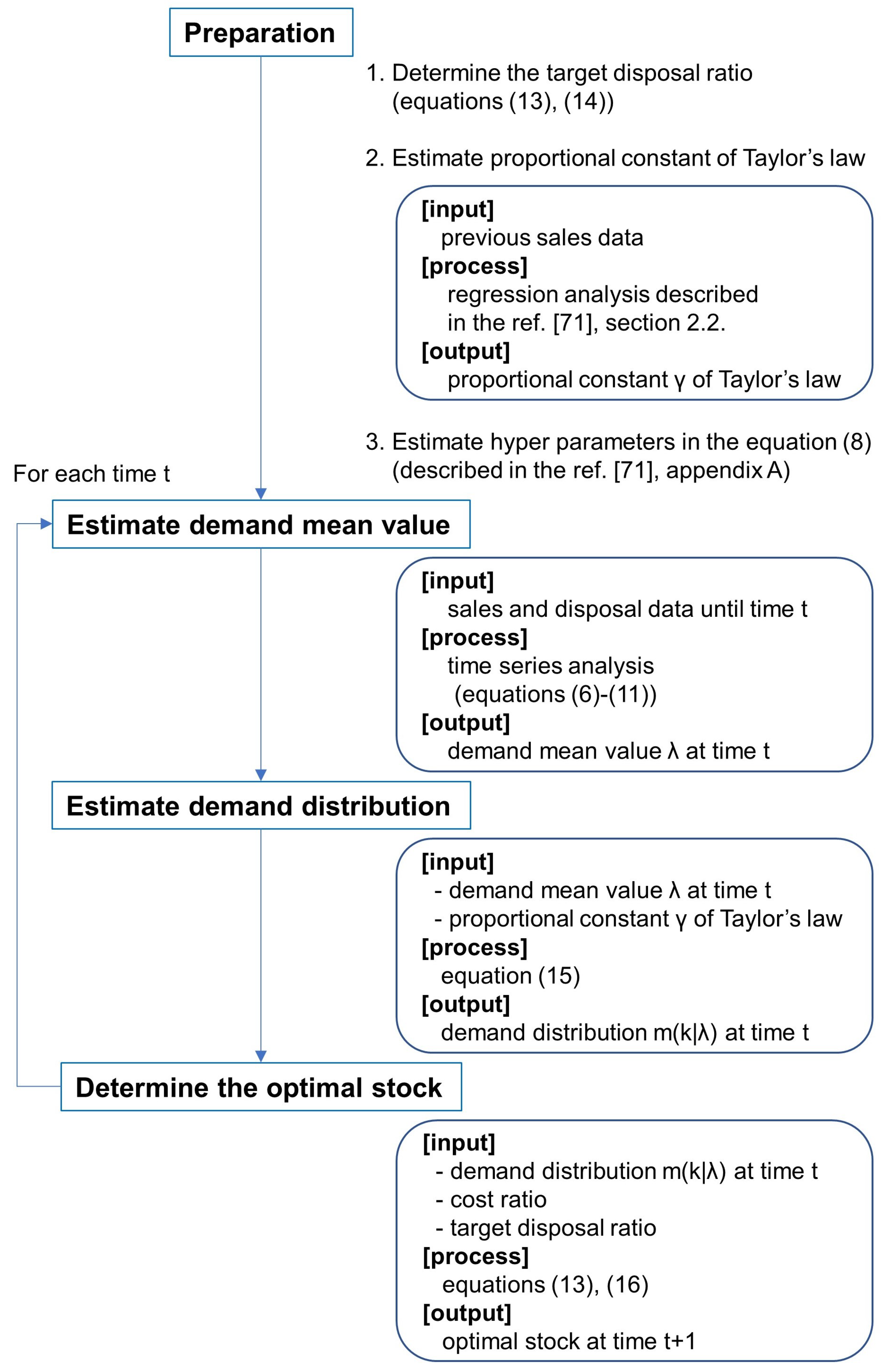
2.6. Summary of the Procedure to Determine the Stock

We summarize the procedure to determine the stock s ( α ) t with non-stationary and censored sales time series. Schematic diagram is shown in Figure 1.
  • Determine the target disposal ratio α with considering the cost of the waste reduction by the Equations (13) and (14). The proportionality constant γ of Taylor’s fluctuation scaling needs to be estimated empirically with the procedure described in the reference [71].
  • Set time t = 1 . The initial stock s 1 needs to be determined empirically. In this research, s 1 is calculated with the Equation (13) using sales value k 1 for simplicity.
  • Observe the sales k t and disposal d t of a product at time t. In the case of sold-out, the observed sales k t is the same value as the stock s t .
  • Estimate the demand mean value λ at time t with the SSM and the Particle Filter, namely Equations (6)–(11). In this estimation, the sales and disposal of the sales time series up to the day t is used.
  • Specify the demand distribution m ( k t | λ t ) at the day t with the Equation (15).
  • Determine the stock s ( α ) t + 1 with the Equations (13) and (16). Here, the demand mean value λ at time t + 1 is assumed to be equal to the λ at time t.
  • Inclement t = t + 1 and go back to step 3.
The verification of the method for estimating demand with censored sales time series and its effectiveness for determining the stock for each time is discussed in the Appendix A (Figure A2, Figure A3, Figure A4 and Figure A5).

2.7. Point-Of-Sales (POS) Data

The POS data are taken from 326 chain stores of a Japanese leading convenience store company, Seven-Eleven Japan Co., Ltd., during the 153 days from 1 June to 31 October 2010. The 326 stores are located in Kanagawa and Yamaguchi Prefecture in Japan. Individual owners mainly franchise the stores and sell extensive ranges of products, such as processed food, fast food, daily food, and non-food items including magazines, newspapers, stationeries, batteries, kitchen utensils, pet foods, liquors, and cigarettes. Sales of food items consist of 67.4% of total store sales and revenue from operations par shop a year was about 42 millions of Yen on average in 2010. The average floor space par shop is about 123 square meters [81].
The Pos data contains the record of each purchase at cash registers, and the daily amount of delivery and disposal for each shop and product. We obtained daily sales, delivery and disposal time series for each product in each store for the simulation of our method. We choose sales data of the food products which are disposed of more than 75% of sales days. There are two reasons for this selection. The first one is that our research aims to reduce food waste and verify the method can be applied to reduce an actual large amount of food waste. The other one is a technical reason for the verification of our method. The sales data with many sold-out days do not represent the underlying demand, which means the result of the demand estimation with our method cannot be verified, especially in the case when a higher demand than sales data is estimated with our method. The selected sales data are mainly on food items which are processed in the shops, such as fried chickens, frankfurter sausages and french fries. We limit the data to these items processed in the shops. Though these items are produced and disposed of several times a day, we aggregate production and disposal for each day for simplicity. The data with lost records in 153 days or unusual records because of promotions are excluded. We use 215 sales time series which are summarized in Table 1 for the simulation. The cost ratio is assumed to be 0.7, which is the typical value for the convenience store that is shown in the company’s investor relations [81].
The actual POS data with the record of disposal is rare in academic study. Though the POS data we possess is not the latest one, the statistical properties of sales data, namely, following the Poisson process and Taylor’s law, are universal and not time bounded. With difficulty in estimating fluctuating demand precisely, wastes from inappropriate stock management are assumed to occur all the same as formerly. Our POS data is qualified for the consideration of the method for waste reduction at present.

3. Results

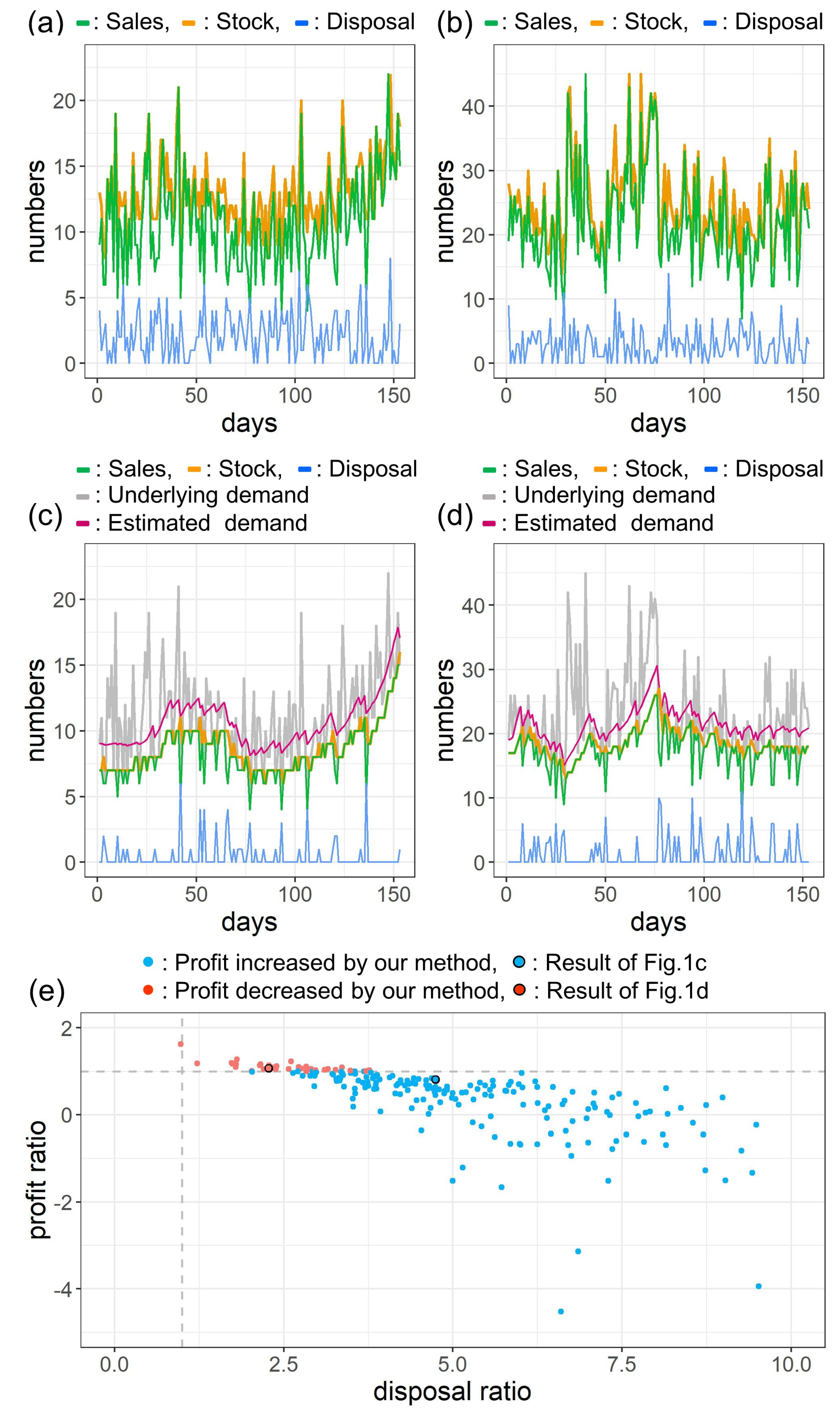
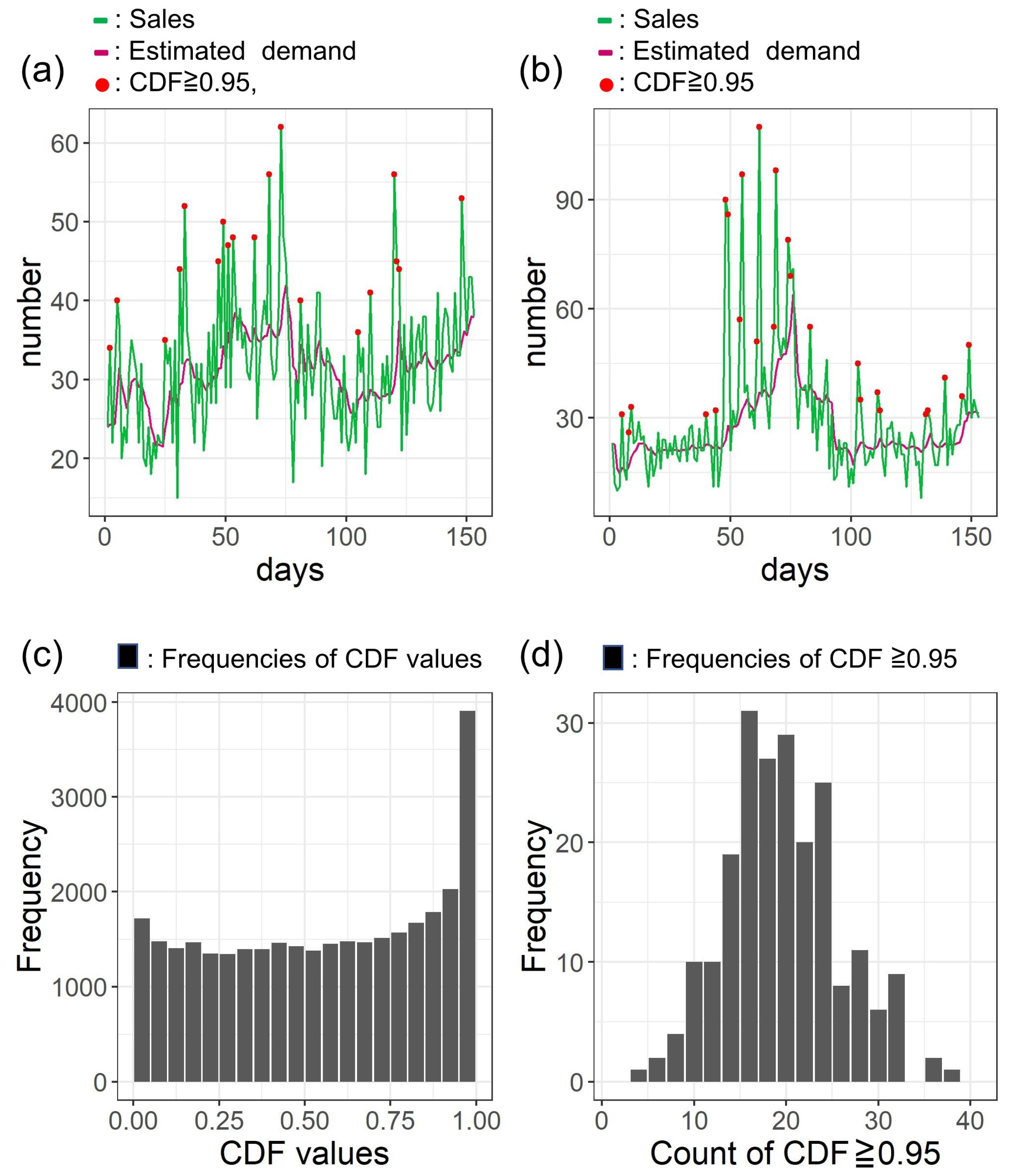
3.1. Optimal Stock Determination Using POS Data

Sales time series is generally non-stationary because of many factors such as weather condition and social trends. Figure 2a,b shows examples of daily sales number for fried chickens (fried chicken A in Table 1) in two shops. The green line indicates the sales. Non-stationary changes on demand are observed, such as the continuous rise after day 100 in Figure 2a, and the abrupt up-and-downs in Figure 2b. The orange line shows the stock and the blue line denotes the disposal for each day. In Figure 2a, the disposal are observed in 78% of 153 days. Specifically, 327 fried chickens in total are disposed of in 153 days. As for the profit, 1656 fried chickens in total are sold at 165 yen, so the amount of sales is 273,240 yen. The production cost of 1983 fried chickens is 229,037 yen (assuming cost ratio 0.7). Thus, the profit in the period is 44,203 yen. In Figure 2b, fried chickens are disposed of in 76% of 153 days, and the disposal amounts to 438 in total. The total profit is 117,068 yen since 3387 fried chickens are sold at 165 yen. Our method aims at the reduction of these large amounts of disposal with keeping a high profit by estimating non-stationary demand and determining the optimal stock for each day.
Figure 2c,d are the simulation results of our method using the same sales data as in Figure 2a,b. In this simulation, as we mentioned in the Methods Section 2.6, the stock at day t is determined with the sales and disposal of the sales time series up to the day t 1 . Specifically, we determine the mean of the demand at day t 1 with the time series analysis method described in the Section 2.3, namely Equations (6)–(11). In the case of sold-out, the potential sales number without sold-out is expected to be the same or more than the observed sales number. We estimate the likelihood of the demand when sold-out with the likelihood function for incomplete (censored) observation [79], namely Equations (10) and (11) in the Section 2.3, that take the expectation of more sales than stock into account. Assuming the demand at day t equals to the demand at day t 1 , the demand distribution at day t is determined with the Equation (15) in the Section 2.5. The optimal stock at day t is determined with the Equation (3) in the Section 2.1, using the demand distribution and the cost ratio. In Figure 2c,d, the gray line indicates the underlying demand. As the disposal are observed almost every day, we assume the sales can be regarded as the demand. The green line shows the observed sales, the orange line is the stock, the magenta line is the estimated mean of the demand and the blue line denotes the disposal. The disposal and the profit in Figure 2c are 69 and 54,599 yen, respectively. The disposal is reduced to 21.1% (69/327) and the profit is increased to 124% (54,599/44,204) with our method. In Figure 2d, the disposal is reduced to 43.9% (192/438) and the profit is decreased to 93.7% (109,692/117,068).
We applied our method to the 215 sales time series mentioned above. In each case daily stock is determined with the Equation (3) using sales and disposal time series up to the day. Figure 2e shows the profit and the disposal of shops for each 215 product, which is normalized as follows. We simulated the daily sales time series with our method for each 215 product, and obtained the total profit and disposal for each product. For comparison, we divide the profit and the disposal of shops by those of our method, respectively. The horizontal axis denotes the total disposal of a sales time series of a shop normalized by that of our method, and the vertical axis shows the total profit of a sales time series of a shop normalized by that of our method. The plots whose value exceed 1 in the horizontal axis, which is shown in the dashed gray line, correspond to the result that the waste amount simulated by our method is smaller than that of actual shops. The blue plots show the cases that the profit of our method is higher than that of real shops, and the red plots show the cases that our method gives lower profits. The results of Figure 2c,d are marked with black circles. We confirmed our method improved profit in 83.7% (180/215) of the plots. The negative value in the vertical axis corresponds to the negative profit of a shop, that results in the negative ratio of the profit. By aggregating the profit and the waste in Figure 2e, the waste of the shops (total amount of waste 103,468) is reduced to 23.2% (total waste 23,967), and the profit of the shops (total profit 8,255,002 yen) is increased to 140% (total profit 11,558,387 yen).

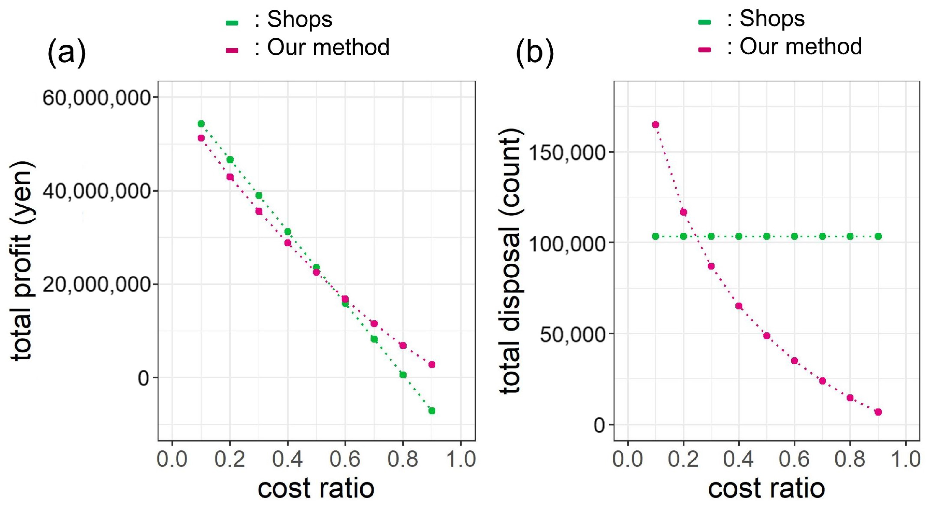
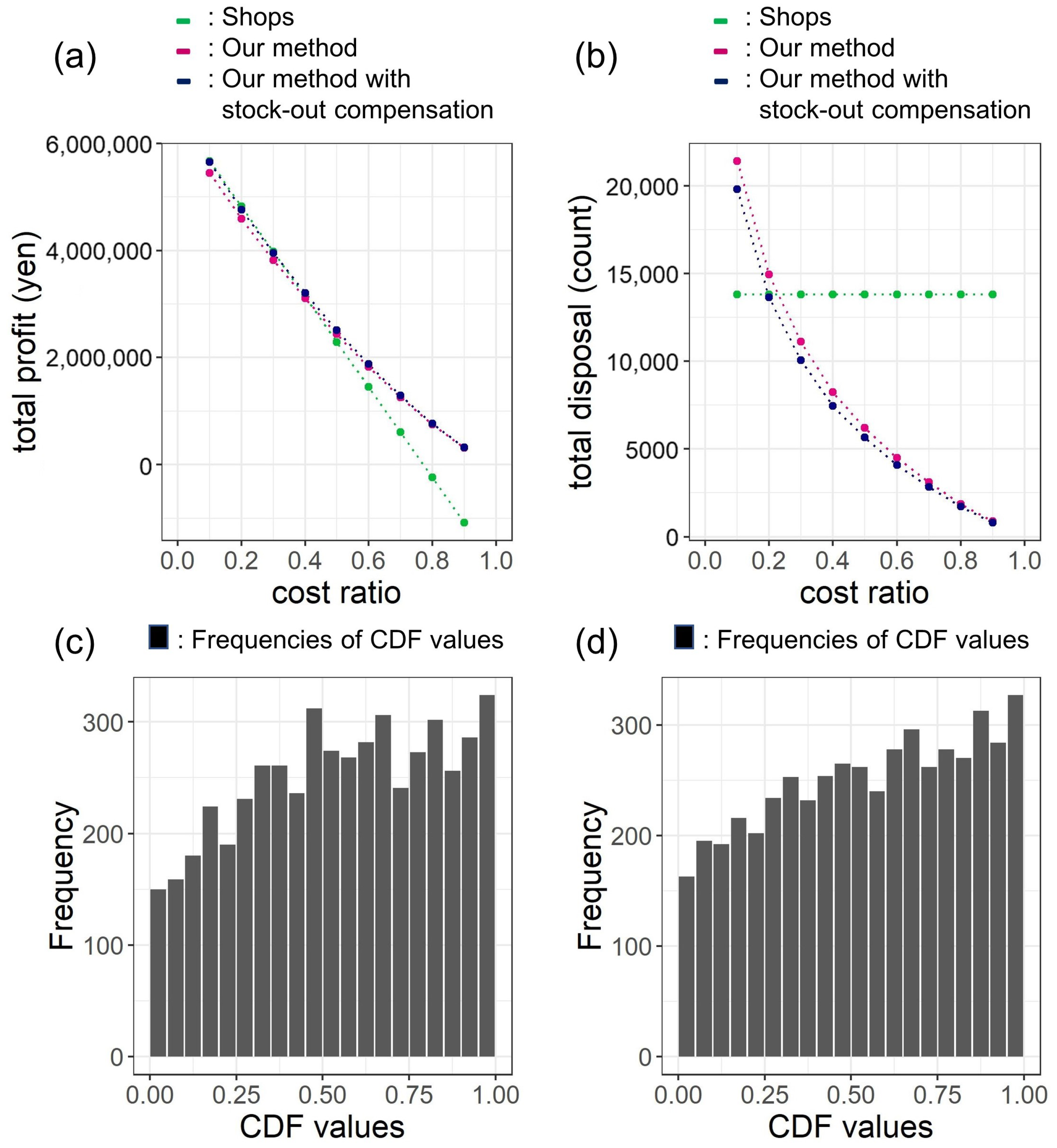
3.2. Further Waste Reduction

As we mentioned in the Section 2.4 and Section 2.5, our method provides a way to estimate the cost of waste reduction, which helps reduce waste further than the waste level shown in Figure 2e. Figure 3a shows the result of controlling waste reduction with estimating the cost. Each black plot represents the median and interquartile range of the profit and the disposal for each target disposal ratio from 0.5 to 0.9 assuming the waste level in Figure 2e is 1.0. Here, the Equation (13) is used to determine the daily stock. The dashed blue line represents the theoretical cost, namely profit loss, for the reduction of disposal, which is calculated with Equations (13) and (14). We confirmed that the food waste reduction by 27% is realized with 1% profit loss, and that of 45% is realized with 3.3% profit loss with this actual data.
In Figure 3a, the deviation between the target disposal ratio and the obtained disposal ratio is observed, such as the obtained disposal ratio 0.73 for target disposal ratio 0.7 and obtained disposal ratio 0.55 for target disposal ratio 0.5. Though the deviation is relatively small especially for a large target disposal ratio, we can empirically compensate for this deviation by regression analysis with the obtained and target disposal ratio. Figure 3b is the result of the regression analysis. The regression function is estimated to be g ( α ) = 1.09 α 0.09 , where g ( α ) is the target disposal ratio and α is the obtained disposal ratio. This function tells the disposal ratio α in the sales data analysis is obtained with target disposal ratio g ( α ) , so it can be used to compensate the target disposal ratio to obtain the desired disposal ratio in the sales data analysis.
The magenta plots in Figure 3a are the results using the compensated target disposal ratio g ( α ) , specifically from 0.455 to 1.0, to determine the optimal stock. We can see the deviation between the obtained and target disposal ratio is suppressed.
In the real shop operation, shop managers can estimate the regression function occasionally considering the deviation of the target and obtained disposal ratio. Besides, the regression function can be estimated in advance of the actual sales operation by using some artificial sales time series generated by random number simulation. The example of this estimation is shown in the Appendix A (Figure A6 and Figure A7).

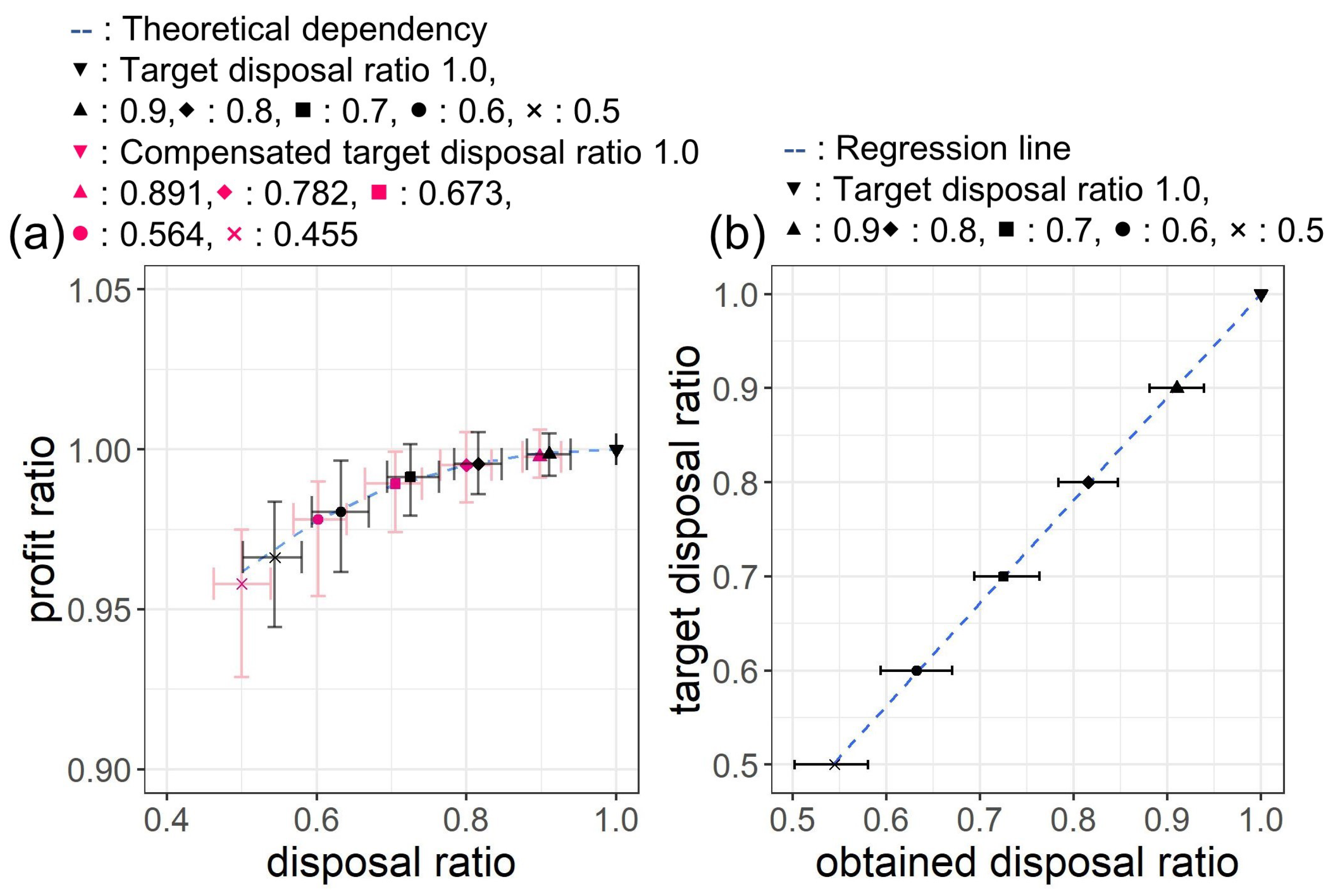
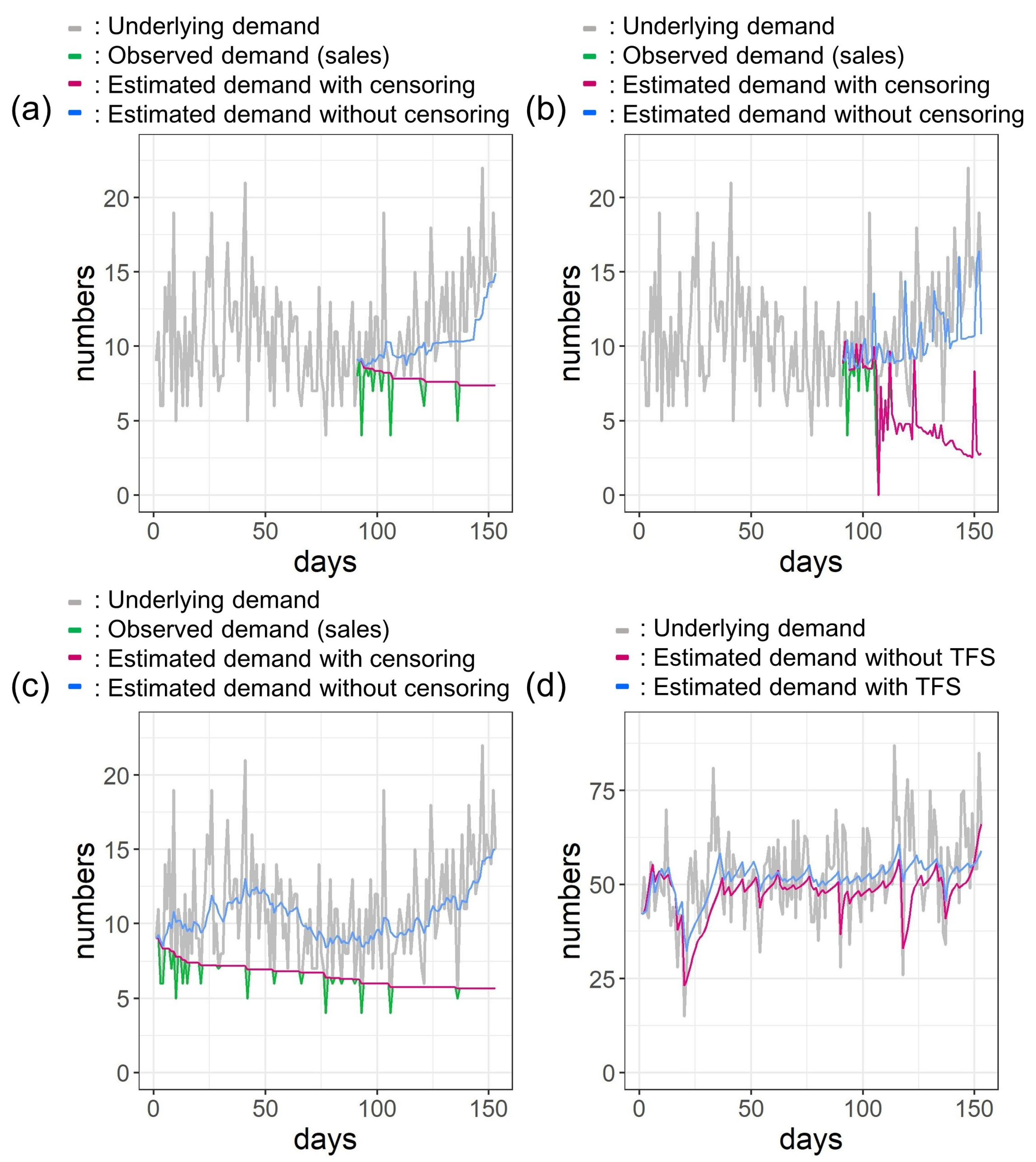
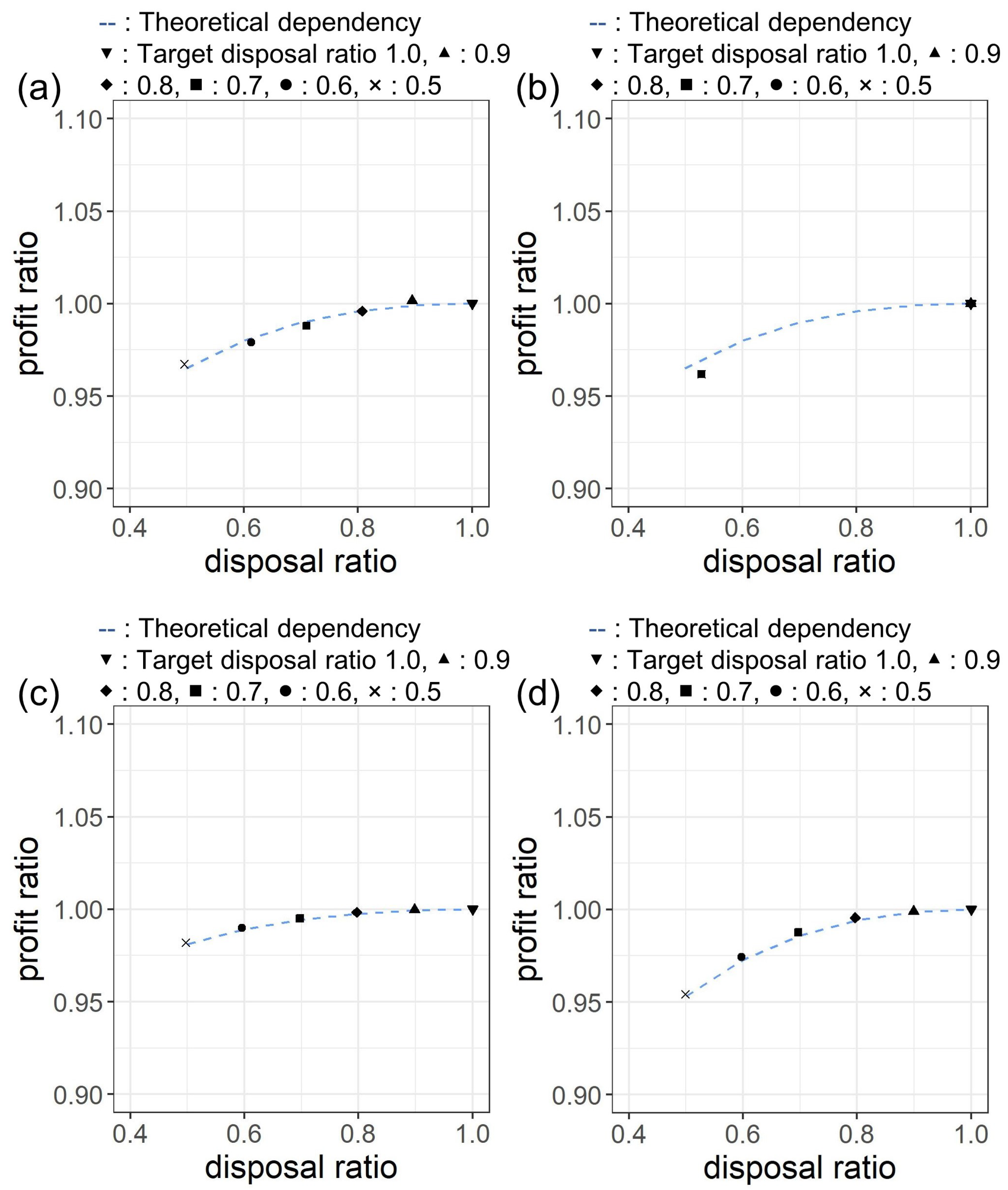
3.3. Detailed Examination on Our Method

We assume that the cost ratio is 0.7 which is the typical value of the convenience store [81]. Meanwhile, the cost ratio is supposed to be different for each food industry and product. As a small cost ratio allows a large amount of disposal for obtaining the same profit, the effectiveness of our method for various cost ratio should be examined. We examined the dependency of the profit and the disposal on the cost ratio with the 215 sales time series as a case study. The stock for each day is determined with the procedure described in the Section 2.6, and with the Equation (3) to determine the optimal stock as in Figure 2. Figure 4a is the estimated dependency of the total profit on the cost ratio. The green line denotes the total profit of the shops, and the magenta line shows that of the simulated result with our method. The total profit of our method is higher than that of the shops in the case that the cost ratio is above 0.55. Figure 4b is the total disposal of the shops (the green line) and that of our method (the magenta line). The disposal of our method is smaller than that of the shops above the cost ratio 0.25. At the cost ratio 0.55, the same profit as the shops and the waste reduced to 40.6% (42,016/103,468) compared to the shops are obtained with our method.
Figure 4a shows the profit of the shops surpasses that of our method below the cost ratio 0.55, whereas our method provides the optimal stock. One reason is that the sales data contains stock-out up to 25% of 153 sales days as mentioned in the Section 2.7. The increase in the profit with the optimal stock is supposed to be underestimated. We discuss this effect in detail later. Another reason is that there exist fluctuation that is not considered in our assumption. Figure 5a,b shows the examples of actual sales time series. The green line indicates sales and the magenta line denotes the estimated demand mean, assuming the cost ratio 0.1. We examine the probability of each sales data realized by the assumed demand distribution, namely the Equation (15). The red plots indicate that the value of Cumulative Distribution Function (CDF) of the sales value realized by the demand distribution is greater than or equal to 0.95. These peaks with CDF greater than or equal to 0.95 appear more than theoretically expected. Figure 5c shows the histogram of the CDF values for each sales in the 215 sales time series. Though the frequencies of CDF values are to be uniform if the assumed distribution fits the sales data, the frequency of CDF greater than or equal to 0.95 is more than two times larger than that of other bins of the histogram. Figure 5d is the histogram of the count of CDF greater than or equal to 0.95 in each 215 sales time series. The theoretical realization probability of CDF greater than or equal to 0.95, for 15 days in 153 days is 1.0%. But 84.2% of the sales time series show the CDF values more than or equal to 15 days. One of the sales time series contains sales peak over 100 σ . These peaks are supposed to arise from some irregular reasons such as bulk orders for events. Since shops cover these abrupt sales peaks which occur with very low probability, some prior knowledge or notification in advance of the sales peaks might have been provided somehow to the shop.
To discuss the potential of our method, we remove the abnormal sales time series whose count of CDF greater than or equal to 0.95, are observed more than or equal to 15 days. A sales time series with a peak over 100 σ is also removed. Figure 6a,b are the estimated dependency of the profit and the disposal on the cost ratio with the 33 sales time series obtained. The green line is the result of shops, and the magenta line denotes that of our method. The navy line illustrates the result of our method with compensation of the sales underestimation because of the stock-out. Here we calculate the expected sales in stock-out days using the Probability Density Function (PDF) of the demand distribution, namely the Equation (15). Specifically, we get the expected sales above the stock for each sold-out day by calculating the sum product of the PDF and sales count greater than or equal to the stock, and devide the obtained value by the summation of the PDF whose sales count greater than or equal to the stock. Then, we compensate the sales for each sold-out days up to disposal count at the day. In Figure 6a, we can see the compensated profit of our method (the navy line) approaches asymptotically to that of shops (the green line) as the cost ratio decreases. In Figure 6b, the compensated disposal of our method (the navy line) decreased compared to the original disposal of our method (the magenta line) since the additional sales by the compensation decrease the disposal.
Figure 6c shows the histogram of CDF with the 33 sales time series. The excessive count of CDF greater than or equal to 0.95 is suppressed. Since the data size is relatively small, the histogram appears not to be uniform. To see the consistency with the result and the theoretically expected frequency, we simulated the theoretical histogram with random numbers whose distribution follows Equation (15) and each demand mean is the estimated values for each 33 sales time series. Figure 6d denotes an example of the simulated theoretical histogram, which shows a similar tendency with the result of actual sales data. We confirmed the equivalency of the theoretical and the actual distribution with Kolmogorov–Smirnov test. Namely, the p-value comparing the CDF distribution obtained with the actual sales data, and that of random number simulation, repeated 200 times with changing random number seed, is 0.07 on average, which shows the difference of the theoretical and the actual distribution of the CDF is not statistically significant at the p-value 0.05.
Figure 6a tells the profit and the disposal with our method compared to shops are equivalent at the cost ratio 0.2, and the disposal 59.7% (8247/13,822) with the same profit compared to shops are obtained at the cost ratio 0.4. At the cost ratio 0.7 which is typical for the convenience store, the profit is 208.0% (1,260,691/606,070 yen) and the disposal is 22.4% (3097/13,822) compared to the shops.

4. Discussion

As we mentioned in the Introduction section, some methods are already proposed for demand estimation. Here, we examine the conventional methods and clarify the advantages of our method.
BDP and some related heuristics [35,36,37,40,41,42,43] are developed for demand estimation and stock management under demand uncertainty and censoring. Meanwhile, BDP for non-stationary demand is not proposed [51], except for the recent research which proposes BDP for demand (without censoring) with a single change point [56]. Non-parametric methods proposed for demand estimation and stock management [47,48,49,50] also assume stationary demand. Developing these methods for non-stationary demand is one of the open research areas [51].
MDD, ARIMA and NN are applicable to non-stationary demand. In these methods, MDD proposed in the literature [52,53,54,55] assume the transition probability matrix and the demand distribution within each Markov state is known and fixed. This assumption limits the practicability since non-stationarity is usually unpredictable. ARIMA [57,58,59,60] and NN [62] can be used to non-stationary demand with underlying patterns such as auto-correlation and seasonality. However, the underlying patterns may change with such factors as the social trend and weather condition. Moreover, MDD, ARIMA and NN are not ready for handling censored sales data.
One may think of a more simple non-stationary time series analysis method, Moving Average and their family, such as Exponentially Weighted Moving Average (EWMA) [82]. These smoothing methods are also not applicable to censored sales data.
We examine above mentioned methods which are applicable to a non-stationary sales time series, namely ARIMA, NN and EWMA. In these methods, ARIMA and NN are executed with the statistics software R, specifically the software packages f o r e c a s t and n n e t , respectively. EWMA is implemented as D t = α Y t 1 + ( 1 α ) D t 1 , where D t is estimated demand for day t, Y t 1 is sales data at day t 1 and α is the smoothing constant [82].
Here, we explain the procedure of the examination. The POS data shown in Figure 2c is used for the examination. As ARIMA and NN require training data, the demand data within the initial 90 days are used for initial training and no censoring is considered in this training data. For each day from day 91, all previous data up to the day is used for retraining the ARIMA and NN model. The demand for the next day is predicted with the model. For simplicity, the stock for each day is determined as the same value as the predicted demand, that is equivalent to the case where the cost ratio is 0.5 for a symmetric demand distribution.
Specific ARIMA model for each day is determined to be ( p , d , q ) = ( 0 , 1 , 1 ) with Akaike Information Criterion (AIC) [83], where p is the order of AR, d is the degree of differencing and q is the order of MA [57]. As for the NN model, the number of neurons in the hidden layer is set to be 10. As a large number of neurons results in overfitting and instability of the estimation, while small number leads to underfitting, we select one of the balanced condition that can generally follow the trend with stability.
As EWMA needs no training, daily demand is estimated from day 2 with the EWMA equation. D 1 is assumed to be Y 1 and the value of α is set to be 0.12 with try and error to follow the trend.
Figure 7a–c is the result of demand estimation with ARIMA, NN and EWMA, respectively. The gray line indicates underlying demand. The blue line shows the estimated demand with sales data without censoring, and the magenta line shows that with censoring. The estimated demand without censoring generally follows the trend. Meanwhile, the estimated demand with censoring fails to follow the trend. Using censored sales data without any compensation results in an underestimate of the underlying demand.
Since these conventional time series analysis and machine learning are not ready for censored demand, some exogenous compensation of censoring is needed for demand estimation with censored sales data, such as compensation with intuition, experience or considering some patterns in sales. Our method compensates the censored demand with the statistical likelihood, namely Equation (11), and needs no exogenous compensation. To our knowledge, our approach firstly provides practical solutions for non-stationary and censored demand estimation.
As the examination within our method, we compare the model with and without considering Taylor’s fluctuation scaling (TFS). Figure 7d is the result of demand estimation with and without considering TFS. Note that demand λ in Figure 7d is relatively large (i.e., λ > 20 ), so Taylor’s fluctuation scaling is assumed in the sales data. The blue line denotes the demand estimation with TFS, specifically the Equation (9) is used for the estimation. The magenta line indicates the demand estimation without TFS, namely only Poisson distribution in the Equation (9) is assumed. The estimated demand without TFS is smaller than that with TFS. We confirmed the profit obtained without TFS is 3.3 % smaller than that with TFS. As shown in the reference [71], large fluctuations caused by TFS are regarded as non-stationary changes if TFS is not considered in the conventional Poisson model. Unlike large values, small values of the demand distribution are observed under censoring. These small values are considered as non-stationary changes in the Poisson model, which lowers the estimation.

5. Conclusions

The non-stationary parameter estimation method based on Particle Filter which considers Taylor’s fluctuation scaling is extended for demand estimation with censored sales data. By combining this method with the newsvendor problem formula to determine the optimal stock, reduction of food waste keeping high profit is realized. The extension of the newsvendor problem formula to examine the relationship between the amount of waste and profit provides new insights into the cost of waste reduction.
The retail shops handle many products and have to determine the stock for each product for each day. For example, the convenience stores generally deal with over 500 food products which require disposal management considering the expiration date. Our method helps retailers estimate the non-stationary demand and determine the optimal stock for each product for each day, which enables reducing food waste with keeping a high profit in the real activity. The stock determination with intuition [66] or constant inventory level that result in a large amount of waste can be avoided by our method.
Meanwhile, multilateral managerial viewpoints, especially constraints such as internal factors (lack of space, infrastructure, etc.), human capital factors(lack of time or staff, motivations, skills, etc.), external factors(uncollaborative customers, suppliers, etc.) and legal factors(local legislation, etc.) are needed to be considered for practical implementation [30]. As for the internal, external, and legal factors, our method is accessible to ordinary retail stores. The method is based on data analysis on a personal computer. More concretely, the data used in our method is sales data of the shop itself. Furthermore, the data analysis requires no sizeable computational resource such as a large server or cloud computing. Namely, our method can estimate the demand for 153 days of a product in a few seconds with a personal computer for consumer use (i.e., Intel Core i5-6400 2.7GHz CPU and 16GB Memory). Short computational time is important since ordinary shops are not necessarily accessible to huge computational resources and have to manage stocks for many products.
In the factors mentioned above, human capital factors, specifically, the requirement for some Information Technology (IT) and data science knowledge, can be a barrier to the introduction of our method. Human resources who are knowledgeable of IT and data science are not sufficient worldwide. Providing some computer software or online platform that is easy to use without programming skills, along with holding some hands-on seminars, could be a realistic solution for implementation. Some other factors, such as perception in retail managers that stock-out leads to lost not only sales but also the loyalty of the customer [66] could be an obstacle since our method could increase stock-outs by eliminating over-stocking. Awareness campaigns for managers as well as consumers to change the perception of stock-out might be required. Low recognition of technologies and reluctance of retail managers to adopt IT tools [30] should also be addressed. We need to accumulate successful cases and present the merit properly. Such cultural barriers as a lack of consumer interest and awareness as well as a hesitant company culture are also considered to be the primary obstacles in the case of promoting the circular economy [84]. As a long time measure, policies to increase the experts on IT and data science who can make full use of the company’s data is also essential since scientific consideration based on data, which is not limited to the proposed method, should realize effective measures for food sustainability.
Financial issues for implementing green innovations should be carefully examined. In the case of innovations which require a substantial amount of investment, financial actors such as banks, venture capitals, business angels, and private investors play an important role. Recent researches reveal relationships between the types of funding and innovations for renewable energy [85], the pressures of various financial actors in the greening of the financial system in Italy [86], and factors that prevent investment decisions of green companies in biomass production sector [87]. Financial sustainability in cases of waste management of municipalities is also discussed [88]. Since retailers now work on green innovations mainly in their operational processes and technologies available, taking advantage of investments from green finance to overcome financial issues is not reported in surveys on the actual waste reduction practices in retail [24,30]. Our method needs the initial cost of introducing software that is not supposed to require a substantial amount of investment as the cases of biomass and renewable energy. Meanwhile, a small amount of investment could be an obstacle for small shops. Promoting green finance for small-scale investment needs, which is reported to be scarce [87], could help spread our method and other green innovations in retail.
As for the technical aspects, we demonstrated an approach to verify the consistency of the assumed statistical model and the actual sales data using CDF in the Section 3.3. Specifically, we obtained a CDF histogram which corresponds to the realization probability of sales value by the assumed demand distribution. This CDF histogram tells mismatch between the assumed model and actual data. Besides its information can be used to remove the abnormal data, it can be used to modify the statistical model.
There exist limitations and rooms for future research in our method. Periodicities in sales time series such as weekly cycle and seasonality that are specific for each type of industry and product are not included in our model. If the systematic deviations because of periodicities are substantial, taking such periodicities into account in our model may yield better accuracy of the demand estimation. We assume a constant price for each product. Retailers reduce the price of foods which are approaching their expiry date. Incorporating pricing decisions into the model makes the model more efficient. Demand substitution which expects to mitigate the stock-out effect is not considered in our model. Understanding the interaction for each sales amount of product considering stock-out, and incorporating this knowledge into the model may lead to further waste reduction.
The adjustment of Taylor’s scaling factor γ in the Equation (4), which governs fluctuation of the demand distribution, may contribute to the estimation accuracy. Statistically, the correlation of the underlying population (customers) causes Taylor’s scaling exponent takes a value between 0.5 and 1.0 whereas the Equation (4) assumes the scaling exponent to be 1 (linear). Some examples of the scaling exponent below 1 are found in non-food products on the POS data, such as stamps which are often purchased in bulk and magazines that are specifically bought on the launch day [73]. Influence of a TV program or social trend may cause the correlation of customers for food products. In the future work, the modification of Equation (4) corresponding to the scaling exponent below 1 will provide a more general form of our method.
Our method provides practical solutions for estimating non-stationary and censored demand. The method has the potential to apply to sales data of other sectors than retail, specifically, food manufacturing and supplying industry, and food service sectors such as restaurants, cafeterias, and catering services since the property of the sales data, that follows Poisson process and Taylor’s law, is assumed to be universal.

Author Contributions

Conceptualization, G.S., H.T. and M.T.; Data curation, G.S.; Formal analysis, G.S.; Funding acquisition, M.T.; Investigation, G.S.; Methodology, G.S., H.T. and M.T.; Project administration, H.T. and M.T.; Resources, M.T.; Software, G.S.; Supervision, H.T. and M.T.; Validation, G.S.; Visualization, G.S.; Writing—original draft, G.S.; Writing—review and editing, H.T. and M.T.

Funding

This work was partially supported by JSPS KAKENHI (Grant No.18H01656).

Acknowledgments

The authors would like to thank Seven-Eleven Japan Co., Ltd. for providing the POS data.

Conflicts of Interest

The authors declare no conflict of interest.

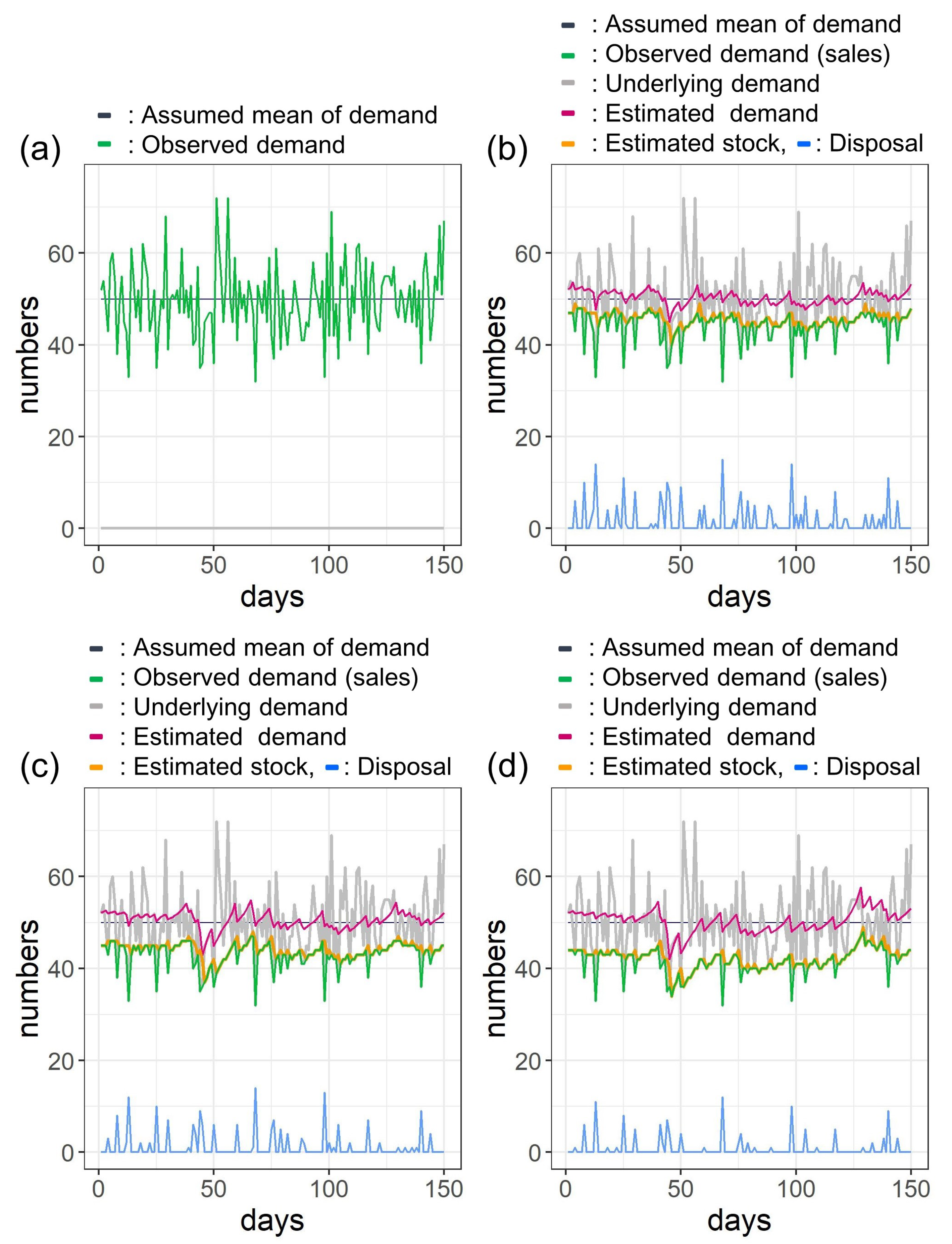
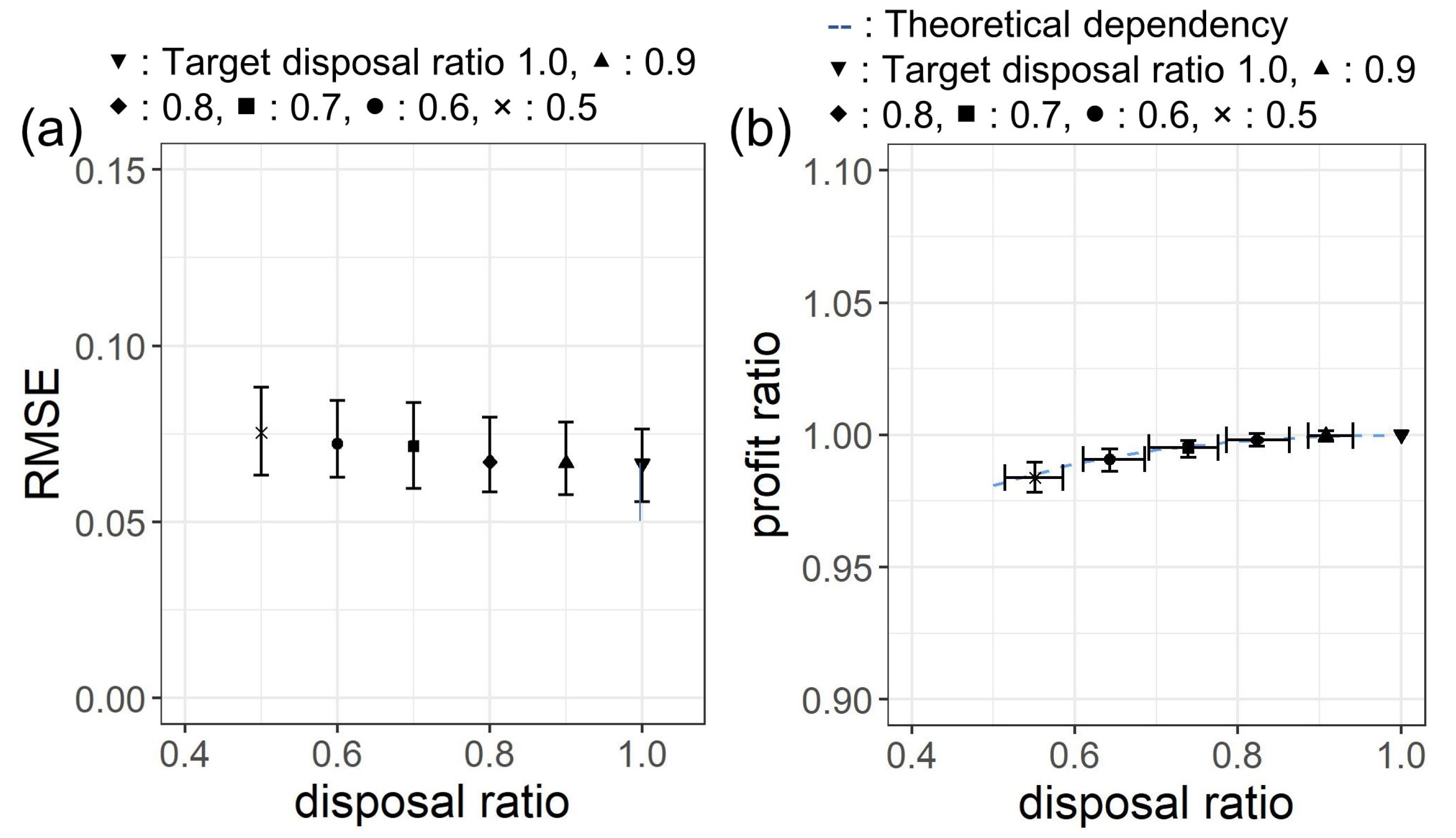
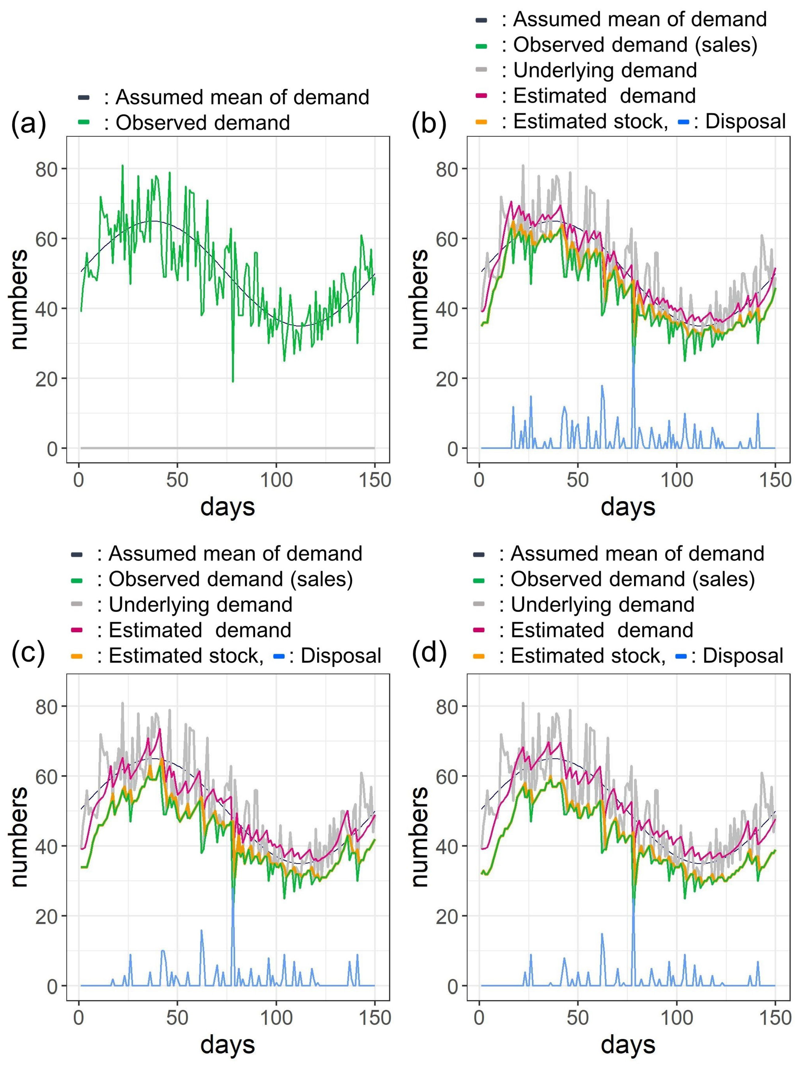
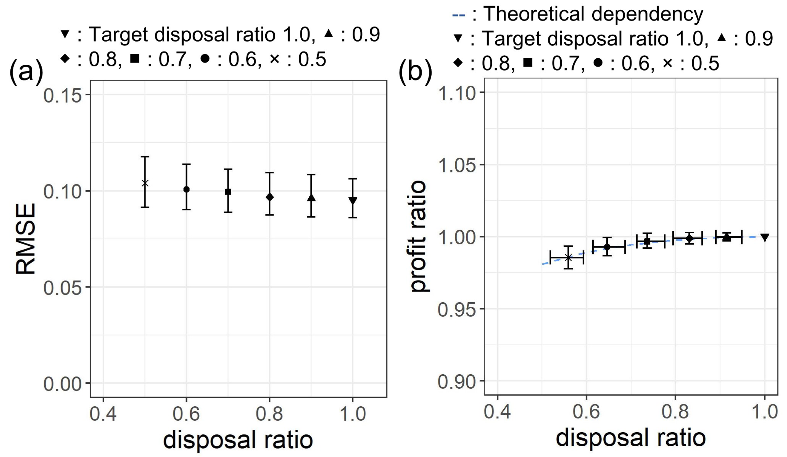
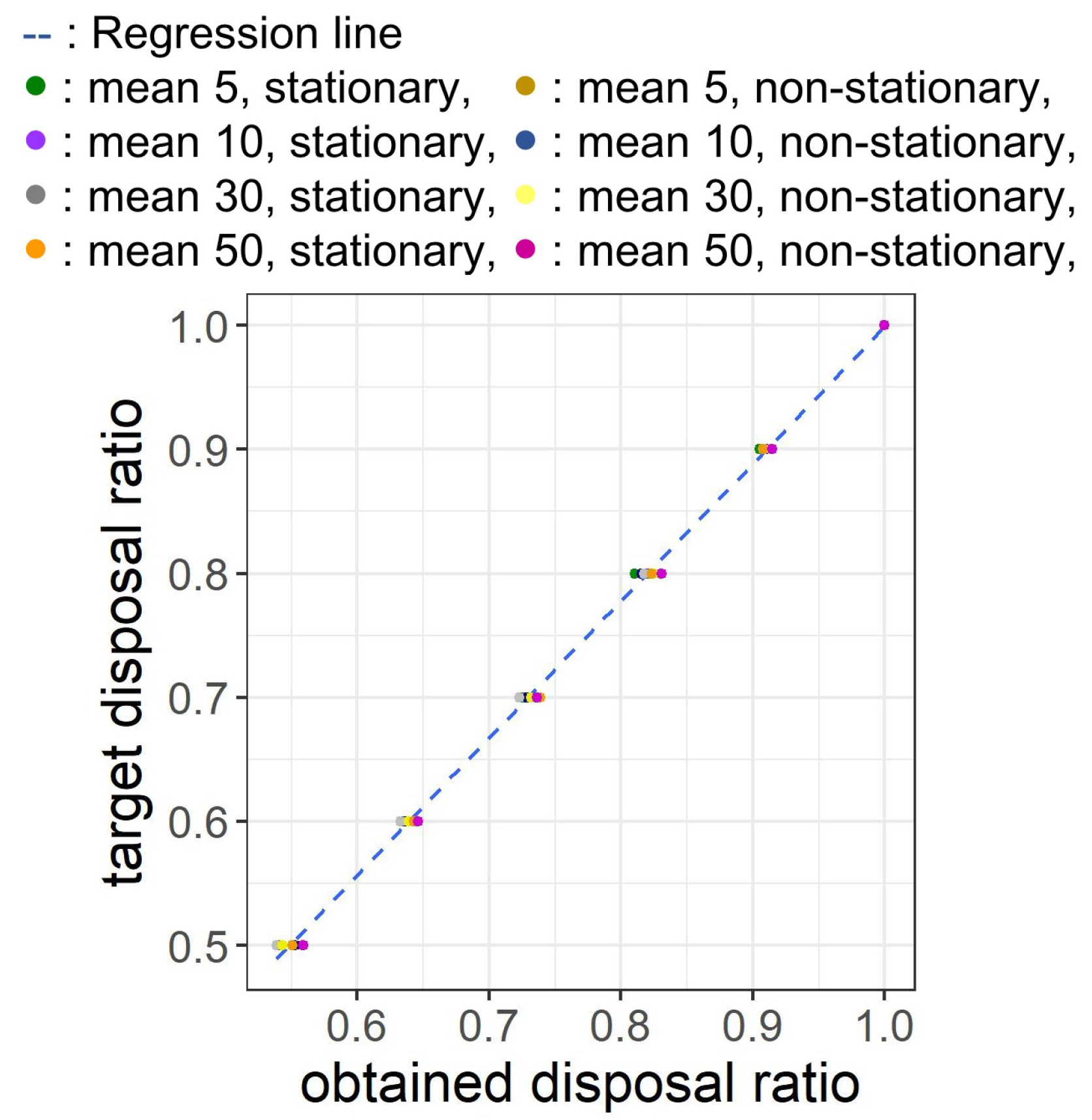
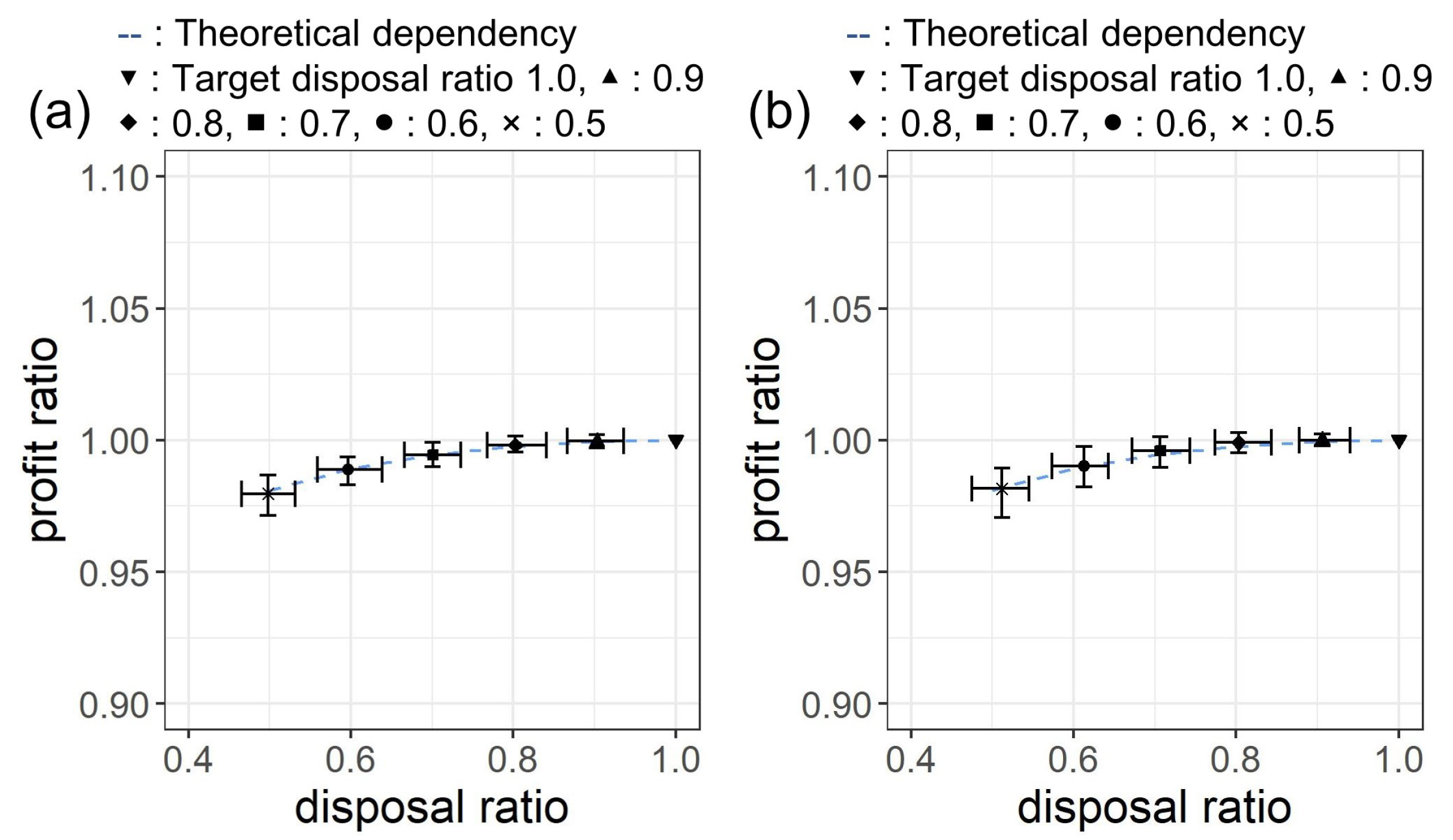
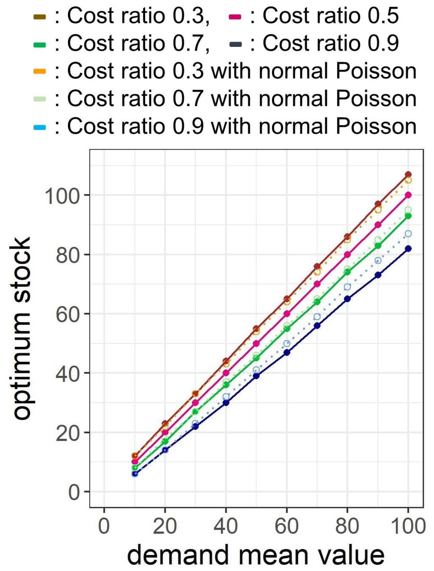
Appendix A. Verification of Our Method with Artificial Time Series

We verify our method with artificial time series generated by random number simulation. There exist two components to confirm in our method. The first one is the accuracy of the estimated dependency between the disposal and the profit with the Equations (13) and (14). The other one is the time series analysis method based on the SSM and the Particle filter, for estimating demand with incomplete (censored) sales data because of sold-out, and its effectiveness for determining the stock for each time. We examine these in this section.
First, we verify the accuracy of the estimated dependency between the disposal and the profit. The artificial demand time series is generated with assuming the PDF of demand shown in the Equation (5). The stock values for the target disposal ratio between 0.5 to 1.0 are calculated with the Equation (13). By comparing the demand time series and the stock value, the number of sales and disposal for each time are obtained. The profit is calculated assuming the cost ratio 0.7 and the price 1. Figure A1a illustrates the result of the profit and disposal, assuming the mean of the demand is 10, and 10,000 random numbers for demand time series. Each plot denotes the profit and the disposal for each target disposal ratio from 0.5 to 1.0. The dashed blue line is the theoretical dependency of the disposal and the profit obtained with the Equations (13) and (14). We can see the obtained values of the profit and the disposal fit well to the theoretical dependency.
The specific stock values for the target disposal ratio between 0.5 and 1.0 are between 7.10 and 8.22. These stock values in the form of real value, instead of integer value, are obtained with the Equation (15), namely Poisson distribution modified with the Γ function to handle a real value. Since the stock value in reality should be an integer, we use the probabilistic determination of the stock shown in the Equation (16) to approximately reproduce the real number of the target stock with discrete stock values. Figure A1b shows the result with normal Poisson distribution shown in the Equation (5), and without the probabilistic determination of the stock, that results in poor controllability of the disposal and the profit.
In our study, the fluctuation of the demand distribution is assumed to follow Taylor’s fluctuation scaling shown in the Equation (4). Thus, the mean value of the demand and the proportionality constant of Taylor’s fluctuation scaling govern the demand distribution. Figure A1c,d are the results of the estimated profit and disposal, assuming the mean of the demand is 50, and 10,000 random numbers for demand time series. The proportionality constant of Taylor’s fluctuation scaling is assumed to be 0.1 for Figure A1c, and 0.3 for Figure A1d. Each result shows the obtained profit and disposal fit well to the theoretical dependency. The effectiveness of our approach for estimating the dependency of the disposal and the profit is confirmed.
Next, we verify the time series analysis method based on the SSM and the Particle filter, for estimating demand with incomplete (censored) sales data because of sold-out, and its effectiveness for determining the stock for each time t.
Figure A1. Profit and disposal for each stock corresponding to target disposal ratio between 0.5 to 1.0, estimated with 10000 random numbers as demand time series. (a) Result for the demand mean 10. (b) Result for the demand mean 10, where the stock is estimated with normal Poisson distribution, and without the probabilistic determination of the stock. (c) Result for the demand mean 50 and the proportionality constant of Taylor’s fluctuation scaling 0.1. (d) Result for the demand mean 50 and the proportionality constant of Taylor’s fluctuation scaling 0.3. The dashed blue line denotes the theoretical dependency of the disposal and the profit obtained with the Equations (13) and (14).
Sustainability 11 03589 g0a1
Figure A2a is an artificial demand time series assuming the mean value of the demand is 50, and the proportionality constant of Taylor’s fluctuation scaling is 0.1. The green line denotes the demand and the navy line is the assumed mean value of the demand. Figure A2b illustrates the simulated sales time series by our method, in which the stock value for each time t + 1 is determined based on the estimated demand at time t. The stock value is estimated with the Equation (3), that is, the target disposal ratio equals to 1.0. The gray line indicates underlying demand, the green line denotes observed sales, the blue line is disposal, and the magenta line is the estimated mean value of the demand. Since the optimal stock estimated with the Equation (3) is generally under the mean of the demand, the observed sales are often censored at the stock value which can be confirmed in the zero values of disposal in the blue line. The estimated mean value of the demand in the magenta line is around 50 that is the assumed value of the mean of the demand. Figure A2c,d are the simulated sales time series assuming the target disposal ratio 0.7, 0.5, respectively. Although the deviation of the estimation value becomes larger in accordance with the decrease in the target disposal ratio, the estimated mean values of the demand are around the assumed demand value 50.
Figure A2. Verification of the time series analysis method for the stationary demand. (a) Artificial stationary demand time series assuming the mean value of the demand 50, and the proportionality constant of Taylor’s fluctuation scaling 0.1. (b) Simulated sales time series with our method assuming the target disposal ratio 1.0. (c) Simulated sales time series with our method assuming the target disposal ratio 0.7. (d) Simulated sales time series with our method assuming the target disposal ratio 0.5. The navy line is the assumed mean of the demand, the green line denotes the observed demand, the gray line means the underlying demand, the magenta line indicates the estimated demand mean, the orange line shows the estimated stock and the blue line illustrates the disposal.
Sustainability 11 03589 g0a2
We quantitatively examine the precision of the demand estimation, and the accuracy of the estimated dependency of the disposal and the profit. Considering the deviation of the random numbers and that our method adopts the probabilistic determination of the stock, we check the tendency with 200 sets of random number demand time series. The mean value of the demand is set to 50, the proportionality constant of Taylor’s fluctuation scaling is assumed to be 0.1, and 150 random numbers are generated for each demand time series. Figure A3a shows the Root Mean Squared Error (RMSE) between the estimated and the assumed mean value of the demand. Each plot denotes the median and the interquartile range of the RMSE for each target disposal ratio. The RMSE increases following the decrease in the target disposal ratio, namely, 6.6% RMSE for target disposal ratio 1.0 and 7.5% RMSE for target disposal ratio 0.5. It is because the decrease in target disposal ratio leads to an increase in censoring (stock-outs) because the stock value decreases, that makes precise demand estimation difficult. Figure A3b shows the median and the interquartile range of the estimated disposal and profit for each target disposal ratio. Each plot fits the theoretical dependency of the disposal and the profit shown in the dashed blue line, obtained with the Equations (13) and (14).
Figure A3. Examination on the precision of estimating the stationary demand and the dependency of the disposal and the profit. (a) Median and interquartile range of the Root Mean Squared Error (RMSE) between the estimated and the assumed mean value of the demand. (b) Median and interquartile range of the estimated disposal and profit for each target disposal ratio.
Sustainability 11 03589 g0a3
We verified our method for a non-stationary time series. Figure A4a shows the demand time series with a sine curve shape, with the mean value 50, the amplitude 30 and the periodicity 150. The proportionality constant of Taylor’s fluctuation scaling is assumed to be 0.1. The green line is the demand and the navy line is the assumed mean of the demand. Figure A4b–d are the simulated sales time series created with the same procedure as Figure A2b–d. The estimated mean value of demand in the magenta line follows the assumed non-stationary demand in the navy line for each target disposal ratio 1.0, 0.7, 0.5, respectively. Figure A5a is the RMSE between the estimated and the assumed mean value of the demand. The RMSE increases with the decrease in the target disposal ratio as seen in Figure A3a. Figure A5b is the median and the interquartile range of the estimated disposal and profit for each target disposal ratio. Each plot fits the theoretical dependency of the disposal and the profit shown in the dashed blue line as in Figure A3b.
The obtained disposal in Figure A3b and Figure A5b deviate in a few percents from the target disposal following the decrease in target disposal ratio. This deviation can be compensated with a regression function estimated with the target and the obtained disposal ratio. Along with using the result of the target and the obtained disposal ratio in Figure A3b and Figure A5b, we can estimate the regression function with results of the target and the obtained disposal ratio for various demand mean values, with a view to obtaining more general form of the regression function and applying it to the actual sales data analysis. Figure A6 is an example of the regression analysis. Each plot represents the result of the target and the obtained disposal ratio, which is calculated with stationary and non-stationary demand time series. The demand mean values are assumed to be 5, 10, 30, 50. For the non-stationary demand time series, a sine curve shaped demand is assumed which amplitude is 60% of the mean value. In the Figure A6, the green plot is the result of the demand mean 5 and stationary time series. As for the other plots, with stationary time series, the purple plot is for the demand mean 10, the gray plot is for the demand mean 30 and the orange plot is for the demand mean 50. With non-stationary time series, the brown plot is for the demand mean 5, the navy plot is for the demand mean 10, the yellow plot is for the demand mean 30 and the magenta plot is for the demand mean 50. The dashed blue line denotes the estimated regression line, g ( α ) = 1.11 α 0.11 , where α is the obtained disposal ratio and g ( α ) is the target disposal ratio, which tells disposal ratio α is obtained with target disposal ratio g ( α ) . This function can be used to estimate the compensated target disposal ratio g ( α ) to obtain desired disposal ratio α . We calculated the disposal and the profit using the compensated target disposal ratio g ( α ) . Figure A7a is the result for the stationary demand with the same data as Figure A3b, and Figure A7b is the result for the non-stationary demand with the same data as Figure A5b. In Figure A7a,b, the plotted disposal and the profit for each target disposal ratio (from 0.5 to 1.0) is the result using the compensated disposal ratio g ( α ) , specifically from 0.445 to 1.0. We can see the deviation between the obtained and target disposal ratio is suppressed.
Figure A4. Verification of the time series analysis method for the non-stationary demand. (a) Artificial non-stationary demand time series assuming the mean value of the demand 50, and the proportionality constant of Taylor’s fluctuation scaling 0.1. (b) Simulated sales time series with our method assuming the target disposal ratio 1.0. (c) Simulated sales time series with our method assuming the target disposal ratio 0.7. (d) Simulated sales time series with our method assuming the target disposal ratio 0.5. The navy line is the assumed mean of the demand, the green line denotes the observed demand, the gray line means the underlying demand, the magenta line indicates the estimated demand mean, the orange line shows the estimated stock and the blue line illustrates the disposal.
Sustainability 11 03589 g0a4
Figure A5. Examination on the precision of estimating the non-stationary demand and the dependency of the disposal and the profit. (a) Median and interquartile range of the Root Mean Squared Error (RMSE) between the estimated and the assumed mean value of the demand. (b) Median and interquartile range of the estimated disposal and profit for each target disposal ratio.
Sustainability 11 03589 g0a5
Figure A6. Regression analysis of the obtained and target disposal ratio. Each plot represents the median of the target and obtained disposal ratio calculated with 200 set of 150 random number time series with demand mean value 5, 10, 30, 50, with stationarity and non-starionarity (sine curve, amplitude 30%, period 150). The green plot is demand mean 5 and stationary, the brown plot is demand mean 5 and non-stationary, the purple plot is demand mean 10 and stationary, the navy plot is demand mean 10 and non-stationary, the gray plot is demand mean 30 and stationary, the yellow plot is demand mean 30 and non-stationary, the orange plot is demand mean 50 and stationary, the magenta plot is demand mean 50 and non-stationary. The dashed blue line denotes the estimated regression line, namely g ( α ) = 1.11 α 0.11 , where α is the obtained disposal ratio and g ( α ) is the target disposal ratio.
Sustainability 11 03589 g0a6
For reference, Figure A8 shows the dependency of the optimal stock on the cost ratio, calculated with the Equation (3). The demand distribution is defined with the Equation (15), and the proportionality constant of Taylor’s fluctuation scaling is assumed to be 0.1. The cost ratio of the brown solid line is 0.3, that of the magenta solid line is 0.5, that of the green solid line is 0.7 and that of the navy solid line is 0.9. We can see the optimal stock is the same as the demand mean value at the cost ratio 0.5, since the demand distribution is generally symmetric for the demand mean value λ 10 . The optimal stock is smaller than the demand mean value above the cost ratio 0.5, and larger than the demand mean value below the cost ratio 0.5. For comparison, we calculate the optimal stock without considering Taylor’s fluctuation scaling, namely assuming the normal Poisson distribution for each demand mean value including λ 20 . The orange dotted line shows the optimal stock without considering Taylor’s fluctuation scaling, assuming the cost ratio 0.3, the light green dotted line is that assuming the cost ratio 0.7 and the light blue dotted line is that assuming the cost ratio 0.9. The deviation between the optimal stock with and without considering Taylor’s fluctuation scaling is observed. Specifically, the deviation of 2% at the cost ratio 0.7, and that of 6% at the cost ratio 0.9 at the demand mean value 100 are obverved. Since the actual sales time series follows Taylor’s fluctuation scaling [73], consideration of Taylor’s fluctuation scaling contributes to better accuracy of determining the optimal stock.
Figure A7. Median and interquartile range of the estimated disposal and profit with the compensated target disposal ratio g ( α ) = 1.11 α 0.11 , where α is the target disposal ratio. (a) Examination on the stationary demand using the same data as Figure A3b. (b) Examination on the non-stationary demand using the same data as Figure A5b. The dashed blue lines in (a,b) denote the theoretical dependency of the disposal and the profit obtained with the Equations (13) and (14).
Sustainability 11 03589 g0a7
Figure A8. Optimal stock for each cost ratio between 0.3 and 0.9. The cost ratio of the brown solid line is 0.3, that of the magenta solid line is 0.5, that of the green solid line is 0.7 and that of the navy solid line is 0.9 The orange dotted line shows the optimal stock without considering Taylor’s fluctuation scaling, assuming the cost ratio 0.3, the light green dotted line is that assuming the cost ratio 0.7 and the light blue dotted line is that assuming the cost ratio 0.9. The proportionality constant of Taylor’s fluctuation scaling is assumed to be 0.1.
Sustainability 11 03589 g0a8

References

  1. World Population Prospects the 2017 Revision; United Nations: New York, NY, USA, 2017.
  2. Food Wastage Footprint—Impacts on Natural Resources; Food and Agriculture Organization of the United Nations: Rome, Italy, 2013.
  3. Global Food Security Index 2014 Special Report: Food Loss and Its Intersection with Food Security; The Economist Intelligence Unit: London, UK, 2014.
  4. Stancu, V.; Haugaard, P.; Lähteenmäki, L. Determinants of consumer food waste behaviour: Two routes to food waste. Appetite 2016, 96, 7–17. [Google Scholar] [CrossRef] [PubMed]
  5. Lindgren, E.; Harris, F.; Dangour, A.D.; Gasparatos, A.; Hiramatsu, M.; Javadi, F.; Loken, B.; Murakami, T.; Scheelbeek, P.; Haines, A. Sustainable food systems—A health perspective. Sustain. Sci. 2018, 13, 1505–1517. [Google Scholar] [CrossRef] [PubMed]
  6. Transforming Our World: The 2030 Agenda for Sustainable Development; United Nations: New York, NY, USA, 2015.
  7. FUSIONS. Estimates of European Food Waste Levels. Available online: http://www.eu-fusions.org/phocadownload/Publications/Estimates%20of%20European%20food%20waste%20levels.pdf (accessed on 19 June 2019).
  8. Goldenberg, S. From Field to Fork: the Six Stages of Wasting Food. Available online: https://www.theguardian.com/environment/2016/jul/14/from-field-to-fork-the-six-stages-of-wasting-food (accessed on 19 June 2019).
  9. Estimates of Food Surplus and Waste Arisings in the UK. Available online: http://www.wrap.org.uk/sites/files/wrap/Estimates_%20in_the_UK_Jan17.pdf (accessed on 19 June 2019).
  10. Global Food Losses and Food Waste; Food and Agriculture Organization of the United Nations: Rome, Italy, 2011.
  11. Katajajuuri, J.; Silvennoinen, K.; Hartikainen, H.; Heikkilä, L.; Reinikainen, A. Food waste in the Finnish food chain. J. Clean. Prod. 2014, 73, 322–329. [Google Scholar] [CrossRef]
  12. Brancoli, P.; Rousta, K.; Bolton, K. Life cycle assessment of supermarket food waste. Resour. Conserv. Recycl. 2017, 118, 39–46. [Google Scholar] [CrossRef]
  13. Mattsson, L.; Williams, H.; Berghel, J. Waste of fresh fruit and vegetables at retailers in Sweden—Measuring and calculation of mass, economic cost and climate impact. Resour. Conserv. Recycl. 2018, 130, 118–126. [Google Scholar] [CrossRef]
  14. Falcone, P.M.; Imbert, E. Bringing a Sharing Economy Approach into the Food Sector: The Potential of Food Sharing for Reducing Food Waste; Springer: Berlin/Heidelberg, Germany, 2017. [Google Scholar]
  15. Morone, P.; Falcone, P.M.; Imbert, E.; Morone, A. Does food sharing lead to food waste reduction? An experimental analysis to assess challenges and opportunities of a new consumption model. J. Clean. Prod. 2018, 185, 749–760. [Google Scholar] [CrossRef]
  16. Leftoverswap. Available online: http://leftoverswap.com/ (accessed on 19 June 2019).
  17. Foodsharing. Available online: https://foodsharing.de/ (accessed on 19 June 2019).
  18. Eatwith. Available online: https://www.eatwith.com/ (accessed on 19 June 2019).
  19. Feastly. Available online: https://eatfeastly.com/ (accessed on 19 June 2019).
  20. Galanakis, C. Sustainable Food Systems from Agriculture to Industry, 1st ed.; Elsevier: Amsterdam, The Netherlands, 2018; pp. 371–399. [Google Scholar]
  21. Lin, C.S.K.; Koutinas, A.A.; Stamatelatou, K.; Mubofu, E.B.; Matharu, A.S.; Kopsahelis, N.; Pfaltzgraff, L.A.; Clark, J.H.; Papanikolaou, S.; Kwan, T.H.; et al. Current and future trends in food waste valorization for the production of chemicals, materials and fuels: A global perspective. Biofuels Bioprod. Biorefin. 2014, 8, 686–715. [Google Scholar] [CrossRef]
  22. Love Food Hate Waste. Available online: https://www.lovefoodhatewaste.com/node/2343 (accessed on 19 June 2019).
  23. I Love Food. Available online: https://ivaluefood.com/ (accessed on 19 June 2019).
  24. Filimonau, V.; Gherbin, A. An exploratory study of food waste management practices in the UK grocery retail sector. J. Clean. Prod. 2017, 167, 1184–1194. [Google Scholar] [CrossRef] [Green Version]
  25. FareShare. Fighting Hunger, Tackling Food Waste. Available online: http://www.fareshare.org.uk (accessed on 19 June 2019).
  26. Food Cloud. Available online: http://food.cloud/ (accessed on 19 June 2019).
  27. ASDA and the Environment. Available online: https://www.asda.com/environment (accessed on 19 June 2019).
  28. Food Labelling Terms. Available online: http://www.nhs.uk/Livewell/Goodfood/Pages/food-labelling-terms.aspx (accessed on 19 June 2019).
  29. Heikkilä, L.; Reinikainen, A.; Katajajuuri, J.M.; Silvennoinen, K.; Hartikainen, H. Elements affecting food waste in the food service sector. Waste Manag. 2016, 56, 446–453. [Google Scholar] [CrossRef]
  30. Martin-Rios, C.; Demen-Meier, C.; Gössling, S.; Cornuz, C. Food waste management innovations in the foodservice industry. Waste Manag. 2018, 79, 196–206. [Google Scholar] [CrossRef] [Green Version]
  31. Morone, P.; Falcone, P.M.; Lopolito, A. How to promote a new and sustainable food consumption model: A fuzzy cognitive map study. J. Clean. Prod. 2019, 208, 563–574. [Google Scholar] [CrossRef]
  32. Porteus, E.L. Stochastic Inventory Theory. Handbooks in Operations Research and Management Science; Elsevier: Amsterdam, The Netherlands, 1990; Volume 2, pp. 605–652. [Google Scholar]
  33. Khouja, M. The single-period (news-vendor) problem: Literature review and suggestions for future research. Omega 1999, 27, 537–553. [Google Scholar] [CrossRef]
  34. Qin, Y.; Wang, R.; Vakharia, A.J.; Chen, Y.; Seref, M.M.H. The newsvendor problem: Review and directions for future research. Eur. J. Oper. Res. 2011, 213, 361–374. [Google Scholar] [CrossRef] [Green Version]
  35. Scarf, H.E. Bayes Solutions of the Statistical Inventory Problem. Ann. Math. Statist. 1959, 30, 490–508. [Google Scholar] [CrossRef]
  36. Scarf, H.E. Some remarks on bayes solutions to the inventory problem. Naval Res. Logist. Quart. 1960, 7, 591–596. [Google Scholar] [CrossRef]
  37. Azoury, K.S. Bayes Solution to Dynamic Inventory Models under Unknown Demand Distribution. Manag. Sci. 1985, 31, 1150–1160. [Google Scholar] [CrossRef]
  38. Conrad, S.A. Sales Data and the Estimation of Demand. Oper. Res. Q. 1976, 27, 123–127. [Google Scholar] [CrossRef]
  39. Wecker, W.E. Predicting Demand from Sales Data in the Presence of Stockouts. Manag. Sci. 1978, 24, 1043–1054. [Google Scholar] [CrossRef]
  40. Braden, D.J.; Freimer, M. Informational Dynamics of Censored Observations. Manag. Sci. 1991, 37, 1390–1404. [Google Scholar] [CrossRef]
  41. Lariviere, M.A.; Porteus, E.L. Stalking Information: Bayesian Inventory Management with Unobserved Lost Sales. Manag. Sci. 1999, 45, 346–363. [Google Scholar] [CrossRef]
  42. Lovejoy, W.S. Myopic Policies for Some Inventory Models with Uncertain Demand Distributions. Manag. Sci. 1990, 36, 724–738. [Google Scholar] [CrossRef]
  43. Chen, L. Bounds and Heuristics for Optimal Bayesian Inventory Control with Unobserved Lost Sales. Oper. Res. 2010, 58, 396–413. [Google Scholar] [CrossRef]
  44. Ding, X.; Puterman, M.L.; Bisi, A. The Censored Newsvendor and the Optimal Acquisition of Information. Oper. Res. 2002, 50, 517–527. [Google Scholar] [CrossRef] [Green Version]
  45. Lu, X.; Song, J.S.; Zhu, K. Analysis of Perishable-Inventory Systems with Censored Demand Data. Oper. Res. 2008, 56, 1034–1038. [Google Scholar] [CrossRef] [Green Version]
  46. Besbes, O.; Chaneton, J.; Moallemi, C.C. The Exploration-Exploitation Tradeoff in the Newsvendor Problem. SSRN Electron. J. 2017, 14–61. [Google Scholar] [CrossRef]
  47. Burnetas, A.N.; Smith, C.E. Adaptive Ordering and Pricing for Perishable Products. Oper. Res. 2000, 48, 436–443. [Google Scholar] [CrossRef]
  48. Godfrey, G.A.; Powell, W.B. An Adaptive, Distribution-Free Algorithm for the Newsvendor Problem with Censored Demands, with Applications to Inventory and Distribution. Manag. Sci. 2001, 47, 1101–1112. [Google Scholar] [CrossRef] [Green Version]
  49. Huh, W.T.; Rusmevichientong, P. A Nonparametric Asymptotic Analysis of Inventory Planning with Censored Demand. Math. Oper. Res. 2009, 34, 103–123. [Google Scholar] [CrossRef]
  50. Huh, W.T.; Levi, R.; Rusmevichientong, P.; Orlin, J.B. Adaptive Data-Driven Inventory Control with Censored Demand Based on Kaplan-Meier Estimator. Oper. Res. 2011, 59, 929–941. [Google Scholar] [CrossRef] [Green Version]
  51. Chen, L.; Mersereau, A.J. Analytics for Operational Visibility in the Retail Store: The Cases of Censored Demand and Inventory Record Inaccuracy. International Series in Operations Research & Management Science; Springer: Berlin/Heidelberg, Germany, 2015; pp. 79–112. [Google Scholar]
  52. Song, J.S.; Zipkin, P. Inventory Control in a Fluctuating Demand Environment. Oper. Res. 1993, 41, 351–370. [Google Scholar] [CrossRef]
  53. Song, J.S.; Zipkin, P. Managing Inventory with the Prospect of Obsolescence. Oper. Res. 1996, 44, 215–222. [Google Scholar] [CrossRef]
  54. Sethi, S.P.; Cheng, F. Optimality of (s, S) Policies in Inventory Models with Markovian Demand. Oper. Res. 1997, 45, 931–939. [Google Scholar] [CrossRef]
  55. Treharne, J.T.; Sox, C.R. Adaptive Inventory Control for Nonstationary Demand and Partial Information. Manag. Sci. 2002, 48, 607–624. [Google Scholar] [CrossRef]
  56. Wang, Z.F.; Mersereau, A.J. Bayesian Inventory Management with Potential Change-Points in Demand. Prod. Oper. Manag. 2017, 26, 341–359. [Google Scholar] [CrossRef]
  57. Box, G.; Jenkins, G. Time Series Analysis: Forecasting and Control; Holden-Day: San Francisco, CA, USA, 1976. [Google Scholar]
  58. Reyman, G. State reduction in a dependent demand inventory model given by a time series. Eur. J. Oper. Res. 1989, 41, 174–180. [Google Scholar] [CrossRef]
  59. Graves, S.C. A single-item inventory model for a nonstationary demand process. Manuf. Serv. Oper. Manag. 1999, 1, 174–180. [Google Scholar] [CrossRef]
  60. Carrizosa, E.; Olivares-Nadal, A.V.; Ramírez-Cobo, P. Robust newsvendor problem with autoregressive demand. Comput. Oper. Res. 2016, 68, 123–133. [Google Scholar] [CrossRef]
  61. See, C.T.; Sim, M. Robust Approximation to Multiperiod Inventory Management. Oper. Res. 2010, 58, 583–594. [Google Scholar] [CrossRef] [Green Version]
  62. Zhang, G.P. Neural Networks for Time-Series Forecasting, Handbook of Natural Computing; Springer: Berlin/Heidelberg, Germany, 2012; pp. 461–477. [Google Scholar]
  63. Ban, G.; Rudin, C. The Big Data Newsvendor: Practical Insights from Machine Learning. Oper. Res. 2019, 67, 90–108. [Google Scholar] [CrossRef] [Green Version]
  64. Tasaki, T.; Yamakawa, H. An estimation of the effectiveness of waste prevention by using point-of-sales (POS) data—The case of refills for shampoo and hair conditioner in Japan. Resour. Conserv. Recycl. 2011, 57, 61–66. [Google Scholar] [CrossRef]
  65. Doganis, P.; Alexandridis, A.; Patrinos, P.; Sarimveis, H. Time series sales forecasting for short shelf-life food products based on artificial neural networks and evolutionary computing. J. Food Eng. 2006, 75, 196–204. [Google Scholar] [CrossRef]
  66. Huber, J.; Gossmann, A.; Stuckenschmidt, H. Cluster-based hierarchical demand forecasting for perishable goods. Expert Syst. Appl. 2017, 76, 140–151. [Google Scholar] [CrossRef]
  67. Yang, C.L.; Sutrisno, H. Short-Term Sales Forecast of Perishable Goods for Franchise Business. In Proceedings of the 2018 10th International Conference on Knowledge and Smart Technology: Cybernetics in the Next Decades, Chiang Mai, Thailand, 31 January–3 February 2018; Volume 10, pp. 101–105. [Google Scholar]
  68. Lee, W.I.; Chen, C.W.; Chen, K.H.; Chen, T.H.; Liu, C.C. A comparative study on the forecast of fresh food sales using logistic regression, moving average and bpnn methods. J. Mar. Sci. Technol. 2012, 20, 142–152. [Google Scholar]
  69. Chen, C.Y.; Lee, W.I.; Kuo, H.M.; Chen, C.W.; Chen, K.H. The study of a forecasting sales model for fresh food. Expert Syst. Appl. 2010, 37, 7696–7702. [Google Scholar] [CrossRef]
  70. Kiil, K.; Hvolby, H.H.; Fraser, K.; Dreyer, H.; Strandhagen, J.O. Automatic replenishment of perishables in grocery retailing. Br. Food J. 2018, 120, 2033–2046. [Google Scholar] [CrossRef]
  71. Sakoda, G.; Takayasu, H.; Takayasu, M. Tracking Poisson Parameter for Non-Stationary Discontinuous Time Series with Taylor’s Abnormal Fluctuation Scaling. Stats 2019, 2, 55–69. [Google Scholar] [CrossRef]
  72. Taylor, L.R. Aggregation, variance and the mean. Nature 1961, 189, 732–735. [Google Scholar] [CrossRef]
  73. Fukunaga, G.; Takayasu, H.; Takayasu, M. Property of Fluctuations of Sales Quantities by Product Category in Convenience Stores. PLoS ONE 2016, 11, e0157653. [Google Scholar] [CrossRef]
  74. Agrawal, N.; Smith, S.A. Estimating Negative Binomial Demand for Retail Inventory Management with Unobservable Lost Sales. Naval Res. Logist. 1996, 43, 839–861. [Google Scholar] [CrossRef]
  75. Cherry, S.R.; Sorenson, J.A.; Phelps, M.E. Physics in Nuclear Medicine, 4th ed.; Elsevier: Amsterdam, The Netherlands, 2012; pp. 126–128. [Google Scholar]
  76. Harvey, A. Forecasting with Unobserved Components Time Series Models, Handbook of Economic Forecasting; Elsevier: Amsterdam, The Netherlands, 2006. [Google Scholar]
  77. Kitagawa, G. Monte Carlo Filter and Smoother for Non-Gaussian Nonlinear State Space Models. J. Comput. Graph. Stat. 1996, 5, 1–25. [Google Scholar]
  78. Gordon, N.J.; Salmond, D.J.; Smith, A.F.M. Novel approach to nonlinear/non-Gaussian Bayesian state estimation. IEE Proc. F 1993, 140, 107–113. [Google Scholar] [CrossRef] [Green Version]
  79. Lee, E.T.; Wang, J.W. Statistical Methods for Survival Data Analysis; WILEY: Hoboken, NJ, USA, 2013; pp. 133–205. [Google Scholar]
  80. Liu, J.S. Monte Carlo Strategies in Scientific Computing; Springer: Berlin/Heidelberg, Germany, 2001. [Google Scholar]
  81. Seven & i Holdings Co., Ltd. Corporate Outline 2011. Available online: https://www.7andi.com/library/dbps_data/_template_/_res/en/ir/library/co/pdf/2011_07.pdf (accessed on 29 May 2019).
  82. Hunter, J.S. The Exponentially Weighted Moving Average. J. Qual. Technol. 1986, 18, 203–210. [Google Scholar] [CrossRef]
  83. Akaike, H. A new look at the statistical model identification. IEEE Trans. Automat. Control 1974, 19, 716–723. [Google Scholar] [CrossRef]
  84. Kirchherr, J.; Piscicelli, L.; Bour, R.; Kostense-Smit, E.; Muller, J.; Huibrechtse-Truijens, A.; Hekkert, M. Barriers to the Circular Economy: Evidence From the European Union (EU). Ecol. Econ. 2018, 150, 264–272. [Google Scholar] [CrossRef] [Green Version]
  85. Mazzucato, M.; Semieniuk, G. Financing renewable energy: Who is financing what and why it matters. Technol. Forecast. Soc. Chang. 2018, 127, 8–22. [Google Scholar] [CrossRef]
  86. Falcone, P.M.; Morone, P.; Sica, E. Greening of the financial system and fuelling a sustainability transition: A discursive approach to assess landscape pressures on the Italian financial system. Technol. Forecast. Soc. Chang. 2018, 127, 23–37. [Google Scholar] [CrossRef]
  87. Falcone, P.M.; Sica, E. Assessing the opportunities and challenges of green finance in Italy: An analysis of the biomass production sector. Sustainability 2019, 11, 517. [Google Scholar] [CrossRef]
  88. Bartolacci, F.; Paolini, A.; Quaranta, A.G.; Soverchia, M. Assessing factors that influence waste management financial sustainability. Waste Manag. 2018, 79, 571–579. [Google Scholar] [CrossRef]
Figure 1. Schematic diagram on the procedure of our method.
Sustainability 11 03589 g001
Figure 2. Demand tracking and the improvement on the profit and disposal. (a) Daily sales time series of fried chickens in a shop, (b) Daily sales time series of fried chickens in another shop. (c) Simulated daily sales time series with our method using the same sales data as (a). (d) Simulated daily sales time series with our method using the same sales data as (b). The green line denotes the sales, the orange line shows the stock, the blue line illustrates the disposal, the gray line means the underlying demand and the magenta line indicates the estimated demand mean. (e) Profit and disposal of shops for each 215 sales time series, normalized by those of our method. The blue plots show that our method gives higher profits, and the red plots show that our method gives lower profits than shops. Results of (c,d) are marked with black circles. The gray dashed lines denote the profit ratio and disposal ratio (shop/our method) equal to 1.
Sustainability 11 03589 g002
Figure 3. Results on further waste reduction with estimating cost. (a) Median and interquartile range of the simulated results on the profit and the disposal with the 215 sales time series for each target disposal ratio. The black plots illustrate the results with the target disposal ratio α from 0.5 to 1.0, and the magenta plots show the results with the compensated target disposal ratio g ( α ) which is determined in (b). The dashed blue line denotes the theoretical dependency of the disposal and the profit obtained with the Equations (13) and (14). (b) Regression analysis of the target and the observed disposal ratio in (a). The estimated regression line (blue dotted line) is g ( α ) = 1.09 α 0.09 , where g ( α ) is the target disposal ratio and α is the obtained disposal ratio.
Sustainability 11 03589 g003
Figure 4. Estimated dependency of the profit and the disposal on the cost ratio. (a) Total profit of the shops (the green line) and that of our method (the magenta line). (b) Total disposal of the shops (the green line) and that of our method (the magenta line).
Sustainability 11 03589 g004
Figure 5. Sales peaks in the actual sales time series. (a) Sales time series with 19 peaks which Cumulative Distribution Function (CDF) is greater than or equal to 0.95. (b) Sales time series with 25 peaks which CDF is greater than or equal to 0.95. (c) Histogram of the CDF values for each sales value in the 215 sales time series. (d) Histogram of the count of CDF greater than or equal to 0.95 in each 215 sales time series. In (a,b), the green line denotes sales, the magenta line shows estimated demand assuming the cost ratio 0.1. The red plots indicate that the value of CDF is greater than or equal to 0.95.
Sustainability 11 03589 g005
Figure 6. Results on the 33 sales time series whose count of sales peaks with CDF greater than or equal to 0.95 are less than 15 days. (a) Total profit of the shops (the green line), that of our method (the magenta line) and that of our method with stock-out compensation (the navy line). (b) Total disposal of the shops (the green line), that of our method (the magenta line) and that of our method with stock-out compensation (the navy line). (c) Histogram of the CDF values for each sales value in the 33 sales time series. (d) Histogram of the CDF values with random numbers whose distribution follows the Equation (15) and each demand mean is the estimated values for each 33 sales time series.
Sustainability 11 03589 g006
Figure 7. Examination on the conventional methods. (a) Demand estimation with ARIMA. (b) Demand estimation with NN. (c) Demand estimation with EWMA. (d) Demand estimation with and without considering TFS. In (ac), the gray line means the underlying demand, the blue line illustrates the estimated demand without censoring, the magenta line indicates the estimated demand with censoring, and the green line denotes the observed sales. In (d), the gray line means the underlying demand, the blue line illustrates the estimated demand by our method with considering TFS, and the magenta line illustrates the estimated demand by our method without considering TFS.
Sustainability 11 03589 g007
Table 1. POS data used in this research.
ProductNumber of ShopsTotal DisposalTotal SalesPrice (yen)
frankfurter sausages A11603022,200150
frankfurter sausages B826704291150
frankfurter sausages C26351970150
french fries A22853221,653155
french fries B2511,93930,350155
french fries C29212615165
fried chicken A7240,140171,193165
fried chicken B3317,098152,790105
fried chicken C10446414,869105
grilled chicken A311643075105
grilled chicken B1242538651105
grilled chicken C13487319,272105
potato croquette145275980
skewered beef1297331120
(Total number)215103,468454,019-

