Evaluating the Performance of Public Transit Systems: A Case Study of Eleven Cities in China

Abstract

This paper presents a super-efficiency network data envelopment analysis (SE-NDEA) model for 11 cities in China. The model focuses on measuring the performance of public transit system by integrating multiple stakeholders involved in the public transit system with the exogenous environment in which they operated. Thus, local authority, bus operators, passengers, uncontrollable environmental factors, and the externality of the public transit are all taken into account in the measurement framework and are both interrelated inputs and outputs. The measurement framework can simultaneously capture each public transit system’s production efficiency, service effectiveness, and operational effectiveness. Meanwhile, undesirable outputs, uncontrollable factors, and boundary-valued variables are considered. The paper evaluates the performance of public transit system of 11 Chinese cities from 2009 to 2016. The results reveal that the exogenous environment has a marked impact on the performance measurement of the public transit system. Super cities tended to perform better than mega cities, and mega cities tended to perform better than large cities. Furthermore, service effectiveness has a significantly positive correlation with production efficiency, and transit rail tends to perform better than the conventional bus. These findings have an important implication for China’s bus priority implementation and more general managerial insights for public transit development.

1. Introduction

According to the recent statistical data, provided by the National Bureau of Statistics (NBS), the total volume of passenger and freight flows was 6.65 million in 2017, which is almost 50% more compared to the total passenger and freight volumes in 2007. However, such a significant increase in passenger and freight flows has led to a series of problems to cities, including traffic congestion and environmental pollution. In such circumstances, all transport modes, whether by sea, air, or land, have to operate more efficiently to serve the growing demand and achieve sustainable development [1,2,3,4]. Among the transport modes in cities, public transit is an effective mode for relieving the pressure of traffic congestion, especially during rush hours [5]. Therefore, from the perspective of the city, proper management and good performance of public transit is beneficial to alleviating urban problems and achieving the sustainable development of cities [6].

In order to encourage people to use public transit, the Chinese government put forward the bus priority policy in 2004, i.e., it has been implemented for over ten years. During this time, governments at all levels have poured a large number of investments and financial support into the public transit system. It should be noted that the public transit system in this paper refers to buses, trolleybuses, and rail transit in the municipal districts at the city level, excluding public bicycles and taxis. With strong support, certain achievements have been made. Taking Shenzhen as an example, in the period of 2008–2016, the subsidies to buses have risen from 1 billion to 5.103 billion RMB, and the annual operating kilometers have increased by 362%. However, the increased investments and financial support in successive years have caused a great burden on local governments, and seriously restricted the sustainability of the bus priority development. Given that capital is a relatively scare resource in developing countries, such as China, it is quite important to operate the public transit system efficiently and effectively to obtain its own sustainable development [7]. Thus, a reasonable performance evaluation of the public transit system is needed to measure the performance of public transit system objectively, and identify the bottleneck in the public transit system operation.

In terms of the public transit performance measurement, most papers have focused on the bus operators’ performance measurement [8,9,10,11]. However, some researchers recognized the significant influence of other factors on the performance of public transit and began to expand the measurement framework from different perspectives. For example, Sheth et al. [12] assessed bus route performance by taking bus operators, passengers, and societal perspectives into consideration. The societal variables referred to the externality of public transit to the exogenous environment and included air quality, noise pollution, natural resources, and safety. Kang et al. [13] also confirmed the impact of environmental pollution on the efficiency evaluation of bus transit firms. Zhao et al. [14] considered three stakeholders, namely, service providers, passengers, and community. They are interrelated intermediate inputs or outputs. Yu and Fan [15] addressed the limitation with regard to uncontrollable environmental factors (i.e., population density and car ownership). However, there has been no research to evaluate transit system performance by integrating all relevant roles, i.e., taking into account both three stakeholders in the transit system and the interaction between the transit system and its exogenous environment. The interaction includes both the influence of uncontrollable environmental factors on public transit performance and the externality of transit system to the exogenous environment. Besides, with the expansion of measurement framework, some papers modified the traditional model to apply to various settings, such as the consideration of uncontrollable factors [16] or undesirable inputs/outputs [17,18]. However, output variables with boundary values—such as passenger satisfaction, whose maximum is 100—have not received attention yet. It should be noted that this neglect may overestimate the efficiency score and result in misleading projections which should have contributed to efficiency, especially for output-oriented models. Finally, most previous literature focused on the public transit systems’ efficiency scores and rankings, while little attention was paid to find operational deficiencies of inefficient systems and project them to efficiency. This is another important role that should be considered in the performance evaluation.

Consequently, the research questions to be answered in this paper are as follows: (1) How to measure the performance of public transit by integrating multiple stakeholders involved in the public transit system with the exogenous environment in which they operated? (2) Technically, how to construct a measurement model by simultaneously considering uncontrollable environmental factors, undesirable outputs, and boundary-valued variables? (3) In the case study, how to identify operational deficiencies of the inefficient public transit system and propose feasible projections to improve its performance? In a nutshell, this paper focuses on measuring the public transit system more comprehensively and applicably.

The remainder of this paper is organized as follows. Section 2 reviews the existing literature with respect to the public transit performance measurement. Section 3 presents the performance measurement framework of the public transit system, introduces the corresponding methodology, and selects measurement variables. The first two research questions are answered in this section. Section 4 describes a case study and answers the last research question through this case. Section 5 summarizes the conclusions, limitations, and future research directions.

2. Literature Review

A wide variety of methods has been put forward by scholars and practitioners to measure the performance of the public transit system [19,20,21]. In terms of the public transit efficiency, the measurement methods are divided mainly into parametric analysis represented by the stochastic frontier approach (SFA) [22,23,24], and nonparametric analysis represented by the data envelopment analysis (DEA) [25,26,27,28,29]. Although one method is not strictly preferable to the other, the DEA method has been more widely acknowledged and applied for the strength of avoiding subjective weight determination and capturing the interplay between multiple inputs and outputs [30].

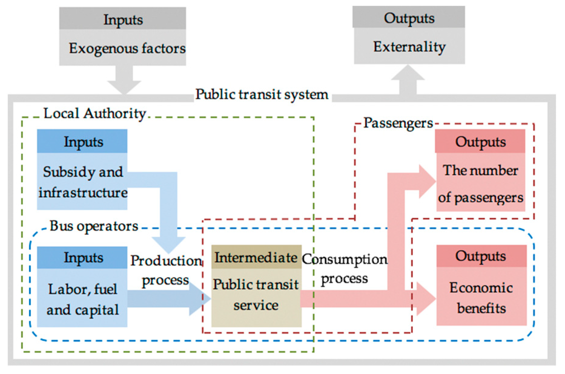
The DEA, which is introduced by Farrell [31] and popularized by Charnes et al. [32], is an analytical method that uses a linear programming technique to evaluate the relative performance of decision-making units (DMUs). This method for evaluating public transit system is constantly ongoing and affluent. This affluence mainly arises from multiple perspectives and diverse measurement models. As discussed in Zhao et al. [14], the operation of public transit involves three stakeholders, namely, bus operators, passengers, and local authority. Different stakeholders are concerned about different issues, so different measurement perspectives can be obtained when considering different stakeholders. More concretely, bus operators strive to minimize the operating inputs and maximize their economic benefits and, thus, production efficiency is proposed to evaluate the service provision capacity of bus operators by using production-oriented variables (e.g., vehicle-km or seat-km) [33]. 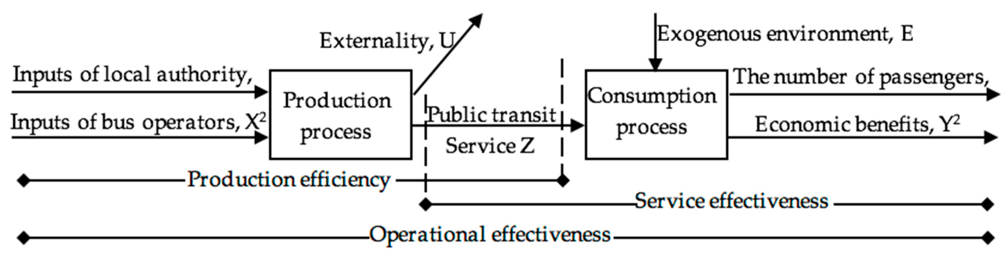Passengers expect superior public transit service to meet their daily travel requirements and, accordingly, service effectiveness is proposed to evaluate the service consumption capacity of passengers by employing service-oriented variables (e.g., passengers or passenger-km) [27,34]. Governments focus on both their own financial investments and the whole public transit system, so operational effectiveness is proposed to evaluate the performance of public transit system by combining production efficiency and service effectiveness [35,36,37] or by adding government input variables (e.g., the amount of subsidy) [38,39]. In addition to three stakeholders within the public transit system, some researchers expanded public transit performance measurement to a broader perspective. For example, Yu and Fan [15], and Karlaftis and Tsamboulas [40] considered uncontrollable environmental factors (e.g., population density, car ownership, and area) in the measurement model in order to eliminate the effects of the operating environment on the performance of public transit. Kang et al. [13] found that bus transit firms’ technical efficiency was affected by their environmental pollution. These studies showed that the performance of public transit was impacted by the exogenous environment. However, none of the abovementioned literature has taken all perspectives (i.e., local authority, bus operators, passengers, uncontrollable environmental factors, and the externality of public transit) into account. Therefore, it is necessary to integrate all perspectives to measure the performance of the public transit system at the city level.

The multiple perspectives and settings have derived kinds of measurement models. Some papers used the original CCR (Charnes-Cooper-Rhodes) and BCC (Banker-Charnes-Cooper) that respectively assume constant return to scale (CRS) and variable return to scale (VRS) to measure public transit performance [25,40], but most papers paid more attention to improving the measurement approach by modifying DEA or combining DEA with other models. For example, given that transit firms may generate both desirable and undesirable outputs while some of which may only take integer values, Chen et al. [18] proposed an integer DEA model with undesirable inputs and outputs. Boame [26] used a bootstrap DEA to estimate technical efficiency for Canadian transit systems from 1990 to 1998. The bootstrap method may estimate bias and confidence intervals for the efficiency scores in order to assess their precision. Zhang et al. [39] combined the information entropy theory and super-efficiency DEA to evaluate 13 transit operators in Yangtze Delta of China. All model improvements were aimed at enhancing measurement models’ applicability and discrimination capability. Nevertheless, existing studies ignored the consideration of measurement variables with boundary values, such as passenger satisfaction. This neglect may overestimate the efficiency score for output-oriented models. Furthermore, an important purpose of public transit performance measurement is to find operational deficiencies and propose feasible projections to improve the performance of inefficient transit systems, but only a few studies have carried out efficiency frontier analysis [16,41].

In a nutshell, most previous studies evaluating the public transit system have considered one or just a few perspectives, and have not included all the perspectives thought to influence public transit system evaluation. Second, it cannot be ignored that the measurement variables with boundary values may lead to overestimating of the efficiency score, and no studies have addressed this issue. Third, inefficient public transit systems have rarely been further investigated. These considerations represent significant gaps in the literature. Therefore, this study attempts to address these gaps found in previous research by (1) integrating all relevant perspectives into the public transit system evaluation, namely, local authority, bus operators, passengers, uncontrollable environmental factors, and the externality of public transit; (2) constructing a measurement model by simultaneously considering boundary-valued variables, uncontrollable environmental factors, and undesirable outputs; and (3) projecting inefficient transit systems to efficiency in a case study.

3. Research Design

3.1. Measurement Framework

The measurement framework in our study mainly expands on several major existing studies. First, public transit system operation is a complex process involving multiple stakeholders, i.e., bus operators, passengers, and local authority [14]. These three stakeholders participate in the public transit system in different ways. For example, from the bus operators’ point of view, they input labor, fuel, and capital to produce public transit service, and obtain economic benefits after the process of passengers’ consumption. From the passengers’ perspective, they consume the public transit service to meet their daily travel requirements. From the local authority’s point of view, they decide whether or not to expand or abolish the transit infrastructure [22]. Moreover, they may provide financial subsidies to bus operators to ensure the regular production of transit service. The subsidy and investment are involved as local authority’s input in the production process.

Second, it is worth noting that the exogenous environment in which the public transit system operated may impact the performance of the transit system. For example, population or population density are positively correlated with transit ridership, while car ownership has a negative impact [42,43,44]. According to Banker and Morey [45], the comparison among DMUs should be conducted in a similar or harsher environment. On the other hand, the public transit system, in turn, may have feedback or externality to the exogenous environment, such as accidents, emissions, and others. The externality of public transit also has a significant influence on the performance evaluation [13]. Therefore, measuring the performance of the public transit system should not only investigate the underlying structure of three different stakeholders in the public transit system but also pay attention to the interaction between the public transit system and its exogenous environment. Figure 1 presents the structure of a public transit system with respect to the three perspectives and its interaction with the exogenous urban environment.

Finally, unlike ordinary manufacturing enterprises’ production and consumption process, the consumption process of public transit service occurs simultaneously with the production process. More concretely, the public transit service cannot be stored. Once the public transit service is produced, it ceases to exist regardless of whether it was consumed [35]. Therefore, it is quite essential to identify the fact that only a portion of transit service is consumed in general. The consumed service may differ greatly from the produced service. To solve this issue, Yu and Fan [15] proposed production efficiency, service effectiveness, and operational effectiveness to measure the public transit system’s production performance, consumption performance, and overall operational performance, respectively. Note that the operational effectiveness is obtained by combining production efficiency and service effectiveness.

To sum up, according to Zhao et al. [14], the operation of public transit involves three stakeholders, i.e., the local authority provides investment and financial support to the public transit system, bus operators produce the public transit service, and passengers then consume the public transit service. According to Yu and Fan [15] and Karlaftis and Tsamboulas [40], in order to eliminate the effects of the operating environment on the performance of public transit, it is necessary to incorporate uncontrollable environmental factors into the measurement model. According to Kang et al. [13], the feedback from public transit to exogenous environment, namely, externality, also has a significant impact on the performance measurement. Therefore, we take all perspectives (i.e., local authority, bus operators, passengers, uncontrollable environmental factors. and the externality of public transit) into account. Consistent with the discussion above, our measurement framework contains five parts, i.e., inputs (the local authority’s inputs X¹, the bus operators’ inputs X²), the intermediate outputs (public transit service Z), outputs (the number of passengers Y¹, bus operators’ economic benefits Y²), uncontrollable environmental factors E, and the externality of public transit system U. Meanwhile, the measurement framework can simultaneously capture each public transit system’s production efficiency, service effectiveness, and operational effectiveness. Finally, the measurement framework of the public transit system is shown in Figure 2.

3.2. Methodology

3.2.1. SE-NDEA Model

Due to the network structure of the above measurement framework, we adopt the network DEA method, proposed by Färe and Grosskopf [46], as the fundamental model in this paper. Meanwhile, given that the advantage of super-efficiency DEA for ranking efficient DMUs further by excluding the DMU itself from the sample set [47], we combine these two models and generate super-efficiency network DEA (SE-NDEA). Moreover, there may be zero inputs in the measurement, for example, governments do not always provide subsidies to bus operators, so we choose an output-oriented model.

Assume that there are N DMUs and the jth DMU (j = 1, 2, …, N) uses input quantities X_j = {X¹_j, X²_j} to produce intermediate output quantities Z_j and final output quantities Y_j = {Y¹_j, Y²_j}. We also assume that X = (x_ij)∈R^M×N, Z = (z_rj)∈R^S×N and Y = (y_oj)∈R^L×N are non-negative. Then, the output-oriented SE-NDEA model can be described as

$${\mathrm{D}}_{SE-NDEA}\{\begin{array}{c}max\left(w_1{\beta }_1+w_2{\beta }_2\right)\\ {\displaystyle \sum _{j=1,j\ne j_0}^n}{X}_j{\lambda }_j^1\le X_{j_0}\\ {\displaystyle \sum _{j=1,j\ne j_0}^n}{Z}_j{\lambda }_j^1\ge {\beta }_1{Z}_{j_0}\\ {\displaystyle \sum _{j=1,j\ne j_0}^n}{Z}_j{\lambda }_j^2\le {\beta }_1{Z}_{j_0}\\ {\displaystyle \sum _{j=1,j\ne j_0}^n}{Y}_j{\lambda }_j^2\ge {\beta }_2{Y}_{j_0}\\ {\lambda }_j^1,{\lambda }_j^2\ge 0,j=1,2,\dots ,N\end{array}$$

(1)

where β₁ and β₂ denote the optimal efficiency score of the production process and consumption process, namely, production efficiency and service effectiveness, respectively. If β₁ ≤ 1, this indicates the DMU is production-efficient. Otherwise, it is production-inefficient. Similarly, if β₂ ≤ 1, this indicates the DMU is service-effective, otherwise, it is service-ineffective. Note that the larger the β, the lower the efficiency. λ¹ and λ² are positive intensity variables related to the production process and consumption process. w₁ and w₂ are weight coefficients to define the relative importance of the two processes and, thus, w₁ + w₂ = 1.

3.2.2. SE-NDEA Model with Undesirable Outputs

The SE-NDEA presented above assumes that all inputs and outputs are desirable, and means that the more inputs, the more outputs, and more is always preferred to less [18]. However, the performance measurement of the public transit system does not always abide by this assumption, due to different measurement contents. For example, the outputs from public transit system operation may include the number of accidents, noise pollution, and CO₂ emissions, all of which are undesirable [12]. To solve this issue, some other studies have introduced undesirable outputs by using their reciprocals or opposite number to transform negative outputs into positive ones [38,48,49]. Nevertheless, according to Liu and Sharp [50], the numerical transformation may distort the results, i.e., the evaluation reference and the ranking results may depend on the transformation approach adopted. Thus, in this paper, we use a more general and simpler alternative method proposed by Berg et al. [51], i.e., treating the undesirable outputs as inputs, namely [INP]. The inequalities for dealing with undesirable outputs are given by

$${\displaystyle \sum }_{j=1,j\ne j_0}^n{Z}^U{}_j{\lambda }_j^1\le Z^U{}_{j_0}$$

(2)

$${\displaystyle \sum }_{j=1,j\ne j_0}^n{Y}^U{}_j{\lambda }_j^2\le Y^U{}_{j_0}$$

(3)

where Z^U and Y^U are the quantities of undesirable intermediate outputs and undesirable final outputs, respectively. If there are undesirable intermediate outputs in the process of production, we use an inequality constraint (2) to compare the production efficiency by maintaining the undesirable intermediate outputs of the j₀th DMU as no less than those of the samples. Based on the same idea, if there are undesirable final outputs in the consumption process, the inequality constraint (3) is used to compare the service effectiveness.

3.2.3. SE-NDEA Model with Uncontrollable Constraints

As discussed in Section 3.1, uncontrollable environmental factors may have a significant impact on the performance of public transit systems, such as population and car ownership [43]. Therefore, in order to overcome limitations, we consider the exogenous factors by imposing constraints on the consumption activity as follows:

$${\displaystyle \sum }_{j=1,j\ne j_0}^n{E}^P{}_j{\lambda }_j^2\le E^P{}_{j_0}$$

(4)

$${\displaystyle \sum }_{j=1,j\ne j_0}^n{E}^N{}_j{\lambda }_j^2\ge E^N{}_{j_0}$$

(5)

where E^P and E^N are the quantity of two types of exogenous factors. According to Yu and Fan [15], if exogenous factors have a positive correlation with the service effectiveness, we can compare a public transit system’s service effectiveness in the case of keeping the exogenous factors equal to or better than the circumstance they face by employing the inequality constraint (4). On the contrary, if exogenous factors have a negative influence on the service effectiveness, an inequality constraint (5) can be adopted to maximize the potential increase of the final outputs (e.g., the number of passengers) for public transit system j₀ while keeping the exogenous factors no better than the current circumstance it faces.

3.2.4. SE-NDEA Model with Boundary-Valued Variables

It is worth noting that one may select ratio variables to measure the performance of public transit, such as the error rate of average headway and passenger satisfaction [11,39]. However, previous studies do not consider the presence of boundary on these ratio variables. This neglect may overestimate the efficiency score for output-oriented models and result in misleading improvement projections which should have contributed to efficiency. To solve this issue, we introduce additional constraints to Model (1) by taking the following forms:

$${\displaystyle \sum }_{j=1,j\ne j_0}^n{Z}^B{}_j{\lambda }_j^1\le 100$$

(6)

$${\displaystyle \sum }_{j=1,j\ne j_0}^n{Y}^B{}_j{\lambda }_j^2\le 100$$

(7)

where Z^B and Y^B are the quantities of boundary-valued intermediate outputs and boundary-valued final outputs, respectively. In the process of production, we apply an inequality constraint (6) to ensure intermediate outputs with a ratio value of the j₀th DMU no more than 100, and the inequality constraint (7) applies to the consumption process.

Ultimately, we develop the final SE-NDEA model as follows. We use Z^D, Z^U, Z^B, Y^D, Y^U, and Y^B to respectively represent desirable intermediate outputs, undesirable intermediate outputs, boundary-valued intermediate outputs, desirable final outputs, undesirable final outputs, and boundary-valued final outputs, where Z^D covers Z^B and Y^D covers Y^B. It can be seen that constraints (8)–(11) are the constraints of the original SE-NDEA model represented in Section 3.2.1, and constraints (12)–(17) are added on the basis of the original model. Specifically, Constraint (8) is used for local authority and bus operators’ inputs. Constraints (9) and (10) are applicable for desirable intermediate outputs, such as vehicle kilometers. Constraint (11) applies to desirable final outputs, such as ridership. Constraints (12) and (13) are used for undesirable outputs. More concretely, Constraint (12) applies to undesirable intermediate outputs, such as CO₂ emissions, death tolls, and Constraint (13) applies to undesirable final outputs, such as passenger complaints. Constraints (14) and (15) are used for boundary-valued outputs. Among them, Constraint (14) is applicable for boundary-valued intermediate outputs, such as punctuality, and Constraint (15) is applicable for boundary-valued final outputs, such as passenger satisfaction. Constraints (16) and (17) are adopted to eliminate the impacts of uncontrollable environmental factors. Furthermore, Constraint (16) is applicable for exogenous factors that have a positive correlation with public transit system patronage, such as urban population, whereas Constraint (17) is applicable for exogenous factors that have a negative correlation, such as car ownership.

It should be noted that the network DEA and super-efficiency DEA are both linear programs [46,47], and the constraints we added are a series of linear inequality constraints, familiar from DEA. Therefore, the following SE-NDEA model is also a linear program. The added constraints do not increase the complexity of the model solving. Regarding the linear programming problem, the software of MATLAB (R2018b, The MathWorks, Inc., US) is a powerful tool due to its ready-made linear programming solver. Thus, in this paper, we adopted the R2018b version of MATLAB to solve this model.

$$max\left(w_1{\beta }_1+w_2{\beta }_2\right),s.t:{{\displaystyle \sum }}_{j=1,j\ne j_0}^n{X}_j{\lambda }_j^1\le X_{j_0}$$

(8)

$${\displaystyle \sum }_{j=1,j\ne j_0}^n{Z}^D{}_j{\lambda }_j^1\ge {\beta }_1{Z}^D{}_{j_0}$$

(9)

$${\displaystyle \sum }_{j=1,j\ne j_0}^n{Z}^D{}_j{\lambda }_j^2\le {\beta }_1{Z}^D{}_{j_0}$$

(10)

$${\displaystyle \sum }_{j=1,j\ne j_0}^n{Y}^D{}_j{\lambda }_j^2\ge {\beta }_2{Y}^D{}_{j_0}$$

(11)

$${\displaystyle \sum }_{j=1,j\ne j_0}^n{Z}^U{}_j{\lambda }_j^1\le Z^U{}_{j_0}$$

(12)

$${\displaystyle \sum }_{j=1,j\ne j_0}^n{Y}^U{}_j{\lambda }_j^2\le Y^U{}_{j_0}$$

(13)

$${\displaystyle \sum }_{j=1,j\ne j_0}^n{Z}^B{}_j{\lambda }_j^1\le 100$$

(14)

$${\displaystyle \sum }_{j=1,j\ne j_0}^n{Y}^B{}_j{\lambda }_j^2\le 100$$

(15)

$${\displaystyle \sum }_{j=1,j\ne j_0}^n{E}^P{}_j{\lambda }_j^2\le E^P{}_{j_0}$$

(16)

$${\displaystyle \sum }_{j=1,j\ne j_0}^n{E}^N{}_j{\lambda }_j^2\ge E^N{}_{j_0}$$

(17)

$${\lambda }_j^1,{\lambda }_j^2\ge 0,j=1,2,\dots ,N$$

(18)

Finally, in order to be consistent with previous literature, i.e., the larger the efficiency score, the higher the efficiency, we introduced the reciprocal of β, namely, θ₁ = 1/β₁ and θ₂ = 1/β₂, to respectively measure the production efficiency and service effectiveness. Moreover, in this paper, we considered the production process to be as important as the consumption process, so we set w₁ = w₂ = 0.5, then the overall performance of public transit system, i.e., operational effectiveness, is 0.5θ₁ + 0.5θ₂.

3.3. Variables Selection

We should not ignore the fact that the DEA scores are highly sensitive to the selection of input and output variables [37]. Therefore, for the purpose of measuring the performance of the public transit system more accurately and realistically, we selected inputs and outputs variables based on the following principles: (a) the acceptance by the national and local department in charge of public transit, (b) the application in previous studies, and (c) the availability of practitioners and researchers.

Regarding input variables of the local authority, the length of bus lines and subsidies have often been used in previous literature [22,38,39]. Moreover, the bus prior line is a major measure for governments to improve transit service (e.g., bus speed), so we used the length of bus prior lines as the third input variable of the local authority. Regarding input variables of bus operators, we select employees and vehicles to measure bus operators’ labor and capital. Regarding intermediate output variables related to transit service, the conventional variable used in the previous network DEA is vehicle kilometers [15,52]. However, vehicle-km only measures the quantity of public transit service and does not consider the quality of the transit service. Thus, in addition to vehicle-km, we also adopt average speed and punctuality to measure the public transit service quality. Regarding output variables, bus ticket revenue and annual ridership respectively represent the bus operators’ economic benefits and the number of passengers. In addition, from the passengers’ perspective, ridership represents the passengers’ objective behavior, so we concurrently capture passenger satisfaction as another final output for measuring the passengers’ subjective perception [53]. Note that the punctuality and passenger satisfaction are both variables with boundary values. Regarding externality variables, because public transit has the positive externality of reducing traffic accidents, we choose the death toll for measuring the feedback of the public transit system on the external environment. This externality variable needs to be minimized. At last, regarding uncontrollable environmental variables, population and car ownership were considered, referring to earlier literature [42,43,44]. All descriptions and sources of variables used in this paper are shown in

Table 1. Variables used in the super efficiency network data envelopment analysis (SE-NDEA) model.

Variables	Description	Sources
Subsidies (million RMB), X1	Total annual government subsidies	Municipal Bureau of Finance
Bus lines length (km), X2	The length of operating bus lines	Local Statistical Yearbook
Bus prior lines length (km), X3	The length of operating bus prior lines	Local Statistical Yearbook
Employees (one), X4	The number of employed workers	Municipal Transport Commission
Vehicles (one), X5	The number of vehicles in operation	Local Statistical Yearbook
Vehicle-km (10,000 km), ZD1	Total annual operating kilometers	Local Statistical Yearbook
Speed (km/h), ZD2	Average speed in peak hours	Municipal Transport Commission
Punctuality (%), ZB	The ratio of punctual trips to all trips	Municipal Transport Commission
Revenue (10,000 RMB), YD1	Annual bus ticket revenue	Municipal Transport Commission
Ridership (10,000), YD2	Annual ridership	Local Statistical Yearbook
Passenger satisfaction (%), YB	Average score of specified questionnaires	Municipal Transport Commission
Death toll (one), ZU1	The number of traffic accidents	Municipal Transport Commission
Population (10,000), EP	The number of habitual residents	Local Statistical Yearbook
Car ownership (10,000), EN	The number of private cars	Local Statistical Yearbook

.

4. Empirical Study

4.1. Data

In this study, the unit of analysis is the public transit system. Thus, annual data at the city level are used. Although bus priority policy was put forward in China in 2004, most cities have not been implemented until 2008. Therefore, we will perform an empirical study with the data corresponding to an eight-year period, from 2009 to 2016. Measure the performance of the public transit system in this period is meaningful for China.

We collected a set of empirical data from 11 Chinese cities: Shenzhen, Guangzhou, Shijiazhuang, Suzhou, Jinan, Hangzhou, Hefei, Taiyuan, Urumqi, Haikou, and Yinchuan. These are all exemplary cities of transit metropolis construction in China. Their public transit performance is representative to a certain extent. According to the “Notice on Adjusting the Standard of Urban Size” proposed by China’s State Council in 2014, these cities are divided into three categories based on the populations of habitual residents, as shown in

Table 2. Decision-making units (DMUs).

Urban Size	Population	City Name
Super city	Equal to or more than ten million	Shenzhen, Guangzhou, Shijiazhuang, Suzhou
Mega city	Between five million and ten million	Jinan, Hangzhou, Hefei
Large city	Between one million and five million	Taiyuan, Urumqi, Haikou, Yinchuan

. One year in each city is considered as a DMU.

Table 3. Descriptive statistics.

Variables	Max	Median	Min	Mean	Std. Deviation
Subsidies, X1	5190	260.64	26.91	993.62	1425.27
Bus lines length, X2	21462.2	4122.5	420	6526.81	6223.72
Bus prior lines length, X3	957	79.5	10	142.05	199.92
Employees, X4	68562	12505	6730	19111.49	15883.39
Vehicles, X5	17075	5100	1346	6625.23	4740.71
Vehicle-km, ZD1	130450.6	19627.34	5792.67	34425.06	35365.93
Speed, ZD2	99.25	71.79	50.6	73.44	11.34
Punctuality, ZB	32.71	20.07	10	21.09	5.09
Revenue, YD1	871151	82254	13381.06	193245.38	245771.75
Ridership, YD2	495646	73116	17378	122485.03	124229.47
Satisfaction, YB	94.02	76.68	65.5	77.9	6.77
Death toll, ZU1	27	7	2	8.36	4.75
Population, EP	1404.35	759	187.85	721.12	367.85
Car ownership, EN	277.58	63.46	11.42	86.47	66.56

provides the variables’ descriptive statistics for the dataset.

4.2. Results

4.2.1. Performance Review

After running the SE-NDEA model using the software of MATLAB, we obtain 11 cities’ production efficiency, service effectiveness, and operational effectiveness from 2009 to 2016. All scores are presented in

Table A1. Production efficiency.

Urban Size	DMUs	Period								Mean
		2009	2010	2011	2012	2013	2014	2015	2016
Super city	Shenzhen	0.96	1.05	0.96	1.07	0.97	0.93	0.95	1.19	1.01
	Guangzhou	1.18	1.05	1.11	1.04	1.01	1.03	1.00	1.05	1.06
	Shijiazhuang	0.76	0.79	0.77	0.79	0.77	0.75	0.73	0.75	0.76
	Suzhou	1.00	1.00	1.00	1.00	1.03	1.01	1.02	1.02	1.01
	Mean	0.98	0.97	0.96	0.98	0.95	0.93	0.93	1.00	0.96
Mega city	Jinan	0.82	0.74	0.69	0.67	0.68	0.69	0.74	0.81	0.73
	Hangzhou	0.71	0.73	0.73	0.86	0.87	0.96	0.93	0.97	0.85
	Hefei	0.73	0.73	0.72	0.73	0.73	0.75	0.74	0.72	0.73
	Mean	0.75	0.73	0.71	0.75	0.76	0.80	0.80	0.83	0.77
Large city	Taiyuan	0.62	0.63	0.58	0.59	0.60	0.60	0.61	0.60	0.60
	Urumqi	0.71	0.71	0.72	0.72	0.73	0.73	0.73	0.74	0.72
	Haikou	0.74	0.74	0.74	0.74	0.74	0.74	0.74	0.75	0.74
	Yinchuan	0.68	0.69	0.69	0.70	0.70	0.70	0.71	0.71	0.70
	Mean	0.69	0.69	0.68	0.69	0.69	0.69	0.70	0.70	0.69

,

Table A2. Service effectiveness.

Urban Size	DMUs	Period								Mean
		2009	2010	2011	2012	2013	2014	2015	2016
Super city	Shenzhen	0.84	0.89	0.88	0.98	0.98	1.00	0.94	1.25	0.97
	Guangzhou	1.01	1.03	1.14	1.03	1.01	1.05	1.00	1.03	1.04
	Shijiazhuang	0.68	0.69	0.70	0.70	0.71	0.71	0.71	0.72	0.70
	Suzhou	0.71	0.71	0.72	0.77	0.78	0.80	0.84	1.29	0.83
	Mean	0.81	0.83	0.86	0.87	0.87	0.89	0.87	1.07	0.88
Mega city	Jinan	0.93	0.93	0.93	0.93	0.94	0.94	0.94	0.94	0.94
	Hangzhou	0.86	0.89	0.86	0.78	0.79	0.86	0.89	0.87	0.85
	Hefei	0.73	0.75	0.75	0.76	0.76	0.77	0.78	0.80	0.76
	Mean	0.84	0.86	0.85	0.82	0.83	0.86	0.87	0.87	0.85
Large city	Taiyuan	0.66	0.67	0.69	0.70	0.70	0.71	0.71	0.72	0.70
	Urumqi	0.90	0.89	0.87	0.87	1.00	0.98	0.97	1.00	0.94
	Haikou	1.00	0.97	0.94	0.94	0.93	0.92	0.89	0.91	0.94
	Yinchuan	1.00	0.96	0.98	1.00	1.00	0.99	0.99	1.00	0.99
	Mean	0.89	0.87	0.87	0.88	0.91	0.90	0.89	0.91	0.89

and

Table A3. Operational effectiveness.

Urban Size	DMUs	Period								Mean
		2009	2010	2011	2012	2013	2014	2015	2016
Super city	Shenzhen	0.90	0.97	0.92	1.03	0.98	0.97	0.95	1.22	0.99
	Guangzhou	1.10	1.04	1.13	1.04	1.01	1.04	1.00	1.04	1.05
	Shijiazhuang	0.72	0.74	0.74	0.75	0.74	0.73	0.72	0.74	0.74
	Suzhou	0.86	0.86	0.86	0.89	0.91	0.91	0.93	1.16	0.92
	Mean	0.90	0.90	0.91	0.93	0.91	0.91	0.90	1.04	0.93
Mega city	Jinan	0.88	0.84	0.81	0.80	0.81	0.82	0.84	0.88	0.84
	Hangzhou	0.79	0.81	0.80	0.82	0.83	0.91	0.91	0.92	0.85
	Hefei	0.73	0.74	0.74	0.75	0.75	0.76	0.76	0.76	0.75
	Mean	0.80	0.80	0.78	0.79	0.80	0.83	0.84	0.85	0.81
Large city	Taiyuan	0.64	0.65	0.64	0.65	0.65	0.66	0.66	0.66	0.65
	Urumqi	0.81	0.80	0.80	0.80	0.87	0.86	0.85	0.87	0.83
	Haikou	0.87	0.86	0.84	0.84	0.84	0.83	0.82	0.83	0.84
	Yinchuan	0.84	0.83	0.84	0.85	0.85	0.85	0.85	0.86	0.85
	Mean	0.79	0.79	0.78	0.79	0.80	0.80	0.80	0.81	0.80

in the Appendix A. Note that if the score of efficiency or effectiveness is equal to or greater than unity, it is considered “efficient”. If the score is between 0.8 (inclusive) and 1, it is “fairly efficient”. If the score is less than 0.8, it is “inefficient”.

Table 4. The average efficiency and effectiveness score for all DMUs.

Urban Size	DMUs	Production Efficiency		Service Effectiveness		Operational Effectiveness
		Score	Rank	Score	Rank	Score	Rank
Super city	Shenzhen	1.01	2	0.97	3	0.99	2
	Guangzhou	1.06	1	1.04	1	1.05	1
	Shijiazhuang	0.76	5	0.7	10	0.74	10
	Suzhou	1.01	2	0.83	8	0.92	3
	Mean	0.96	I	0.89	II	0.93	I
Mega city	Jinan	0.73	6	0.94	4	0.84	6
	Hangzhou	0.85	4	0.85	7	0.85	4
	Hefei	0.73	6	0.76	9	0.75	9
	Mean	0.77	II	0.85	III	0.81	II
Large city	Taiyuan	0.6	11	0.70	10	0.65	11
	Urumqi	0.72	9	0.93	5	0.83	8
	Haikou	0.74	8	0.93	5	0.84	6
	Yinchuan	0.70	10	0.99	2	0.85	4
	Mean	0.69	III	0.89	I	0.79	III

summarizes the overall performance results of all cities and their ranking order. It is worth noting that the overall performance of a city is calculated by the average score from 2009 to 2016.

As can be seen, these operational effectiveness scores are between 0.65 and 1.05. This shows that there are great differences in the public transit operation among cities. There was only one city whose public transit operation was considered effective—Guangzhou. Moreover, Guangzhou was also the only city that achieved efficient production and effective service at the same time. Meanwhile, nearly two-thirds of cities have a fairly effective public transit system. They are Shenzhen, Suzhou, Hangzhou, Yinchuan, Jinan, Haikou, and Urumqi. Finally, public transit operation in Hefei, Shijiazhuang, and Taiyuan were ineffective. Taiyuan, in particular, had the worst public transit performance among all cities. This is due to the fact that Taiyuan’s outputs are insufficient compared with other cities. For example, the passenger satisfaction of Taiyuan is relatively low according to its operational data.

From the overall perspective, super cities tended to perform better than mega cities, and mega cities tended to perform better than large cities. It is interesting to find that some cities tend to perform well on one measure and perform badly on the other. For example, Yinchuan has relatively high service effectiveness (0.99) and low production efficiency (0.70). Further, Figure 3 presents the service effectiveness versus production efficiency of all DMUs. For super cities, the service effectiveness was generally lower than the production efficiency, whereas, for large and mega cities, the service effectiveness was generally higher. These results suggest that, for a number of exogenous and operational reasons, a city with a large population is more likely to be production-efficient than service-effective.

The above conclusion raises the question: How are production efficiency and service effectiveness related? Using the scores of production efficiency and service effectiveness of all DMUs, the correlation coefficient between the two variables was calculated. The value of Pearson correlation is 0.386, and the p-value equal to 0.000 is smaller than 0.05 (2-tailed). This implies that service effectiveness has a significantly positive correlation with production efficiency, i.e., a city that performs well in production process tends to also perform well in consumption process. This is consistent with the findings by Karlaftis [35].

From the time dimension, Figure 4 shows the operational effectiveness trends from 2009 to 2016. In particular, the proportion of operational effectiveness less than 0.7 remains constant (9.09%), and the operational effectiveness between 0.7 (inclusive) and 0.9 decreased by 18.18%, and the corresponding operational effectiveness which is equal to or greater than 0.9 increased by 18.18%. Clearly, there has been a steady increase in the performance of public transit system. This indicates that the bus priority policy has had a positive effect in China.

In addition, compared to conventional bus, transit rail has the advantage of large capacity, high speed, greater punctuality and energy saving, and is gradually shouldering the backbone of urban public transit systems. Hence, an important question needs to be answered: Is transit rail’s operational effectiveness higher than that of conventional bus? Figure 5 exhibits a comparison between the two modes in the four cities that have put transit rail into operation. The figure clearly reveals that transit rail has surely more operational effectiveness than conventional bus. However, even with this superiority, the transit rail does not always have the ability to improve the operational effectiveness of the whole public transit system. For example, Suzhou’s average operational effectiveness of the whole system is equal to that of conventional bus (0.92). This implies that Suzhou’s operational effectiveness has not improved since the transit rail opened. Hangzhou’s operational effectiveness has even descended (0.89 to 0.85). It is remarkable that Shenzhen and Guangzhou have respectively put eight and nine rail lines into operation by the time of this study, and Suzhou and Hangzhou have opened two and three lines, respectively. We infer that the transit rail network scale in a city may determine whether the transit rail has a positive effect on the overall operational effectiveness of the urban public transit systems. That is to say, in a city with a large-scale transit rail, the transit rail may improve the city’s overall operational effectiveness; otherwise, this is not the case.

4.2.2. Exogenous Environment Analysis

To eliminate the impact of exogenous environment on the performance of the public transit system, we integrated uncontrollable environmental factors and the externality of public transit into the measurement framework. However, any differences resulting from introduction of these two types of environmental variables has not yet investigated. Therefore, based on the panel data of 11 cities from 2009 to 2016, we further calculated other operational effectiveness scores without considering environmental variables, as shown in

Table A4. Production efficiency.

Urban Size	DMUs	Period								Mean
		2009	2010	2011	2012	2013	2014	2015	2016
Super city	Shenzhen	0.78	0.93	0.90	1.01	0.93	0.90	0.90	0.98	0.92
	Guangzhou	0.98	1.00	1.04	1.00	0.95	0.94	0.94	0.98	0.98
	Shijiazhuang	0.76	0.79	0.77	0.76	0.74	0.72	0.71	0.71	0.75
	Suzhou	1.00	0.99	0.98	0.95	0.97	0.99	0.99	0.99	0.98
	Mean	0.88	0.93	0.92	0.93	0.90	0.89	0.89	0.92	0.91
Mega city	Jinan	0.82	0.74	0.69	0.67	0.68	0.68	0.69	0.70	0.71
	Hangzhou	0.71	0.72	0.73	0.86	0.87	0.84	0.93	0.93	0.82
	Hefei	0.68	0.68	0.69	0.69	0.70	0.71	0.71	0.72	0.70
	Mean	0.74	0.71	0.70	0.74	0.75	0.74	0.78	0.78	0.74
Large city	Taiyuan	0.62	0.63	0.52	0.52	0.54	0.54	0.55	0.55	0.56
	Urumqi	0.71	0.72	0.72	0.72	0.73	0.73	0.73	0.74	0.73
	Haikou	0.72	0.73	0.73	0.73	0.74	0.74	0.74	0.75	0.74
	Yinchuan	0.68	0.69	0.69	0.70	0.70	0.70	0.71	0.71	0.70
	Mean	0.68	0.69	0.67	0.67	0.68	0.68	0.68	0.69	0.68

,

Table A5. Service effectiveness.

Urban Size	DMUs	Period								Mean
		2009	2010	2011	2012	2013	2014	2015	2016
Super city	Shenzhen	0.77	0.79	0.80	0.87	0.88	0.87	0.84	0.86	0.84
	Guangzhou	0.84	0.98	1.04	0.99	0.95	0.94	0.94	0.95	0.95
	Shijiazhuang	0.68	0.69	0.70	0.70	0.71	0.71	0.71	0.72	0.70
	Suzhou	0.71	0.71	0.72	0.77	0.78	0.80	0.81	0.82	0.77
	Mean	0.75	0.79	0.82	0.83	0.83	0.83	0.83	0.84	0.82
Mega city	Jinan	0.93	0.93	0.93	0.93	0.94	0.94	0.94	0.94	0.94
	Hangzhou	0.74	0.74	0.74	0.78	0.79	0.80	0.80	0.85	0.78
	Hefei	0.73	0.75	0.75	0.76	0.76	0.77	0.78	0.80	0.76
	Mean	0.80	0.81	0.81	0.82	0.83	0.84	0.84	0.86	0.83
Large city	Taiyuan	0.65	0.66	0.69	0.70	0.70	0.71	0.71	0.72	0.69
	Urumqi	0.72	0.73	0.74	0.75	0.75	0.75	0.75	0.76	0.74
	Haikou	0.73	0.73	0.74	0.75	0.76	0.76	0.75	0.76	0.75
	Yinchuan	0.80	0.81	0.82	0.83	0.83	0.84	0.83	0.84	0.83
	Mean	0.73	0.73	0.75	0.76	0.76	0.77	0.76	0.77	0.75

and

Table A6. Operational effectiveness.

Urban Size	DMUs	Period								Mean
		2009	2010	2011	2012	2013	2014	2015	2016
Super city	Shenzhen	0.78	0.86	0.85	0.94	0.91	0.89	0.87	0.92	0.88
	Guangzhou	0.91	0.99	1.04	1.00	0.95	0.94	0.94	0.97	0.97
	Shijiazhuang	0.72	0.74	0.74	0.73	0.73	0.72	0.71	0.72	0.73
	Suzhou	0.86	0.85	0.85	0.86	0.88	0.90	0.90	0.91	0.88
	Mean	0.82	0.86	0.87	0.88	0.87	0.86	0.86	0.88	0.87
Mega city	Jinan	0.88	0.84	0.81	0.80	0.81	0.81	0.82	0.82	0.82
	Hangzhou	0.73	0.73	0.74	0.82	0.83	0.82	0.87	0.89	0.80
	Hefei	0.71	0.72	0.72	0.73	0.73	0.74	0.75	0.76	0.73
	Mean	0.77	0.76	0.76	0.78	0.79	0.79	0.81	0.82	0.78
Large city	Taiyuan	0.64	0.65	0.61	0.61	0.62	0.63	0.63	0.64	0.63
	Urumqi	0.72	0.73	0.73	0.74	0.74	0.74	0.74	0.75	0.74
	Haikou	0.73	0.73	0.74	0.74	0.75	0.75	0.75	0.76	0.74
	Yinchuan	0.74	0.75	0.76	0.77	0.77	0.77	0.77	0.78	0.76
	Mean	0.71	0.72	0.71	0.72	0.72	0.72	0.72	0.73	0.72

in Appendix B. Furthermore, to test whether the two operational effectiveness scores are significantly different, i.e., Table A3 vs. Table A6, we conducted a nonparametric test (the Mann-Whitney U test). The Z value of the test is −3.372, and the p-value equal to 0.001 is smaller than 0.05 (2-tailed). Thus, we reject the null hypothesis at a significance level of 0.05, suggesting that the operational effectiveness under the two considerations are significantly different. The exogenous environment has a marked impact on the performance measurement for the public transit system.

4.2.3. Projecting to Efficiency

An important objective of performance evaluation of the public transit system is to identify the deficiency in inefficient systems and propose feasible measures to improve their performance. Specifically, each inefficient DMU needs to be projected onto the efficiency frontier derived from the SE-NDEA model either by (a) decreasing the current level of inputs while maintaining outputs, or (b) increasing outputs while maintaining the inputs [18]. Regarding public transit, because of the great support by central and local governments due to its positive externalities, strategies that involve decreasing inputs are always inapplicable. Thus, we chose strategies addressing (b) as our primary measures. That is also one of the reasons why the output-oriented SE-NDEA was adopted in this paper.

Technically, an output-oriented DEA model obtains outputs’ movement quantities by efficiency scores and slacks generated from the model. The efficiency scores represent the increased proportion of outputs needed to move onto the efficiency frontier, namely, proportionate movement. The slacks represent how much the outputs need to be increased before they come to affect their efficiency, namely, slack movement [41]. In other words, the outputs with slacks equal to zero are the primary “short slabs” which need to be projected. Based on this idea, we proposed projections that can make inefficient transit systems achieve efficiency and effectiveness by proportionally increasing outputs whose slacks are equal to zero and maintaining the current level of inputs.

Table 5. Projections to efficiency.

Variables	Shijiazhuang	Jinan	Hefei	Taiyuan	Urumqi	Haikou	Yinchuan
Original data
Vehicle-km, ZD1	21594.38	25000	22914.06	16896	14319.63	8595.67	10353.67
Speed, ZD2	19.58	16.7	19.5	19.2	21.49	21.99	24.19
Punctuality, ZB	64.8	69.8	71.6	55.3	73.67	74.67	70.94
Revenue, YD1	69102	80000	73325	58657	114557	25787	31061
Ridership, YD2	57354.66	78400	84323.75	35194.2	104246.87	24755.52	20500.26
Satisfaction, YB	71.8	94.02	80.1	71.6	75.68	76.18	83.8
Projection
Vehicle-km, ZD1	28700.89	30840.90	32002.88	27948.22	19437.53	11511.54	14594.97
Speed, ZD2	19.58	16.7	19.5	19.2	21.49	21.99	34.10
Punctuality, ZB	64.8	69.8	100	91.47	100	100	100
Revenue, YD1	69102	80000	73325	81923.18	114557	25787	31061
Ridership, YD2	57354.66	78400	84323.75	35194.2	104246.87	27115.92	20500.26
Satisfaction, YB	100	100	100	100	75.68	83.44	83.8
Movement (difference between projection and original data)
Vehicle-km, ZD1	7106.51	5840.9	9088.82	11052.22	5117.9	2915.87	4241.3
Speed, ZD2	0	0	0	0	0	0	9.91
Punctuality, ZB	0	0	28.4	36.17	26.33	25.33	29.06
Revenue, YD1	0	0	0	23266.18	0	0	0
Ridership, YD2	0	0	0	0	0	2360.4	0
Satisfaction, YB	28.2	5.98	19.9	28.4	0	7.26	0

presents the projections for seven cities with an operational effectiveness in 2016 of less than 0.9.

It is clear that the movements required for Taiyuan to achieve operational effectiveness are substantially larger than those for other six cities. Consistent with the previous analysis, this is basically due to the fact that Taiyuan is the most inefficient and ineffective of all DMUs. The vehicle-km, punctuality, revenue, and passenger satisfaction of Taiyuan’s public transit all need to be improved. Further, in most cities, the projection values of speed, revenue, and ridership have the same level as their original data, but other variables, i.e., vehicle-km, punctuality, and passenger satisfaction, are frequently projected. This illustrates the fact that these Chinese cities, with inefficient and ineffective transit system, have a scarcity of transit service and a relatively bad subjective impression regarding the passengers’ perspective.

Figure 6, Figure 7 and Figure 8 describe the relationships between production efficiency for all public transit systems and their inputs. We can see the trend that the efficiency scores experience a process of first rising, then declining with the increase of subsidies, bus line lengths, and employees. Such a relationship suggests the efficiency suffers from negative impact due to an excess in public transit system inputs. Specifically, the seven DMUs with operational effectiveness in 2016 of less than 0.9 are also shown in Figure 6, Figure 7 and Figure 8 as red points. As can be seen, the inputs of these cities are much less than the maximum peak value derived from the 11 Chinese cities, revealing the fact that a great deal of support and investment in public transit are still required for these Chinese cities.

5. Conclusions

This paper proposes a super-efficiency network DEA (SE-NDEA) model to evaluate the performance of the public transit system. A case study of 11 cities in China was investigated using the SE-NDEA model. This study contributes to the existing literature on public transit evaluation in three ways. First, we have integrated all relevant perspectives into the performance evaluation, namely, local authority, bus operators, passengers, uncontrollable environmental factors, and the externality of public transit. Second, the evaluation model allows us to evaluate a public transit system with boundary-valued variables, such as passenger satisfaction, and does not overestimate the efficiency score. Finally, we identify operational deficiencies in inefficient transit systems by projecting them to efficiency. The main results are summarized as follows:

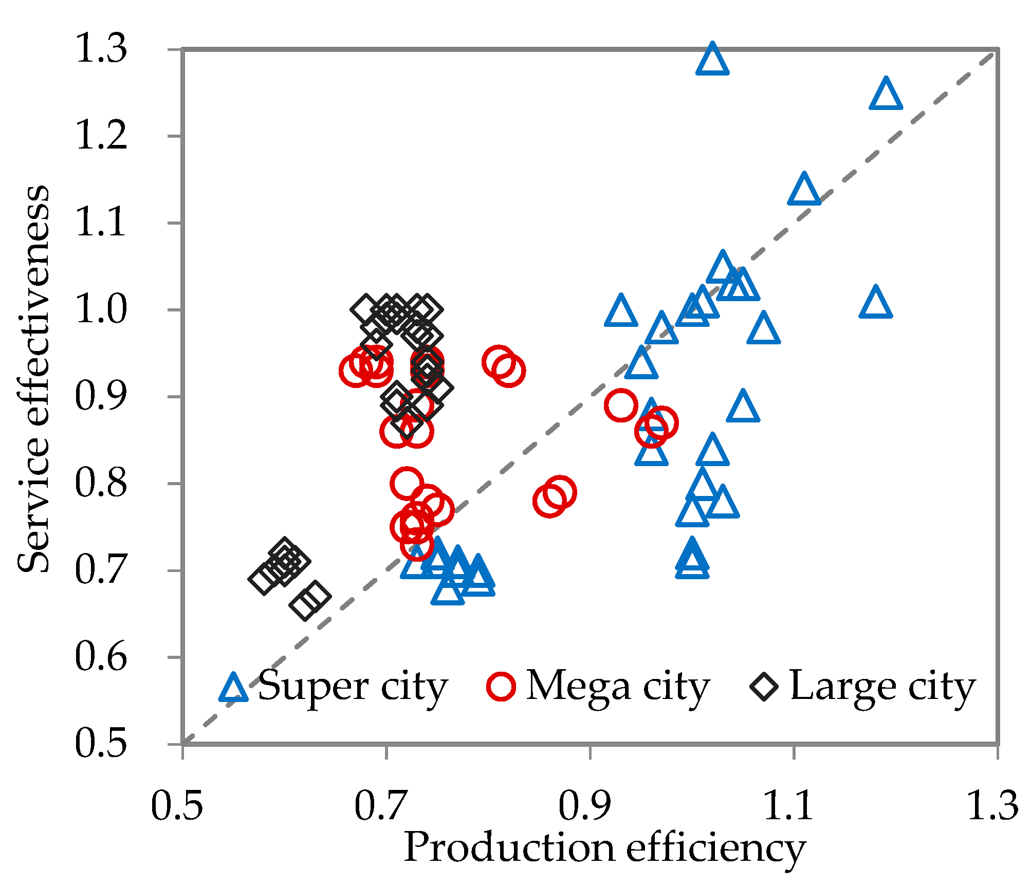
• A city with a large population is more likely to be production-efficient than service-effective, whereas a city with a small population is more likely to be service-effective than production-efficient. Moreover, service effectiveness has a significantly positive correlation with production efficiency. With respect to the overall operational effectiveness, super cities tend to perform better than mega cities, and mega cities tend to perform better than large cities.
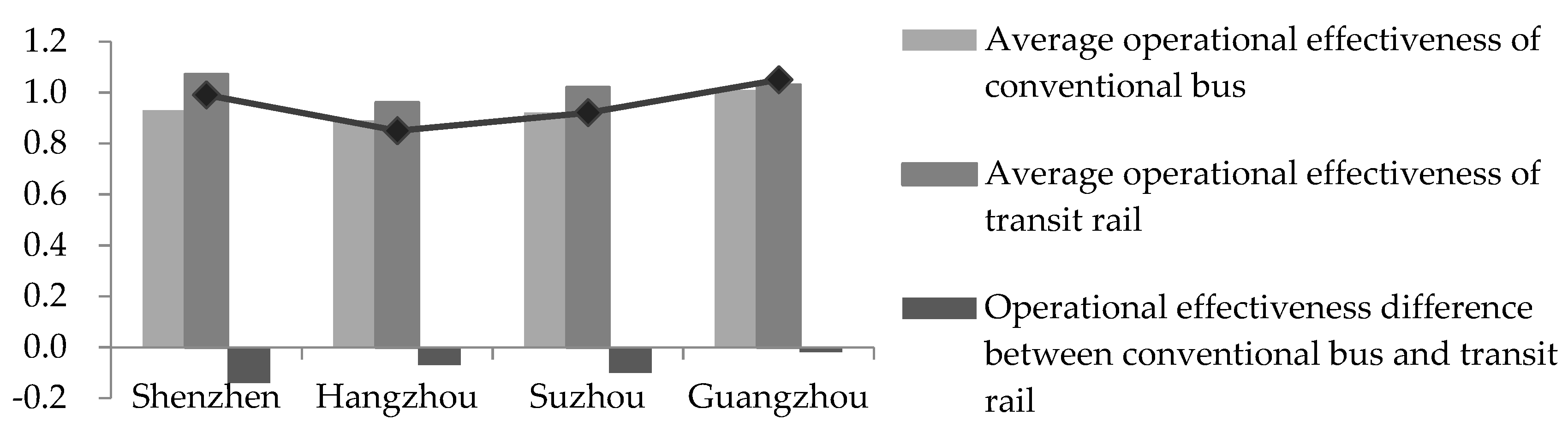
• Transit rail has more operational effectiveness than conventional bus. Moreover, it has the ability to improve a public transit system’s operational effectiveness when developed to a large scale, due to economies of scale.
• By comparing efficiency scores with and without considering exogenous variables, we found that exogenous environment had a marked impact on the performance measurement of the public transit system.
• By projecting inefficient and ineffective transit systems to efficiency and effectiveness, we found that there is a shortage of investment in public transit by both local authority and bus operators in some Chinese cities. Meanwhile, these Chinese cities have a scarcity of transit service and a relatively unsatisfactory impression from passengers.

Several policy implications can be obtained from the results above. First, a city with a large population should pay more attention to service effectiveness, while a city with a small population should be concerned with the production efficiency. Second, with the background of serious air pollution and traffic congestion in China, the large-scale construction of transit rail is a good choice for Chinese large cities. Third, for the inefficient and ineffective transit systems in China, a great deal of support and investment in public transit from local authority and bus operators is still required to increase the supply of public transit services and improve passenger satisfaction.

This paper has some limitations. First, this paper only included specific input and output variables due to problems regarding the availability of high-quality data. For example, regarding input variables, we did not consider bus operators’ fuel consumption, which is a conventional input variable in previous literature [9,26,29]. Second, only several cities have been investigated, and studying more cities may provide more insights. Third, we simply set the consumption process as important as the production process, and did not investigate how the different weighting coefficients would impact the DMUs’ operational effectiveness score. On the basis of these limitations, several future research issues are proposed. First, including more input and output variables may lead to more results. For example, regarding the externality of public transit system, it is reasonable to incorporate CO₂ emissions into the evaluation. Second, the impact of the two weight coefficients (i.e., w1 and w2) on operational effectiveness deserves attention and further study. Finally, in addition to traditional evaluation methods, new methods should be tried and used in the study of public transit performance. For example, predictive markets can be used to forecast public transit demand, and then derive appropriate inputs to achieve effective operation [54]; design thinking can be used to cherish multiple perspectives and rich frameworks of the public transit problem [55].

References

1. Dulebenets, M.A. A novel Memetic Algorithm with a deterministic parameter control for efficient berth scheduling at marine container terminals. Marit. Bus. Rev. 2017, 2, 302–330. [Google Scholar] [CrossRef]
2. Dulebenets, M.A. A comprehensive multi-objective optimization model for the vessel scheduling problem in liner shipping. Int. J. Prod. Econ. 2018, 196, 293–318. [Google Scholar] [CrossRef]
3. Jalalian, M.; Gholami, S.; Ramezanian, R. Analyzing the trade-off between CO2 emissions and passenger service level in the airline industry: Mathematical modeling and constructive heuristic. J. Clean Prod. 2019, 206, 251–266. [Google Scholar] [CrossRef]
4. Wagenaar, J.; Kroon, L.; Fragkos, I. Rolling stock rescheduling in passenger railway transportation using dead-heading trips and adjusted passenger demand. Transp. Res. Pt. B-Methodol. 2017, 101, 140–161. [Google Scholar] [CrossRef]
5. Liu, L.; Chen, R.C. A novel passenger flow prediction model using deep learning methods. Transp. Res. Pt. C-Emerg. Technol. 2017, 84, 74–91. [Google Scholar] [CrossRef]
6. Miller, P.; de Barros, A.G.; Kattan, L.; Wirasinghe, S.C. Analyzing the sustainability performance of public transit. Transport. Res. Part D-Transport. Environ. 2016, 44, 177–198. [Google Scholar] [CrossRef]
7. Venkatesh, A.; Kushwaha, S. Short and long-run cost efficiency in Indian public bus companies using Data Envelopment Analysis. Socio-Econ. Plan. Sci. 2018, 61, 29–36. [Google Scholar] [CrossRef]
8. De Borger, B.; Kerstens, K.; Costa, A. Public transit performance: what does one learn from frontier studies? Transp. Rev. 2002, 22, 1–38. [Google Scholar] [CrossRef]
9. Odeck, J. Congestion, ownership, region of operation, and scale: Their impact on bus operator performance in Norway. Socio-Econ. Plan. Sci. 2006, 40, 52–69. [Google Scholar] [CrossRef]
10. Ottoz, E.; Fornengo, G.; Di Giacomo, M. The impact of ownership on the cost of bus service provision: an example from Italy. Appl. Econ. 2009, 41, 337–349. [Google Scholar] [CrossRef]
11. Hahn, J.S.; Kim, D.K.; Kim, H.C.; Lee, C. Efficiency analysis on bus companies in Seoul city using a network DEA model. KSCE J. Civ. Eng. 2013, 17, 1480–1488. [Google Scholar] [CrossRef]
12. Sheth, C.; Triantis, K.; Teodorović, D. Performance evaluation of bus routes: A provider and passenger perspective. Transp. Res. Pt. e-Logist. Transp. Rev. 2007, 43, 453–478. [Google Scholar] [CrossRef]
13. Kang, C.C.; Khan, H.A.; Feng, C.M.; Wu, C.C. Efficiency evaluation of bus transit firms with and without consideration of environmental air-pollution emissions. Transport. Res. Part D-Transport. Environ. 2017, 50, 505–519. [Google Scholar] [CrossRef]
14. Zhao, Y.; Triantis, K.; Murray-Tuite, P.; Edara, P. Performance measurement of a transportation network with a downtown space reservation system: A network-DEA approach. Transp. Res. Pt. e-Logist. Transp. Rev. 2011, 47, 1140–1159. [Google Scholar] [CrossRef]
15. Yu, M.M.; Fan, C.K. Measuring the performance of multimode bus transit: A mixed structure network DEA model. Transp. Res. Pt. e-Logist. Transp. Rev. 2009, 45, 501–515. [Google Scholar] [CrossRef]
16. Chiu, Y.; Huang, C.; Ma, C.M. Assessment of China transit and economic efficiencies in a modified value-chains DEA model. Eur. J. Oper. Res. 2011, 209, 95–103. [Google Scholar] [CrossRef]
17. Seiford, L.M.; Zhu, J. Modeling undesirable factors in efficiency evaluation. Eur. J. Oper. Res. 2002, 142, 16–20. [Google Scholar] [CrossRef]
18. Chen, C.M.; Du, J.; Huo, J.; Zhu, J. Undesirable factors in integer-valued DEA: Evaluating the operational efficiencies of city bus systems considering safety records. Decis. Support Syst. 2012, 54, 330–335. [Google Scholar] [CrossRef]
19. Chen, X.; Wang, X.; Zhang, H.; Li, J. The diversity and evolution process of bus system performance in chinese cities: An empirical study. Sustainability 2014, 6, 7751–7767. [Google Scholar] [CrossRef]
20. Kassens-Noor, E.; Kotval-K, Z.; Brush, A.; Doshier, K.; Biskey, M. Michigan’s Public Transportation: An Application of Statewide Performance Assessment and Management. Available online: https://www.sciencedirect.com/science/article/pii/S2590198219300132 (accessed on 27 June 2019).
21. Monast, K.; Stanfield, C. An analysis of success plans and performance measures for rural transit systems in North Carolina. Transp. Res. Record. 2019, 2673, 97–105. [Google Scholar] [CrossRef]
22. Roy, W.; Yvrande-Billon, A. Ownership, contractual practices and technical efficiency: The case of urban public transport in France. J. Transp. Econ. Policy 2007, 41, 257–282. Available online: https://www.ingentaconnect.com/content/lse/jtep/2007/00000041/00000002/art00006 (accessed on 27 June 2019).
23. Boitani, A.; Nicolini, M.; Scarpa, C. Do competition and ownership matter? Evidence from local public transport in Europe. Appl. Econ. 2013, 45, 1419–1434. [Google Scholar] [CrossRef]
24. Zhang, C.; Juan, Z.; Xiao, G. Do contractual practices affect technical efficiency? Evidence from public transport operators in China. Transp. Res. Pt. e-Logist. Transp. Rev. 2015, 80, 39–55. [Google Scholar] [CrossRef]
25. Viton, P.A. Technical efficiency in multi-mode bus transit: A production frontier analysis. Transp. Res. Pt. B-Methodol. 1997, 31, 23–39. [Google Scholar] [CrossRef]
26. Boame, A.K. The technical efficiency of Canadian urban transit systems. Transp. Res. Pt. e-Logist. Transp. Rev. 2004, 40, 401–416. [Google Scholar] [CrossRef]
27. Sampaio, B.R.; Neto, O.L.; Sampaio, Y. Efficiency analysis of public transport systems: Lessons for institutional planning. Transp. Res. Pt. A-Policy Pract. 2008, 42, 445–454. [Google Scholar] [CrossRef] [Green Version]
28. Hawas, Y.E.; Khan, M.; Basu, N. Evaluating and enhancing the operational performance of public bus systems using GIS-based data envelopment analysis. J. Publ. Transp. 2012, 15, 19–44. [Google Scholar] [CrossRef]
29. Azadi, M.; Shabani, A.; Khodakarami, M.; Saen, R.F. Planning in feasible region by two-stage target-setting DEA methods: An application in green supply chain management of public transportation service providers. Transp. Res. Pt. e-Logist. Transp. Rev. 2014, 70, 324–338. [Google Scholar] [CrossRef]
30. Gattoufi, S.; Oral, M.; Kumar, A.; Reisman, A. Content analysis of data envelopment analysis literature and its comparison with that of other OR/MS fields. J. Oper. Res. Soc. 2004, 55, 911–935. [Google Scholar] [CrossRef]
31. Farrell, M.J. The measurement of productive efficiency. J. R. Stat. Soc. Ser. A-Gen. 1957, 120, 253–290. [Google Scholar] [CrossRef]
32. Charnes, A.; Cooper, W.W.; Rhodes, E. Measuring the efficiency of decision making units. Eur. J. Oper. Res. 1978, 2, 429–444. [Google Scholar] [CrossRef]
33. Von Hirschhausen, C.; Cullmann, A. A nonparametric efficiency analysis of German public transport companies. Transp. Res. Pt. e-Logist. Transp. Rev. 2010, 46, 436–445. [Google Scholar] [CrossRef]
34. Lao, Y.; Liu, L. Performance evaluation of bus lines with data envelopment analysis and geographic information systems. Comput. Environ. Urban Syst. 2009, 33, 247–255. [Google Scholar] [CrossRef]
35. Karlaftis, M.G. A DEA approach for evaluating the efficiency and effectiveness of urban transit systems. Eur. J. Oper. Res. 2004, 152, 354–364. [Google Scholar] [CrossRef]
36. Tsamboulas, D.A. Assessing performance under regulatory evolution: A European transit system perspective. J. Urban Plan. Dev. 2006, 132, 226–234. [Google Scholar] [CrossRef]
37. Georgiadis, G.; Politis, I.; Papaioannou, P. Measuring and improving the efficiency and effectiveness of bus public transport systems. Res. Transp. Econ. 2014, 48, 84–91. [Google Scholar] [CrossRef]
38. Pina, V.; Torres, L. Analysis of the efficiency of local government services delivery. An application to urban public transport. Transp. Res. Pt. A-Policy Pract. 2001, 35, 929–944. [Google Scholar] [CrossRef]
39. Zhang, C.; Juan, Z.; Luo, Q.; Xiao, G. Performance evaluation of public transit systems using a combined evaluation method. Transp. Policy 2016, 45, 156–167. [Google Scholar] [CrossRef]
40. Karlaftis, M.G.; Tsamboulas, D. Efficiency measurement in public transport: Are findings specification sensitive? Transp. Res. Pt. A-Policy Pract. 2012, 46, 392–402. [Google Scholar] [CrossRef]
41. Caulfield, B.; Bailey, D.; Mullarkey, S. Using data envelopment analysis as a public transport project appraisal tool. Transp. Policy 2013, 29, 74–85. [Google Scholar] [CrossRef] [Green Version]
42. Kain, J.F.; Liu, Z. Secrets of success: assessing the large increases in transit ridership achieved by Houston and San Diego transit providers. Transp. Res. Pt. A-Policy Pract. 1999, 33, 601–624. [Google Scholar] [CrossRef]
43. Taylor, B.D.; Miller, D.; Iseki, H.; Fink, C. Nature and/or nurture? Analyzing the determinants of transit ridership across US urbanized areas. Transp. Res. Pt. A-Policy Pract. 2009, 43, 60–77. [Google Scholar] [CrossRef] [Green Version]
44. Chakraborty, A.; Mishra, S. Land use and transit ridership connections: Implications for state-level planning agencies. Land Use Pol. 2013, 30, 458–469. [Google Scholar] [CrossRef]
45. Banker, R.D.; Morey, R.C. Efficiency analysis for exogenously fixed inputs and outputs. Oper. Res. 1986, 34, 513–521. [Google Scholar] [CrossRef]
46. Färe, R.; Grosskopf, S. Network dea. Socio-econ. Plan. Sci. 2000, 34, 35–49. [Google Scholar] [CrossRef]
47. Andersen, P.; Petersen, N.C. A procedure for ranking efficient units in data envelopment analysis. Manage. Sci. 1993, 39, 1261–1264. [Google Scholar] [CrossRef]
48. Scheel, H. Undesirable outputs in efficiency valuations. Eur. J. Oper. Res. 2001, 132, 400–410. [Google Scholar] [CrossRef]
49. Vencheh, A.H.; Matin, R.K.; Kajani, M.T. Undesirable factors in efficiency measurement. Appl. Math. Comput. 2005, 163, 547–552. [Google Scholar] [CrossRef]
50. Liu, W.; Sharp, J. DEA models via goal programming. In Data Envelopment Analysis in the Service Sector; Westermann, G., Ed.; Deutscher Universitätsverlag: Wiesbaden, Germany, 1999; Volume 5, pp. 79–101. [Google Scholar]
51. Berg, S.A.; Førsund, F.R.; Jansen, E.S. Malmquist indices of productivity growth during the deregulation of Norwegian banking, 1980-89. Scandinavian J. Econ. 1992, 94, S211–S228. [Google Scholar] [CrossRef]
52. Yu, M.M. Assessing the technical efficiency, service effectiveness, and technical effectiveness of the world’s railways through NDEA analysis. Transp. Res. Pt. A-Policy Pract. 2008, 42, 1283–1294. [Google Scholar] [CrossRef]
53. Li, J.; Xu, L.; Yao, D.; Mao, Y. Impacts of symbolic value and passenger satisfaction on bus use. Transport. Res. Part D-Transport. Environ. 2019, 72, 98–113. [Google Scholar] [CrossRef]
54. Czwajda, L.; Kosacka-Olejnik, M.; Kudelska, I.; Kostrzewski, M.; Sethanan, K.; Pitakaso, R. Application of prediction markets phenomenon as decision support instrument in vehicle recycling sector. LogForum 2019, 15, 265–278. [Google Scholar] [CrossRef]
55. Kostrzewski, M. One Design Issue—Many Solutions. Different Perspectives of Design Thinking—Case Study. In Knowledge Management in Organizations. KMO 2018. Communications in Computer and Information Science; Uden, L., Hadzima, B., Ting, I.H., Eds.; Springer: Cham, Switzerland, 2018; Volume 877. [Google Scholar]
Figure 1. The structure of the public transit system.
Sustainability 11 03555 g001
Figure 2. The measurement framework of the public transit system.
Sustainability 11 03555 g002
Figure 3. Service effectiveness versus production efficiency.
Sustainability 11 03555 g003
Figure 4. Operational effectiveness trends over time.
Sustainability 11 03555 g004
Figure 5. Operational effectiveness comparison between conventional bus and transit rail.
Sustainability 11 03555 g005
Figure 6. Production efficiency versus subsidies.
Sustainability 11 03555 g006
Figure 7. Production efficiency versus the length of bus lines.
Sustainability 11 03555 g007
Figure 8. Production efficiency versus employees.
Sustainability 11 03555 g008