Abstract
The identification of geographical distribution of a plant species is crucial for understanding the importance of environmental variables affecting plant habitat. In the present study, the spatial potential distribution of Astragalus fasciculifolius Boiss. as a key specie was mapped using maximum entropy (Maxent) as data mining technique and bivariate statistical model (FR: frequency ratio) in marl soils of southern Zagros, Iran. The A. fasciculifolius locations were identified and recorded by intensive field campaigns. Then, localities points were randomly split into a 70% training dataset and 30% for validation. Two climatic, four topographic, and eight edaphic variables were used to model the A. fasciculifolius distribution and its habitat potential. Maps of environmental variables were generated using Geographic Information System (GIS). Next, the habitat suitability index (HSI) maps were produced and classified by means of Maxent and FR approaches. Finally, the area under the receiver operating characteristic (AUC-ROC) curve was used to compare the performance of maps produced by Maxent and FR models. The interpretation of environmental variables revealed that the climatic and topographic parameters had less impact compared to edaphic variables in habitat distribution of A. fasciculifolius. The results showed that bulk density, nitrogen, acidity (pH), sand, and electrical conductivity (EC) of soil are the most significant variables that affect distribution of A. fasciculifolius. The validation of results showed that AUC values of Maxent and FR models are 0.83 and 0.76, respectively. The habitat suitability map by the better model (Maxent) showed that areas with high and very high suitable classes cover approximately 22% of the study area. Generally, the habitat suitability map produced using Maxent model could provide important information for conservation planning and a reclamation project of the degraded habitat of intended plant species. The distribution of the plants identifies the water, soil, and nutrient resources and affects the fauna distribution, and this is why it is relevant to research and to understand the plant distribution to properly improve the management and to achieve a sustainable management.
1. Introduction
Spatial and temporal distribution of species is affected by the quality and quantity of habitats [1,2]. Species distribution models (SDMs) are generally used to predict the habitat potential and spatial distribution of a species according to the occurrence data and different environmental variables [3,4,5]. These models have been widely used for many different purposes in ecological and conservation studies to evaluate the relationship between species occurrence and environmental variables [6,7,8]. Reliable data collection of species’ spatial distribution could provide important information for conservation planning, reclamation projects of degraded habitats, and prediction of anthropogenic and climatic impacts on habitat potential of a plant species. A variety of statistical and probabilistic models is currently used to determine the spatial distribution of plant species [5,9,10,11,12]. Among the common SDMs used in the recent literature are the statistical models such as generalized linear models (GLMs: [9,13] and generalized additive models (GAMs: [14,15,16]) and also probabilistic models such as Maxent [5,17,18,19] and frequency ratio (FR). Among different species distribution models, Maxent has been proven suitable to predict the habitat potential of plant species based on presence-only occurrence data [5,6,18,20,21]. Although among the mentioned models, the FR algorithm mainly has been used for predicting the natural hazard such as landslide [22,23,24,25], its application in species distribution modeling has not been well documented.
The Maharlou Watershed located in the southern Zagros Mountain is exposed extensively to the deposits from hill slopes with marl soils originated from Gachsaran, Razak, and Sachoun geological formations [26]. Western parts of Maharlou Hill slopes are traditionally used for livestock grazing by nomads and rural communities, as well as agricultural activities, leading to plant diversity loss and accelerated soil erosion. This area is suffering from severe water erosion due to widespread marl soil distribution and has the high potential for severe land degradation process. It has been proven that marl soils are very sensitive to water erosion and mass movement due to human-induced land use changes and agricultural activities. Furthermore, sediments produced from marl soils could increase water pollution and flooding events, decrease reservoir capacity, and lead to soil and plant diversity loss [27]. On the other hand, the positive impact of vegetation on water erosion control has been widely studied in the literature reviews [28,29]. Hence, in arid and semiarid regions, identification and restoration of native plant communities that exist or appear in the erosion process prior to desertification are very important for landscape restoration planning [30,31,32]. Astragalus fasciculifolius (Fabaceae) is a 0.5–1.5 m high perennial thorny shrub mainly found in hill slopes of southern Zagros in the Fars, Bushehr, Khuzestan, and Hormozgan Provinces. A. fasciculifolius shows high ecological values in terms of soil conservation, livestock feeding, carbon sequestration potential, and medicinal properties [33,34,35,36].
In the present study, the FR bivariate statistical model and Maxent data mining technique were used to predict and map the distribution of A. fasciculifolius in marl soils of Maharlou Watershed, Fars Province, Iran.
So, the aims of the current research are:
- (1)
- to quantify the relationship between A. fasciculifolius and the selected environmental variables;
- (2)
- to develop the habitat suitability index (HSI) and identify the additional and potential localities of A. fasciculifolius and targeting the marl soil conservation activities, as well as vegetation restoration planning; and,
- (3)
- to compare between FR and Maxent models for predicting the potential distribution of A. fasciculifolius in the study area.
2. Materials and Methods
Figure 1 indicates the methodology flowchart of the current study. This figure shows the process involved in the conditioning environmental variables preparation, models application, and their validation.
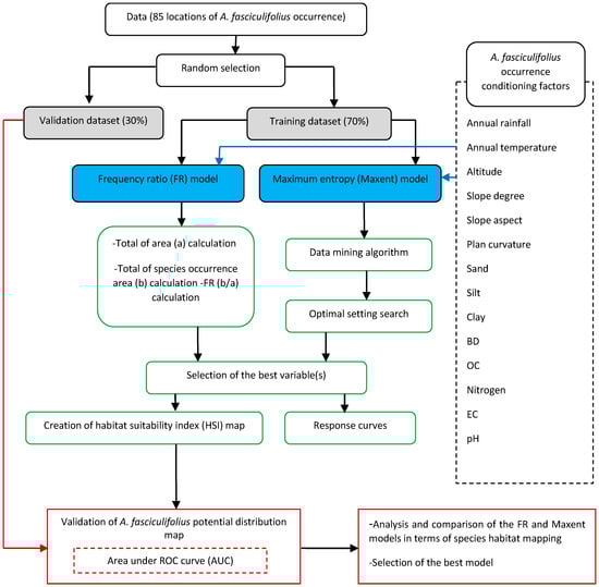
Figure 1.
Flowchart of the used methodology in the current study. AUC-ROC: area under the receiver operating characteristic curve.
2.1. Study Area
The study area, western parts of Maharlou Watershed, is located in Fars Province, southern Iran (29°31′–29°54′N and 52°12′–52°41′E), with an area of 265 square km inside the Zagros Mountains (Figure 2). It receives 510 mm annual rainfall with average annual temperature of 17 °C [37]. The minimum and maximum elevation ranges from 1500 to 2700 m above sea level, respectively. Vegetation of the study area is dominated by A. fasciculifolius Boiss, along with plant species of Ebenus stellata Boiss., Convolvulus leiocalycinus Boiss., Gundelia tournefortii L., Phlomis elliptica Benth., and Stipa barbata Desf. Considering the widespread marl soils in the western parts of Maharlou Watershed and using a geology map, the boundaries of marl formations as key indicators for soil conservation were extracted and used as a base map for data sampling and future analyses (Figure 2).
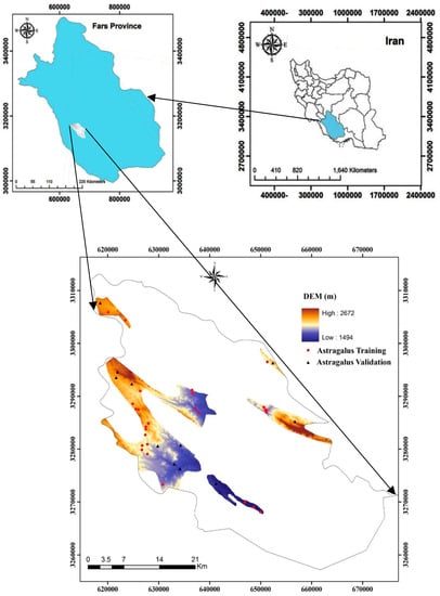
Figure 2.
Location map of the study area in Iran, Fars Province, and distribution of sampling points.
2.2. Data Used
2.2.1. Species Description
Astragalus is one of the largest and most widespread genera of Fabaceae family, including 3280 species distributed all over the world. In general, 844 species of this genus are grown wildly in Iran, of which 620 species (73.4%) are endemic [38,39,40,41]. A. fasciculifolius is a perennial woody plant growing wild in southern parts of the Zagros Mountains (Figure 3). It has thorny branches and deep taproots. A. fasciculifolius is a xerophyte plant that is well adapted to marl soils of the southern Zagros and plays an important role in the conservation of marl soils; besides, it has some industrial and medicinal uses for the local people of the southern Zagros, Iran [33,42,43].
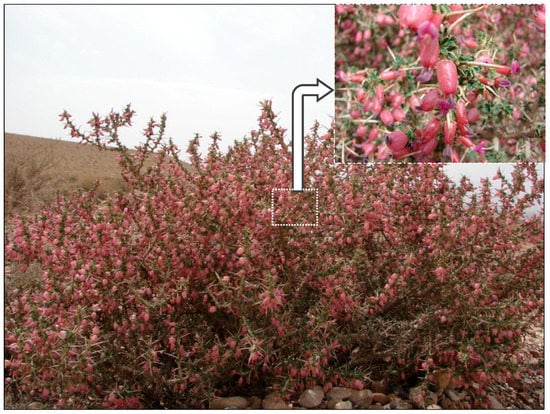
Figure 3.
View and detail of Astragalus fasciculifolius Boiss. from the Dehshikh study area, Iran.
2.2.2. Species Occurrence Data
A total of 85 occurrence records of A. fasciculifolius were collected during field surveys in 2015 and 2016, from April to September, in hill slope parts of western Maharlou Watershed. The longitude and latitude of species localities were recorded using a handheld Global Positioning System (GPS) receiver (Garmin Map 62s) and the geographical distribution database of A. fasciculifolius was compiled (Figure 2).
2.3. Geo-Environmental Variables
2.3.1. Climatic Data
Climatic data were obtained from 18 stations in the study area (http://www.irimo.ir). Mean annual precipitation and temperature maps were prepared using inverse distance weight (IDW) and kriging interpolation approaches (Figure 3a,b). It has to be noted that these variables are very important in environmental modeling (Table 1) and are frequently used in species distribution models [11,44].

Table 1.
Environmental predictors used for modelling the habitat suitability of A. fasciculifolius.
2.3.2. Topographic Data
Digital Elevation Model (DEM) with a pixel size of 20 m × 20 m (http://www.ncc.org.ir) was used to generate altitude, slope angle, aspect, and plan curvature layers using Arc GIS 10.1 (ESRI, Redlands, CA, USA). The altitude thematic layer was categorized into 4 classes (Figure 4c) and the slope angle map was classified into 5 classes (Figure 4d). The slope aspect and plan curvature maps (Table 1) were calculated using DEM and then generated and categorized into 5 and 3 classes, respectively (Figure 3e,f).
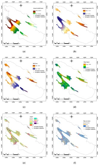
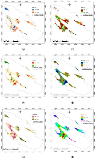
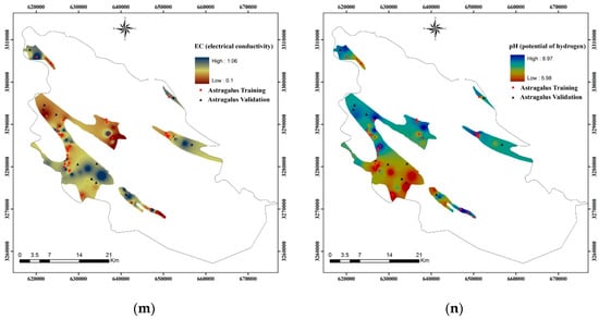
Figure 4.
Maps of geo-environmental conditioning variables: (a) annual rain; (b) annual temperature; (c) altitude; (d) slope degree; (e) slope aspect; (f) plan curvature; (g) sand; (h) silt; (i) clay; (j) bulk density (BD); (k) organic carbon (OC); (l) nitrogen; (m) electrical conductivity (EC) and (n) pH.
2.3.3. Soil Data Mapping
Based on A. fasciculifolius spatial distribution, soil samples were taken in 0–30 cm depth of plant habitat. In total, 85 soil samples were taken. Then, the number of the most important physical and chemical soil parameters including sand, silt, clay, organic matter, electrical conductivity (EC), nitrogen, organic carbon (OC), bulk density (BD), and acidity (pH) was determined in the laboratory. The air-dried soil samples were sieved through a screen with 2 mm mesh size and prepared for the analysis. Soil texture and pH were determined using hydrometer method [45,46] and an electric pH meter [47], respectively. Also, soil EC was determined from a 1:1 soil–water suspension using an EC meter [48]. Soil organic carbon (OC) and nitrogen were measured using the Walkley–Black [49] and Kjeldahl methods [47]. Soil bulk density was identified using a core sampler of 8 cm diameter [49]. The soil data resulting from laboratory analysis was mapped (Table 1) and interpolated through kriging techniques (Figure 3g,n). At first, the spatial variability of each soil sample was determined and semi-variograms were calculated. Then, the most appropriate model was fitted and the cross-validation approach was used to ensure the appropriation of the selected model.
2.4. Models Description
2.4.1. Frequency Ratio (FR) Model
The frequency ratio (FR) model supposes that the species occurrence will happen at similar conditions as if it occurs now. Moreover, the FR model is based on the assumption that the larger ratio means the stronger relationship between spatial species occurrence and the given geo-environmental variables [23,24,50]. In fact, the frequency ratio is a bivariate statistical model that could be expressed as the frequency ratio of each variable [51,52]. This approach is based on the relationship between species spatial distribution and all geo-environmental factors contributing to species occurrence in the habitats [24,53]. This approach is a simple and reliable model used in many fields of research [23,53,54,55,56]. This model can be expressed by the following equation [24,25]:
where FR is the frequency ratio of class i of parameter j, Npix is the number of pixels with species occurrence within class i of parameter variable x, is the number of pixels with parameter variable xj, and n is the number of classes in the parameter variable xi in the study area [24,25].
The FR value of 1 indicates the area in which species occurrence and FR value less than 1 shows a lower probability of species occurrence. Therefore, the higher ratio value indicates the stronger the relationship between species occurrence and the given variable’s class attribute, while the lower the value means the lower probability of the species occurrence in the study area [23,25].
2.4.2. Maximum Entropy (Maxent) Model
Maxent model is a machine learning/data mining program that evaluates the distribution probability of a species in relation to environmental factors [12,17,57]. This model has a general-purpose approach to estimate the probability distribution of a species, proven to work well in practical studies [7]. Maxent uses presence-only data and makes spatial predictions from now occurrence data to predict the distribution of a species. Indeed, Maxent model estimates the spatial distribution probability of a species that is closest to uniform and still subjected to environmental variable constraints. Also, it attempts to predict the habitat suitability for a species [5,17,20].
Maxent could support categorical and continuous predictor data varying from 0 as the lowest to 1 as the highest suitability. If we suppose a random variable j that has n different potential results as x1, x2, …, xn, then the occurrence probabilities are p1, p2, …, pn, respectively. The equation of Maxent is as follows [2,23,58]:
where a is the area of category and b represents the area of species occurrence percentages within the given category, (Pij) is the probability density, Hj and Hjmax are entropy values, Ij represents the information coefficient, and Wj represents the resultant weight value for the parameter as a whole (Equations (2)–(7)).
The practical application of the Maxent model in habitat suitability for plant species has been proven in several investigations [2,10,11,12,18,59,60]. The Maxent program used in this study was obtained from http://biodiversityinformatics.amnh.org/open_source/maxent/. It can be downloaded free of charge for scientific research activities. The detailed description of this model and practical manual is presented by Phillips et al. (2006) [17], Elith et al. (2011) [20] and Phillips et al. (2017) [61]. In this research, 70% and 30% of data were assigned for model training and validation, respectively [62].
2.5. Models Validation
The FR and Maxent results were validated using the threshold-independent area under the curve (AUC) of receiver operating characteristics (ROC) [63]. This approach is one of the most widely used statistics for model evaluation. The AUC value ranges from 0.5 to 1.0, where value <0.5 describes no fit to the data; in contrast, 1.0 value indicates perfect model performance, and values >0.9 imply a very high performance. In general, the higher AUC value shows the higher performance of the model [60,63,64].
3. Results and Discussion
3.1. FR Model
The results of the FR model for all the data layers are shown in Figure 5. To visualize the results, the results of the species occurrence were classified into categorical occurrence classes in accordance with the natural breaks method [65].
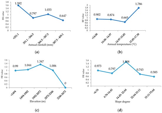
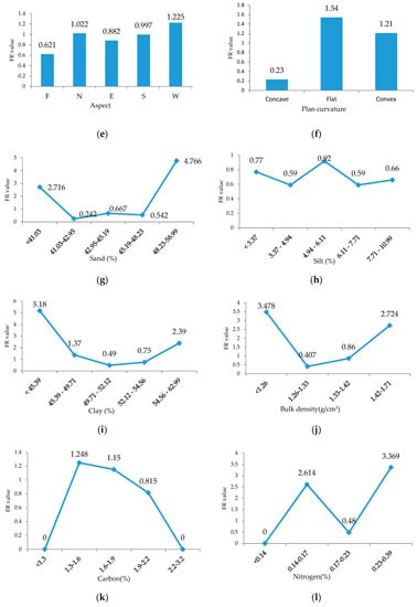
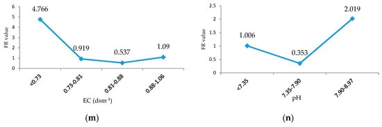
Figure 5.
Response curve for geo-environmental conditioning variables: (a) annual rain, (b) annual temperature, (c) altitude, (d) slope degree, (e) slope aspect, (f) plan curvature, (g) sand, (h) silt, (i) clay, (j) BD, (k) OC, (l) nitrogen, (m) EC, and (n) pH.
In the FR model, each factor’s rating was assigned as the relationship between A. fasciculifolius occurrence and given environmental variables. As shown in Figure 5, the annual rain less than 351.8 mm indicates the highest FR value of 1.59. In the case of annual temperature, it is seen that the value of FR (1.78) is greater for temperatures in the range of 15.85–17.40. The effect of slope aspect on the occurrence of a plant species had been noticed [66,67,68]. For the slope angle, it is shown that 14–22° and <6° have 35.29 and 29.41% of probability to species occurrence with FR value of 1.51 and 0.97, respectively. The species frequency in the elevation class of 1902–2072 m is higher (1.35) than the other classes, followed by 1725–1902 m classes with an FR value of 1.04. It is seen that west (1.23) and north (1.02) slope facing have greater probability to A. fasciculifolius and the flat areas showed the lowest FR value of 0.621. For plan curvature, the flat indicates the greater value of FR (1.53) followed by convex curvature (1.21). In the case of soil texture, as shown in Figure 5, the 48.23–58.99% sand class with FR value of 4.77 and clay class of <45.39% (FR value of 5.18) have the highest FR value than other classes. Previous research showed a well-developed deep root system in perennial woody shrubs such as A. fasciculifolius in arid and semiarid environments [69,70]. The soil texture of study habitat mainly composed of sandy–clay soils permits deep root percolation in soil layers and uptake water from lower soil layers in dry seasons [71]. In the case of bulk density, the class <1.26 grcm–3 had a considerably greater FR value (3.48) and the species occurrence was larger than other classes. With regard to organic carbon (OC), the FR value of 1.3–1.6% indicated the greater value (1.25), followed by the 1.6–1.9% class with a value of 1.15. Considerable research has shown that woody perennial shrubs produce more aboveground litters and, accordingly, improve soil organic carbon and fertility [72,73,74]. For nitrogen (N), the results showed that the range between 0.23 and 0.39%, with FR value of 3.37, seem to have a higher impact on A. fasciculifolius occurrence. The higher level of nitrogen in habitat soil of A. fasciculifolius indicates the positive impact of legume plants such as Astragalus genus on the nitrogen fixation process, which have been well studied [75]. The frequency ratio between A. fasciculifolius occurrence and EC indicated that the higher FR values (Figure 5) are related to the class of <0.73 dsm–1 (4.77), suggesting the negative impact of salinity on habitat of A. fasciculifolius. Several research studies have shown the occurrence of Astragalus on non-saline soils in the mountainous parts of Iran [76,77,78]. According to the frequency ratio model results, A. fasciculifolius occurrence density is highest at the acidity (pH) ranging from 7.90 to 8.99, with FR value of 2.02. Due to widespread calcareous geology formation in the study area, the studied species prefers neutral to alkaline soils [79].
Finally, the habitat suitability index (HSI) was calculated by summation of each variable ratio value, as shown in Equation (8) (Lee et al. 2015):
where HSI is the habitat suitability index and FR is the frequency ratio value of each variable. The HSI represents the relative habitat potential to species occurrence. So, the greater FR value means the higher suitability of habitat for species occurrence. The resulting map of HSI is shown in Figure 6. The HSI value of the final FR map ranges from 7.81 to 32.78. This value represents the relative habitat potential index to A. fasciculifolius occurrence. The index values were classified into four classes (low, moderate, high, and very high) using the natural break (NB) method (Figure 6). The classified areas in the low and moderate classes are 55.71 and 25.85%, respectively. On the other hand, the areas in the high and very-high HSI classes are 14.21 and 4.23%, respectively (Figure 6). Generally, the high and very-high A. fasciculifolius occurrence areas included around 18.44% of the total of the study area.
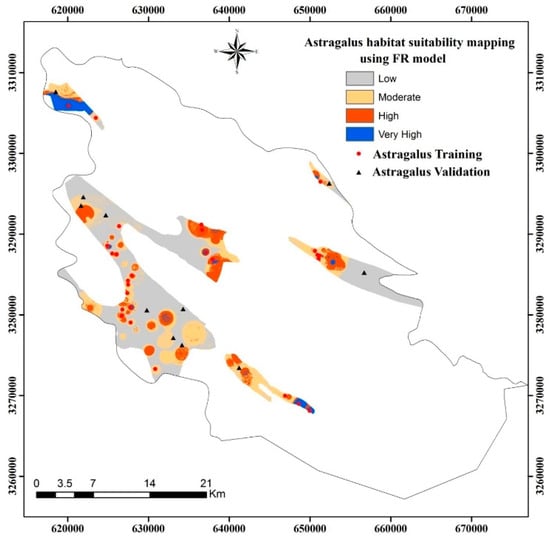
Figure 6.
Habitat suitability distribution of A. fasciculifolius based on the FR model.
3.2. Maxent Model
The Maxent model for A. fasciculifolius performed very well with an AUC value of 82.6%. Table 2 and Figure 7 indicate the achieved results for given geo-environmental variables. Based on Maxent model assumption, if a pixel in the study area has equal condition of the rating data, it would assign the higher value. Meanwhile, the pixels with different environmental conditions are assigned with lower values [10].
Table 2.
Maxent values of all variable classes.
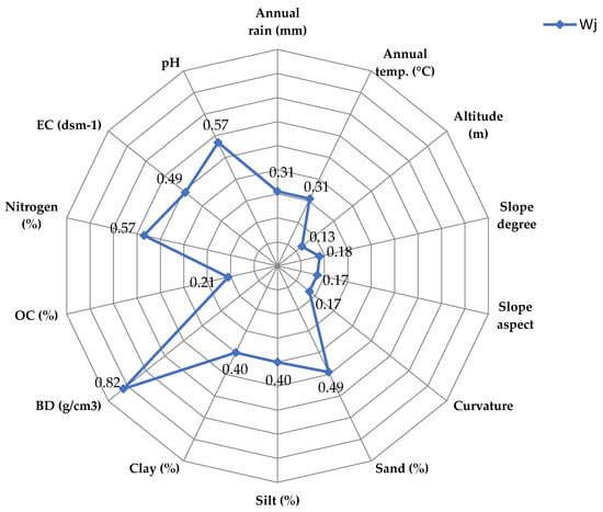
Figure 7.
Final weights of conditioning variables generated by Maxent model.
Based on the results generated by the Maxent model (Table 2), BD, nitrogen, and pH with probability value of 0.82, 0.57, and 0.57 were the most useful variables with the highest impact on the habitat suitability, followed by sand percent (0.49), EC (0.49), clay percent (0.40), and silt percent (0.39), while other variables had less impact on the habitat suitability index of the study area.
Consequently, suitable habitats for A. fasciculifolius were predicted in parts with bulk density of <1.26 grcm–3, soil nitrogen content of >0.23%, pH with value of >7.90, and clay content of <45.39% in the study area (Table 2, Figure 7).The habitat suitability for A. fasciculifolius increased with decreasing electrical conductivity; however, it decreased slowly with increasing of soil clay content (Figure 7). These results indicate that A. fasciculifolius prefers western/northern slopes with sandy–clay, non-saline soils. These results are in line with Ghanbarian and Tayebi Khorrami’s (2005) [80] understanding of A. Fasciculifolius as a shrubby legume plant with a high adaptation level to the hill slopes of the Zagros Mountains, in southern Iran. The suitable annual mean temperature higher than 15.85 °C and annual rain less than 332.5 mm indicated that A. fasciculifolius favors warmer and drier locations. [33,36,38] reported that A. fasciculifolius is normally found in the arid and semiarid regions of the Fars, Bushehr, Khuzestan, and Hormozgan Provinces in southern Iran.
Overall, the contribution of soil factors including BD, nitrogen, pH, and clay, except organic carbon, were relatively strong in A. fasciculifolius occurrence, but the impact of the climate variables such as annual rain and annual temperature was moderate. Meanwhile, the impact of topographic factors such as elevation, slope degree, slope aspect, and plan curvature were relatively very weak in occurrence of A. fasciculifolius.
The final HSI map by Maxent model was developed using Arc GIS 10.1 software based on the Equation (9):
HIS = (annual rainfall × 0.313) + (annual temperature × 0.309) + (altitude × 0.126) + (slope degree × 0.181) + (slope aspect × 0.170) + (Plan curvature × 0.173) + (sand × 0.499) + (silt × 0.395) + (clay × 0.401) + (bulk density × 0.822)+ (organic carbon × 0.210) + (nitrogen × 0.568) + (electrical conductivity × 0.489) + (pH × 0.568)
Consequently, a HSI map was obtained and classified into four classes of low, moderate, high, and very high based on a given training data set, as mentioned for the FR model (Figure 8). The HSI values range from 2.79 to 14.07. Based on the HSI map generated by Maxent model, very-high and high suitable habitats covered 7.41% and 14.50% of the total study area, respectively. Moderate suitable locations consisted of 26.26%, followed by low (51.82%) suitable areas.
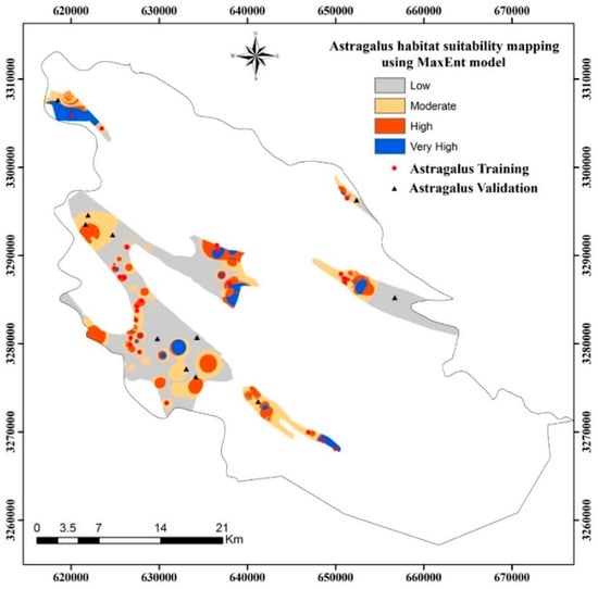
Figure 8.
Habitat suitability distribution of A. fasciculifolius based on Maxent model.
3.3. Validation of the HSI Maps and Comparison between FR and Maxent Models
In the current study, the validation of habitat suitability maps was conducted using ROC curve [23]. Based on literature review, the ROC curve represents the quality of deterministic and probabilistic detection and could be a useful approach to rely on the prediction models of a plant species [11]. The ROC curves (PRC-prediction rate curve) of FR and Maxent models were illustrated in Figure 9. The area under the ROC curve (AUC) was used to evaluate and compare both FR and Maxent model performance.
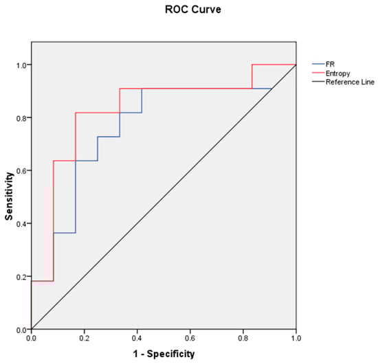
Figure 9.
ROC curve of sensitivity vs. specificity of A. fasciculifolius habitat for Maxent and FR models.
The habitat suitability results indicated an AUC value of 0.826 and 0.758 for the Maxent and FR model, respectively (Table 3).
Table 3.
The area under the curve (AUC) value for Maxent and FR models.
The results of both models provided satisfactory output for habitat suitability prediction. Although, the Maxent model showed a better result compared to FR approach. In previous research, Hosseini et al. (2013) [10], Khanum et al. (2013) [11], and Sahragard and Chahouki (2015) [19] showed that the Maxent model could be a satisfactory tool with high accuracy potential for predicting the suitable habitats of plant species. On the other hand, some researchers showed reasonable application of the FR model for potential distribution modelling of natural hazards such as fire and landslide and also groundwater potential mapping [23,24,59,81]. In general, the Maxent and FR models are good estimators of A. fasciculifolius habitat in the study area. Although, the Maxent model showed slightly better results for habitat suitability mapping. On the other hand, data clustering has been suggested as new research in unsupervised learning algorithm that could be applied in different fields of ecology including, plant distribution and habitat suitability studies. This is a suggestion for future research efforts in species distribution modeling [82,83,84]. In general, there are different data mining techniques that are applied in geosciences and environmental engineering in cases of landslides, forest fires, land subsidence, flood, and gully erosion, including random forest-RF [85,86,87,88,89,90], support vector machine-SVM [90,91,92], multivariate adaptive spline regression-MARS [93,94], and boosted regression tree-BRT [95]. Even in a case on groundwater modeling, Rahmati et al. 2016 [69] considered a comparison between two data mining techniques, including random forest and Maxent models. Their results showed that accuracy of two models was 86.5 and 91%. So, the findings indicated that Maxent is better than random forest in the modelling process. So, it is important to mention that the Maxent data mining model as a traditional approach in comparison to other recent data mining techniques could present reasonable results; thus, in the current study, we tried to use the Maxent model for species distribution modelling and its results comprised to a bivariate statistical model entitled the FR as it is known as a basic model for considering the relationship between independent and dependent variables in literature reviews. The HSI maps could be a useful tool for conservation agencies and land managers for conservation and reclamation of degraded habitats of A. fasciculifolius.
3.4. Soil as a Key Factor
Our research has shown that soil is the key factor to determine the plant distribution. This is a key finding as it demonstrates that soil conservation should be applied where there is a need to preserve the plant cover. Soil is a key issue to achieve sustainable development, as the United Nations shows in their goals for Sustainable Development [96]. Moreover, in arid and semiarid countries, there is a need to find a proper management to fight against land degradation and it is a challenge to achieve the Land Degradation Neutrality [97]. There is a need to understand the soil and plant interaction to develop restoration programs. Research on the interaction of soils and plants shows how the fate of the ecosystems is dependent on soil erosion [98]. More and more, soil erosion is found to be a key link between the plant and the soil world as plants control the soil losses, but the soil quality and the soil erosion determine the plant distribution [99]. This is mainly due to the role that soil erosion exerts on seed redistribution and then on soil erosion [100]. The connectivity of the flows and sediments, and then seeds, is a relevant concept to be used in future research on plant distribution, as the flows determines the fate of the soil particles and then the seeds [101].
4. Conclusions
In the current study, a habitat suitability model was developed using FR and Maxent models to evaluate and predict the current and potential areas suitable for A. fasciculifolius in marl soils of the Zagros Mountains, southern Iran. Among the 14 variables selected for the model development, A. fasciculifolius habitat was mainly influenced by soil parameters including bulk density, nitrogen content, electrical conductivity, acidity, and clay percent. The climate and topographic variables showed relative weak impact in determination of habitat suitability of A. fasciculifolius. The Maxent model has reasonable and relative accurate outputs as well as FR for predicting the habitat suitability of A. fasciculifolius in our study area. The habitat suitability maps produced using FR and Maxent approach were classified into four classes including very high, high, moderate, and low. The verification of the results showed that both FR and Maxent models are reasonable for habitat suitability prediction. Although, the result of the Maxent model was better than the FR approach. Therefore, the areas predicted and mapped as the favorite places for A. fasciculifolius could be considered for current and future conservation planning. It could be suggested that more detailed soil maps and more climatic layers could also be used in habitat suitability mapping of the studied plant species to achieve more precise suitability map. Our findings can be applied in different ways such as of the protection of the sensitive habitats of A. fasciculifolius and reclamation of the degraded marl soil vegetation in the study area. More attention should be paid in the future to investigate environmental variables that could influence the A. fasciculifolius due to climate change and human-induced activities.
Author Contributions
For research articles with several authors, a short paragraph specifying their individual contributions must be provided. The following statements should be used “conceptualization, G.G. and H.R.P.; Methodology, H.R.P, R.S; Software, M.M.; Validation, M.M., G.G. and H.R.P; Formal analysis, G.G., M.M; investigation, G.G., M.M; Writing—original draft preparation, M.M., G.G; Writing—review and editing, H.R.P., A.C.; Project administration, G.G., H.R.P.; Funding acquisition, A.C.
Funding
This research was funded by Shiraz University, grant number No.94GCU3M153031.
Conflicts of Interest
The authors declare no conflict of interest.
References
- Purves, D.W.; Dushoff, J. Directed seed dispersal and meta-population response to habitat loss and disturbance: Application to Eichhornia paniculata. J. Ecol. 2005, 93, 658–669. [Google Scholar] [CrossRef]
- Yi, Y.J.; Cheng, X.; Yang, Z.F.; Zhang, S.H. Maxent modeling for predicting the potential distribution of endangered medicinal plant (H. riparia Lour) in Yunnan, China. Ecol. Eng. 2016, 92, 260–269. [Google Scholar] [CrossRef]
- Thorn, J.S.; Nijman, V.; Smith, D.; Nekaris, K.A.I. Ecological niche modelling as a technique for assessing threats and setting conservation priorities for Asian slow lorises (Primates: Nycticebus). Divers. Distrib. 2009, 15, 289–298. [Google Scholar] [CrossRef]
- Wilson, C.D.; Roberts, D.; Reid, N. Applying species distribution modelling to identify areas of high conservation value for endangered species: A case study using Margaritifera margaritifera (L.). Biol. Conserv. 2011, 144, 821–829. [Google Scholar] [CrossRef]
- Qin, A.; Liu, B.; Guo, Q.; Bussmann, R.W.; Ma, F.; Jian, Z.; Xu, G.; Pei, S. Maxent modeling for predicting impacts of climate change on the potential distribution of Thuja sutchuenensis Franch., an extremely endangered conifer from southwestern China. Glob. Ecol. Conserv. 2017, 10, 139–146. [Google Scholar] [CrossRef]
- Pearson, R.G.; Raxworthy, C.J.; Nakamura, M.; Townsend, P.A. Predicting species distributions from small numbers of occurrence records: A test case using cryptic geckos in Madagascar. J. Biogeogr. 2007, 34, 102–117. [Google Scholar] [CrossRef]
- Elith, J.H.; Graham, C.P.; Anderson, R.; Dudík, M.; Ferrier, S.; Guisan, A.J.; Hijmans, R.; Huettmann, F.R.; Leathwick, J.; Lehmann, A.; et al. Novel methods improve prediction of species’ distributions from occurrence data. Ecography 2006, 29, 129–151. [Google Scholar] [CrossRef]
- Elith, J.; Leathwick, J.R. Species distribution models: Ecological explanation and prediction across space and time. Annu. Rev. Ecol. Evol. Syst. 2009, 40, 677–697. [Google Scholar] [CrossRef]
- Guisan, A.; Zimmermann, N.E. Predictive habitat distribution models in ecology. Ecol. Model. 2000, 135, 147–186. [Google Scholar] [CrossRef]
- Hosseini, S.Z.; Kappas, M.; Chahouki, M.Z.; Gerold, G.; Erasmi, S.; Emam, A.R. Modelling potential habitats for Artemisia sieberi and Artemisia aucheri in Poshtkouh area, central Iran using the maximum entropy model and geostatistics. Ecol. Inform. 2013, 18, 61–68. [Google Scholar] [CrossRef]
- Khanum, R.; Mumtaz, A.S.; Kumar, S. Predicting impacts of climate change on medicinal asclepiads of Pakistan using Maxent modeling. Acta Oecol. 2013, 49, 23–31. [Google Scholar] [CrossRef]
- Yang, X.Q.; Kushwaha, S.P.S.; Saran, S.; Xu, J.; Roy, P.S. Maxent modeling for predicting the potential distribution of medicinal plant, Justicia adhatoda L. in Lesser Himalayan foothills. Ecol. Eng. 2013, 51, 83–87. [Google Scholar] [CrossRef]
- Bolker, B.M.; Brooks, M.E.; Clark, C.J.; Geange, S.W.; Poulsen, J.R.; Stevens, M.H.H.; White, J.S.S. Generalized linear mixed models: A practical guide for ecology and evolution. Trends Ecol. Evol. 2009, 24, 127–135. [Google Scholar] [CrossRef] [PubMed]
- Lehmann, A. GIS modeling of submerged macrophyte distribution using Generalized Additive Models. Plant Ecol. 1998, 139, 113–124. [Google Scholar] [CrossRef]
- Austin, M. Species distribution models and ecological theory: A critical assessment and some possible new approaches. Ecol. Indic. 2007, 200, 1–19. [Google Scholar] [CrossRef]
- Cassini, M.H. Ecological principles of species distribution models: The habitat matching rule. J Biogeogr. 2011, 38, 2057–2065. [Google Scholar] [CrossRef]
- Phillips, S.J.; Anderson, R.P.; Schapire, R.E. Maximum entropy modeling of species geographic distributions. Ecol. Model. 2006, 190, 231–259. [Google Scholar] [CrossRef]
- Gastón, A.; García-Viñas, J.I. Modelling species distributions with penalised logistic regressions: A comparison with maximum entropy models. Ecol. Model. 2011, 222, 2037–2041. [Google Scholar] [CrossRef]
- Sahragard, H.P.; Chahouki, M.Z. An evaluation of predictive habitat models performance of plant species in Hozesoltan rangelands of Qom Province. Ecol Modell. 2015, 309, 64–71. [Google Scholar] [CrossRef]
- Elith, J.; Phillips, S.J.; Hastie, T.; Dudík, M.; Chee, Y.E.; Yates, C.J. A statistical explanation of MaxEnt for ecologists. Divers. Distrib. 2011, 17, 43–57. [Google Scholar] [CrossRef]
- Garcia, K.; Lasco, R.; Ines, A.; Lyon, B.; Pulhin, F. Predicting geographic distribution and habitat suitability due to climate change of selected threatened forest tree species in the Philippines. Appl Geogr. 2013, 44, 12–22. [Google Scholar] [CrossRef]
- Demir, G.; Aytekin, M.; Akgün, A.; Ikizler, S.B.; Tatar, O. A comparison of landslide susceptibility mapping of the eastern part of the North Anatolian Fault Zone (Turkey) by likelihood-frequency ratio and analytic hierarchy process methods. Nat. Hazards 2013, 65, 1481–1506. [Google Scholar] [CrossRef]
- Jaafari, A.; Najafi, A.; Pourghasemi, H.R.; Rezaeian, J.; Sattarian, A. GIS-based frequency ratio and index of entropy models for landslide susceptibility assessment in the Caspian forest, Northern Iran. Int. J. Environ. Sci. Technol. 2014, 11, 909–926. [Google Scholar] [CrossRef]
- Youssef, A.M.; Al-Kathery, M.; Pradhan, B. Landslide susceptibility mapping at Al-Hasher area, Jizan (Saudi Arabia) using GIS-based frequency ratio and index of entropy models. Geosci. J. 2015, 19, 113–134. [Google Scholar] [CrossRef]
- Wang, Q.; Li, W.; Yan, S.; Wu, Y.; Pei, Y. GIS based frequency ratio and index of entropy models to landslide susceptibility mapping (Daguan, China). Environ. Earth Sci. 2016, 75. [Google Scholar] [CrossRef]
- GSI (Geological Survey of Iran). Geological Map of Shiraz, 1:250000; National Iranian Oil Company: Tehran, Iran, 1979. [Google Scholar]
- Nadal-Romero, E.; Petrlic, K.; Verachtert, E.; Bochet, E.; Poesen, J. Effects of slope angle and aspect on plant cover and species richness in a humid Mediterranean badland. Earth Surf. Process. Landf. 2014, 39, 1705–1716. [Google Scholar] [CrossRef]
- Gyssels, G.; Poesen, J.; Bochet, E.; Li, Y. Impact of plant roots on the resistance of soils to erosion by water: A review. Prog. Phys. Geogr. 2005, 29, 189–217. [Google Scholar] [CrossRef]
- Bochet, E.; García-Fayos, P.; Poesen, J. Topographic thresholds for plant colonization on semi-arid eroded slopes. Earth. Surf. Process. Landf. 2009, 34, 1758–1771. [Google Scholar] [CrossRef]
- García-Fayos, P.; García-Ventoso, B.; Cerdà, A. Limitations to plant establishment on eroded slopes in southeastern Spain. J. Veg. Sci. 2000, 11, 77–86. [Google Scholar] [CrossRef]
- Guerrero-Campo, J.; Palacio, S.; Montserrat-Martí, G. Plant traits enabling survival in Mediterranean badlands in northeastern Spain suffering from soil erosion. J. Veg. Sci. 2008, 19, 457–464. [Google Scholar] [CrossRef]
- Varavipour, M.; Asadi, T.; Arzjani, Z. Reletionship between the physico-chemical properties and different types of erosion on Marl soils south of Tehran, Iran. Asian J. Chem. 2010, 22, 5201–5208. [Google Scholar]
- Mozaffarian, V. Trees and Shrubs of Iran; Moaser Farhang Publications: Tehran, Iran, 2004. [Google Scholar]
- Shao, B.M.; Xu, W.; Dai, H.; Tu, P.; Li, Z.; Gao, X.M. A study on the immune receptors for polysaccharides from the roots of Astragalus membranaceus, a Chinese medicinal herb. Biochem. Biophys. Res. Commun. 2004, 320, 1103–1111. [Google Scholar] [CrossRef] [PubMed]
- Mosaddegh, M.; Naghibi, F.; Moazzeni, H.; Pirani, A.; Esmaeili, S. Ethnobotanical survey of herbal remedies traditionally used in Kohghiluyehva Boyer Ahmad province of Iran. J. Ethnopharmacol. 2012, 141, 80–95. [Google Scholar] [CrossRef] [PubMed]
- Shahid, M.; Rao, N.K. New records for the two Fabaceae species from the United Arab Emirates. J. New Biol. Rep. 2015, 4, 207–210. [Google Scholar]
- IRIMO. Climate Data-Base. Available online: http://www.weather.ir/English/ (accessed on 16 August 2017).
- Maassoumi, A.A. Astragalus in the Old World; Research Institute of Forests and Rangelands: Tehran, Iran, 1998. [Google Scholar]
- Rechinger, K.H. Flora Iranica, Vol. 175. Papilionaceae IV, Astragalus II; Akademische Verlagsgesellschaft: Salzburg, Austria, 1999. [Google Scholar]
- Frodin, D.G. History and concepts of big plant genera. Taxon 2004, 53, 753–776. [Google Scholar] [CrossRef]
- Podlech, D.; Zarre, S.; Ekici, M.; Maassoumi, A.A.; Sytin, A. A Taxonomic Revision of the Genus Astragalus L. (Leguminosae) in the Old World; Annalen des Naturhistorischen Museums in Wien. Serie B fürBotanik und Zoologie; Naturhistorisches Museum Wien: Wien, Austria, 2014. [Google Scholar]
- Mozaffarian, V. Flora of Khuzestan, Khuzestan Province; Animal Affairs and Natural Resources Research Center Publications: Tehran, Iran, 1999. [Google Scholar]
- Niknam, V.; Lisar, Y.S. Chemical composition of Astragalus: Carbohydrates and mucilage content. Pak. J. Bot. 2004, 36, 381–388. [Google Scholar]
- Sanchez, A.C.; Osborne, P.E.; Haq, N. Climate change and the African baobab (Adansoniadigitata L.): The need for better conservation strategies. Afr. J. Ecol. 2011, 49, 234–245. [Google Scholar] [CrossRef]
- Bouyoucos, G.J. Hydrometer method improved for making particle size analyses of soils. Agron. J. 1962, 54, 464–465. [Google Scholar] [CrossRef]
- Gee, G.W.; Bauder, J.W. Particle-size analysis. In Methods of Soil Analysis: Part 1—Physical and Mineralogical Methods; American Society of Agronomy, Inc.; Soil Science Society of America, Inc.: Madison, WI, USA, 1986. [Google Scholar]
- Bremmer, J.M.; Mulvaney, C.S. Regular Kjeldahl method. In Methods of Soil Analysis Part 2; American Society of Agronomy, Inc.; Soil Science Society of America, Inc.: Madison, WI, USA, 1982. [Google Scholar]
- Carter, M.R. Soil Sampling and Methods of Analysis; CRC Press: Boca Raton, FL, USA, 1993. [Google Scholar]
- Nosetto, M.D.; Jobbagy, E.G.; Paruelo, J.M. Carbon sequestration in semi-arid rangelands: Comparison of Pinus ponderosa plantations and grazing exclusion in NW Patagonia. J. Arid Environ. 2006, 67, 142–156. [Google Scholar] [CrossRef]
- Yalcin, A.; Reis, S.; Aydinoglu, A.C.; Yomralioglu, T. A GIS-based comparative study of frequency ratio, analytical hierarchy process, bivariate statistics and logistics regression methods for landslide susceptibility mapping in Trabzon, NE Turkey. Catena 2011, 85, 274–287. [Google Scholar] [CrossRef]
- Bonham-Carter, G.E.; Cox, S.J.D. Geographic information systems for geoscientists: Modelling with GIS. Econ. Geol. 1995, 90, 1352–1353. [Google Scholar]
- Lee, M.J.; Song, W.; Lee, S. Habitat mapping of the leopard cat (Prionailurus bengalensis) in South Korea using GIS. Sustainability 2015, 7, 4668–4688. [Google Scholar] [CrossRef]
- Lee, S.; Pradhan, B. Landslide hazard mapping at Selangor, Malaysia using frequency ratio and logistic regression models. Landslides 2007, 4, 33–41. [Google Scholar] [CrossRef]
- Pradhan, B.; Lee, S. Delineation of landslide hazard areas on Penang Island, Malaysia, by using frequency ratio, logistic regression, and artificial neural network models. Environ. Earth. Sci. 2010, 60, 1037–1054. [Google Scholar] [CrossRef]
- Mohammady, M.; Pourghasemi, H.R.; Pradhan, B. Landslide susceptibility mapping at Golestan Province, Iran: A comparison between frequency ratio, Dempster-Shafer, and weights-of-evidence models. J. Asian Earth Sci. 2012, 61, 221–236. [Google Scholar] [CrossRef]
- Pourghasemi, H.R.; Mohammady, M.; Pradhan, B. Landslide susceptibility mapping using index of entropy and conditional probability models in GIS: Safarood Basin, Iran. Catena 2012, 97, 71–84. [Google Scholar] [CrossRef]
- Phillips, S.J.; Dudík, M.; Schapire, R.E. A maximum entropy approach to species distribution modeling. In Proceedings of the Twenty-First International Conference on Machine Learning, Banff, AB, Canada, 4–8 July 2004; p. 83. [Google Scholar]
- Constantin, M.; Bednarik, M.; Jurchescu, M.C.; Vlaicu, M. Landslide susceptibility assessment using the bivariate statistical analysis and the index of entropy in the Sibiciu Basin (Romania). Environ. Earth. Sci. 2011, 63, 397–406. [Google Scholar] [CrossRef]
- White, E.P.; Thibault, K.M.; Xiao, X. Characterizing species abundance distributions across taxa and ecosystems using a simple maximum entropy model. Ecology 2012, 93, 1772–1778. [Google Scholar] [CrossRef] [PubMed]
- Yuan, H.S.; Wei, Y.L.; Wang, X.G. Maxent modeling for predicting the potential distribution of Sanghuang, an important group of medicinal fungi in China. Fungal Ecol. 2015, 17, 140–145. [Google Scholar] [CrossRef]
- Phillips, S.J.; Dudík, M.; Schapire, R.E. Maxent Software for Modeling Species Niches and Distributions Version 3.4.0. Available online: http://biodiversityinformatics.amnh.org/open_source/maxent/ (accessed on 17 April 2018).
- Rahmati, O.; Pourghasemi, H.R.; Melesse, A.M. Application of GIS-based data driven random forest and maximum entropy models for groundwater potential mapping: A case study at Mehran Region, Iran. Catena 2016, 137, 360–372. [Google Scholar] [CrossRef]
- Fielding, A.H.; Bell, J.F. A review of methods for the assessment of prediction errors in conservation presence/absence models. Environ. Conserv. 1997, 24, 38–49. [Google Scholar] [CrossRef]
- Pearce, J.; Ferrier, S. Evaluating the predictive performance of habitat models developed using logistic regression. Ecol. Model. 2000, 133, 225–245. [Google Scholar] [CrossRef]
- Ayalew, L.; Yamagishi, H. The application of GIS-based logistic regression for landslide susceptibility mapping in the Kakuda-Yahiko Mountains, Central Japan. Geomorphology 2005, 65, 15–31. [Google Scholar] [CrossRef]
- Badano, E.I.; Cavieres, L.A.; Molina-Montenegro, M.A.; Quiroz, C.L. Slope aspect influences plant association patterns in the Mediterranean matorral of central Chile. J. Arid Environ. 2005, 62, 93–108. [Google Scholar] [CrossRef]
- Bennie, J.; Huntley, B.; Wiltshire, A.; Hill, M.O.; Baxter, R. Slope, aspect and climate: Spatially explicit and implicit models of topographic microclimate in chalk grassland. Ecol. Model. 2008, 216, 47–59. [Google Scholar] [CrossRef]
- Gong, X.; Brueck, H.; Giese, K.M.; Zhang, L.; Sattelmacher, B.; Lin, S. Slope aspect has effects on productivity and species composition of hilly grassland in the Xilin River Basin, Inner Mongolia, China. J. Arid Environ. 2008, 72, 483–493. [Google Scholar] [CrossRef]
- Jobbágy, E.G.; Jackson, R.B. The vertical distribution of soil organic carbon and its relation to climate and vegetation. Ecol. Appl. 2000, 10, 423–436. [Google Scholar] [CrossRef]
- Schenk, H.J.; Jackson, R.B. Rooting depths, lateral root spreads and below-ground/above-ground allometries of plants in water-limited ecosystems. J. Ecol. 2002, 90, 480–494. [Google Scholar] [CrossRef]
- Cammeraat, E.; van Beek, R.; Kooijman, A. Vegetation succession and its consequences for slope stability in SE Spain. Plant Soil 2005, 278, 135–147. [Google Scholar] [CrossRef]
- Wezel, A.; Rajot, J.L.; Herbrig, C. Influence of shrubs on soil characteristics and their function in Sahelian agro-ecosystems in semi-arid Niger. J. Arid Environ. 2000, 44, 383–398. [Google Scholar] [CrossRef]
- Pei, S.; Fu, H.; Wan, C. Changes in soil properties and vegetation following exclosure and grazing in degraded Alxa desert steppe of Inner Mongolia, China. Agric. Ecosyst. Environ. 2008, 124, 33–39. [Google Scholar] [CrossRef]
- Wang, S.; Zhao, X.; Qu, H.; Zuo, X.; Lian, J.; Tang, X.; Powers, R. Effects of shrub litter addition on dune soil microbial community in Horqin sandy land, northern China. Arid Land Res. Manag. 2011, 25, 203–216. [Google Scholar] [CrossRef]
- Masson-Boivin, C.; Giraud, E.; Perret, X.; Batut, J. Establishing nitrogen-fixing symbiosis with legumes: How many rhizobium recipes? Trends Microbiol. 2009, 17, 458–466. [Google Scholar] [CrossRef] [PubMed]
- Ranjbar, M.; Karamian, R. Some remarks on the genus Astragalus sect. Incani in Iran. Bot. J. Linn. Soc. 2003, 143, 443–447. [Google Scholar] [CrossRef][Green Version]
- Ranjbar, M. Astragalus sect. Trachycercis (Fabaceae) in Iran. Nord. J. Bot. 2009, 27, 328–335. [Google Scholar] [CrossRef]
- Ahmadi, A.; Shahmoradi, A.A.; Zarekia, S.; Ahmadi, E.; Nateghi, S. Autecological study of Astragalus effusus in rangelands of west Azarbaijan province, Iran. Iran J. Range Desert Res. 2013, 20, 172–181. [Google Scholar]
- Khormali, F.; Abtahi, A. Origin and distribution of clay minerals in calcareous arid and semi-arid soils of Fars Province, southern Iran. Clay Miner. 2003, 38, 511–527. [Google Scholar] [CrossRef]
- Ghanbarian, G.; Tayebi Khorrami, M. Ecological Regions of Iran: Vegetation Types of Jahrom Area; Technical Publication; Research Institute of Forest and Rangelands: Tehran, Iran, 2005. [Google Scholar]
- Manap, M.A.; Nampak, H.; Pradhan, B.; Lee, S.; Sulaiman, W.N.A.; Ramli, M.F. Application of probabilistic-based frequency ratio model in groundwater potential mapping using remote sensing data and GIS. Arab. J. Geosci. 2014, 7, 711–724. [Google Scholar] [CrossRef]
- Soloviev, A.A.; Zharkikh, J.I.; Krasnoperov, R.I.; Nikolov, B.P.; Agayan, S.M. GIS-oriented solutions for advanced clustering analysis of geoscience data using ArcGIS platform. Russ. J. Earth Sci. 2016, 16. [Google Scholar] [CrossRef]
- Wong, K.C.; Peng, C.; Li, Y.; Chan, T.M. Herd clustering: A synergistic data clustering approach using collective intelligence. Appl. Soft Comput. 2014, 23, 61–75. [Google Scholar] [CrossRef]
- Barbosa, S.M.; Gouveia, S.; Scotto, M.G.; Alonso, A.M. Wavelet-based clustering of sea level records. Math. Geosci. 2016, 48, 149–162. [Google Scholar] [CrossRef]
- Jaafari, A.; Pourghasemi, H.R. Factors influencing regional scale wildfire probability in Iran: An application of random forests and support vector machines. In Spatial Modeling in GIS and R for Earth Science and Environmental; Pourghasemi, H.R., Gokceoglu, C., Eds.; Elsevier: Amsterdam, The Netherlands, 2019; pp. 607–619. [Google Scholar]
- Pourghasemi, H.R.; Mohseni Saravi, M. Land-Subsidence Spatial Modeling using Random Forest Data Mining Technique. In Spatial Modeling in GIS and R for Earth Science and Environmental; Pourghasemi, H.R., Gokceoglu, C., Eds.; Elsevier: Amsterdam, The Netherlands, 2019; pp. 147–159. [Google Scholar]
- Youssef, A.M.; Pourghasemi, H.R.; Pourtaghi, Z.; Al-Katheeri, M.M. Landslide susceptibility mapping using random forest, boosted regression tree, classification and regression tree, and general linear models and comparison of their performance at Wadi Tayyah Basin, Asir region, Saudi Arabia. Landslides 2016, 13, 839–856. [Google Scholar] [CrossRef]
- Naghibi, S.A.; Pourghasemi, H.R.; Dixon, B. Groundwater spring potential using boosted regression tree, classification and regression tree, and random forest machine learning models in Iran. Environ. Monit. Assess. 2016, 188, 44. [Google Scholar] [CrossRef] [PubMed]
- Hong, H.; Pourghasemi, H.R.; Pourtaghi, Z.S. Landslide susceptibility assessment in Lianhua County (China): A comparison between a random forest data mining technique and bivariate and multivariate statistical. Geomorphology 2016, 259, 105–118. [Google Scholar] [CrossRef]
- Chen, W.; Pourghasemi, H.R.; Kornejady, A.; Zhang, N. Landslide spatial modeling: Introducing new ensembles of ANN, MaxEnt, and SVM machine learning techniques. Geoderma 2017, 305, 314–327. [Google Scholar] [CrossRef]
- Abdollahi, S.; Pourghasemi, H.R.; Ghanbarian, G.A.; Safaeian, R. Prioritization of effective factors in the occurrence of land subsidence and its susceptibility mapping using SVM model and their different kernel functions. Bull. Eng. Geol. Environ. 2018, 1–18. [Google Scholar] [CrossRef]
- Ljubomir, G.; Pourghasemi, H.R.; Drobnjak, S.; Bai, S. Testing a new ensemble model based on SVM and Random forest in forest fire susceptibility assessment and its mapping in Serbian National Park Tara. Forests 2019, 10, 408. [Google Scholar]
- Pourghasemi, H.R.; Rossi, M. Landslide susceptibility modeling in a landslide prone area in Mazandarn Province, North of Iran: A comparison between GLM, GAM, MARS, and M-AHP methods. Theor. Appl. Climatol. 2017, 130, 609–633. [Google Scholar] [CrossRef]
- Zabihi, M.; Pourghasemi, H.R.; Pourtaghi, Z.S.; Behzadfar, M. GIS-based multivariate adaptive regression spline and random forest models for groundwater potential mapping in Iran. Environ. Earth. Sci. 2016, 75, 665. [Google Scholar] [CrossRef]
- Zabihi, M.; Pourghasemi, H.R.; Motevalli, A.; Zakeri, M.A. Gully Erosion Modeling Using GIS-Based Data Mining Techniques in Northern Iran: A Comparison Between Boosted Regression Tree and Multivariate Adaptive Regression Spline. Natural hazards GIS-based spatial modeling using data mining techniques. In Natural Hazards GIS-Based Spatial Modeling Using Data Mining Techniques; Pourghasemi, H.R., Rossi, M., Eds.; Springer: Cham, Switzerland, 2019; pp. 1–26. [Google Scholar]
- Keesstra, S.D.; Bouma, J.; Wallinga, J.; Tittonell, P.; Smith, P.; Cerdà, A.; Montanarella, L.; Quinton, J.N.; Pachepsky, Y.; van der Putten, W.H.; et al. The significance of soils and soil science towards realization of the United Nations Sustainable Development Goals. Soil 2016, 2, 111–128. [Google Scholar] [CrossRef]
- Keesstra, S.; Mol, G.; de Leeuw, J.; Okx, J.; de Cleen, M.; Visser, S. Soil-related sustainable development goals: Four concepts to make land degradation neutrality and restoration work. Land 2018, 7, 133. [Google Scholar] [CrossRef]
- Berendse, F.; van Ruijven, J.; Jongejans, E.; Keesstra, S. Loss of plant species diversity reduces soil erosion resistance. Ecosystems 2015, 18, 881–888. [Google Scholar] [CrossRef]
- Cerdà, A. The effect of patchy distribution of Stipa tenacissima L. on runoff and erosion. J. Arid Environ. 1997, 36, 37–51. [Google Scholar] [CrossRef]
- García-Fayos, P.; Bochet, E.; Cerdà, A. Seed removal susceptibility through soil erosion shapes vegetation composition. Plant Soil 2010, 334, 289–297. [Google Scholar] [CrossRef]
- Keesstra, S.; Nunes, J.P.; Saco, P.; Parsons, T.; Poeppl, R.; Masselink, R.; Cerdà, A. The way forward: Can connectivity be useful to design better measuring and modelling schemes for water and sediment dynamics? Sci. Total Environ. 2018, 644, 1557–1572. [Google Scholar] [CrossRef]
© 2019 by the authors. Licensee MDPI, Basel, Switzerland. This article is an open access article distributed under the terms and conditions of the Creative Commons Attribution (CC BY) license (http://creativecommons.org/licenses/by/4.0/).